Udding [3] and was extended by Dill [4]; we provide structural constructions and ..... We would like to thank David Dill, Jerry Burch, Daniel Weise, Peter Beerel, ...
Automatic Verification of Timed Circuits Tomas G. Rokicki? and Chris J. Myers?? Stanford University Stanford, CA 94305
Abstract. This paper presents a new formalism and a new algorithm for verifying timed circuits. The formalism, called orbital nets, allows hierarchical verification based on a behavioral semantics of timed trace theory. We present improvements to a geometric timing algorithm that take advantage of concurrency by using partial orders to reduce the time and space requirements of verification. This algorithm has been fully automated and incorporated into a design system for timed circuits, and experimental results demonstrate that this verification algorithm is practical for realistic examples.
1 Introduction Timing considerations are critical in circuit design. In the design of timed circuits, timing information is taken into account resulting in simpler circuits than their speedindependent counterparts in which gate delays are assumed to be unbounded [1]. Timing information must also be considered for designs with a mixed synchronous/asynchronous environment. Finally, even in speed-independent circuit design, timing must be considered when verifying the isochronic fork and atomic gate assumptions [2] once the circuit is laid out and delay parameters can be estimated. Timed circuit verification is difficult both because circuit elements and circuit communication must be accurately modeled, and because timing considerations introduce another exponential factor of complexity. To address these problems, we start with a formalism of synchronized finite-state agents, modeled by labeled safe Petri nets, with structural constructions for receptiveness and failures. To this formalism, we add timing such that structural constructions on nets correspond to behavioral operations from timed trace theory. Finally, we introduce a new verification algorithm that allows efficient exploration of the entire timed state space. Untimed trace theory for circuit verification originated with Rem, Snepscheut, and Udding [3] and was extended by Dill [4]; we provide structural constructions and syntactic shorthands for labeled safe Petri nets that correspond to the behavioral semantics operations. Burch [5] extended trace theory semantics to timed circuits; we extend this work with an operational formalism that allows timing in the specification, and thus hierarchical timed verification. ? Supported by a John and Fannie Hertz Fellowship and an ARCS fellowship. Currently at
Hewlett-Packard Laboratories, Palo Alto, CA 94306.
?? Supported by an NSF Fellowship, ONR Grant no. N00014-89-J-3036, and research grants
from the Center for Integrated Systems, Stanford University and the Semiconductor Research Corporation, Contract no. 93-DJ-205.
[2,inf]c
[4,10]b
a+
b-
ab+
d+
b-,c+ a+,c-
b+,c-
c-
d+
c+
c-
d-
c+ d-
a-,c+ [4,10]b
(a)
(b)
[2,inf]c
(c)
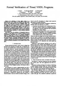
Fig. 1. (a) A fast NAND gate with inputs a and b and output c, (b) a delay buffer with input c and output d, and (c) with timing requirements annotated b for behavior and c for constraint.
Dill [6], Lewis [7], and Berthomieu and Diaz [8] originated geometric state space exploration, and it has become an active area of research [9, 10, 11]. We improve these techniques for systems with concurrency using partial orders and apply them to circuit verification. Recent work by Yoneda et. al. [12] also presented efficient verification through partial order considerations. Our work differs in that our formalism includes notions of specification, circuit composition, and receptiveness which enable us to perform efficient verification on nontrivial timed circuit examples; to our knowledge, neither timed automata nor Time Petri nets have been used in this fashion. Finally, our verification procedure computes a preorder conformance relation, allowing hierarchical verification.
2
Orbital Nets
In this section, we describe orbital nets and show how timed trace theory can be used as a behavioral semantics for verification. For brevity, we assume the reader is familiar with Petri nets [13] and with trace theory [4]. Orbital nets are based on labeled safe Petri nets extended with automatic net constructions and syntactic shorthands for composition and receptiveness [15]. The net constructions allow us to retain relatively straightforward operational semantics, while the syntactic shorthands allow us to compose the nets without an exponential blowup in net size. Orbital nets also allow us to easily mix behavior and environmental requirements even at the gate model level. For a large class of speed-independent and delay-insensitive designs, any hazard is potentially fatal [14], so simple delay models that are easy to integrate into gate models suffice. With the more complex delay models required for modeling real-time circuit delay, such integration is no longer easy or straightforward. Labeling each transition in an orbital net with a (possibly empty) set of actions remedies this difficulty by separating the modeling of the function of a gate from its delay behavior. As an example, the net corresponding to an infinitely fast NAND gate is given in figure 1(a).
2.1 Behavioral Semantics For behavioral semantics, we adopt trace theory as defined by Dill [4]. Using a framework of Petri nets with synchronization and receptiveness, implementing verification of trace structure conformance is straightforward. Determining whether an implementation conforms to a specification is reduced to determining if any of a specific set of failure transitions can be enabled. Dill’s trace theory is based on sequences of actions, but our nets allow transitions to be labeled with sets of actions. A trace theory based on sequences of sets of actions yields a conformance relation that distinguishes, for instance, interleaved and concurrent actions. In addition, composing a net that uses interleaving on a pair of actions with another net that has those same actions labeling one transition may lead to an unintended deadlock. We do not attempt to resolve the complexities that arise in use of such a trace theory. Instead, we define conservative structural conditions on the use of labels consisting of sets of actions that allow us to use Dill’s trace theory. For instance, we cannot perform a trace theory analysis of the fast NAND gate given above, but when we compose that model with the simple buffer given in figure 1(b) and hide the internal wire, the resulting net is conformation equivalent to the model Dill presents in [4]. 2.2 Timing Requirements Timing is associated with an orbital net place as a timing requirement consisting of a lower bound, an upper bound, and a type (min; max; type). The lower bound is a nonnegative integer and the upper bound is an integer greater than or equal to the lower bound, or 1. Since real values can be expressed as rationals within any required accuracy, restricting the bounds of timing requirements to be integers does not decrease the expressiveness of orbital nets. Since there are only a finite number of timing parameters, if any are rational, we can multiply all of them by the least common denominator. There are two types of timing requirements: constraint and behavior. If any transitions in the postset of a place are labeled with an input action, then the timing requirement is of type constraint, otherwise it is of type behavior. Informally, the distinction between behavior and constraint timing requirements follows precisely the difference between input and output actions. The net for the untimed buffer shown in figure 1(b) only describes the successful traces, which are all the prefixes of (c?; d?; c+; d+)� . The receptiveness construction adds failure traces caused by an input event that deviates from this pattern. The net generates only successful output sequences, but it accepts all input sequences, dividing them into success and failure traces. Consider now the buffer pictured in figure 1(c), in which our buffer model has been extended with timing requirements. The behavioral place labeled [4; 10] indicates that an output will occur between 4 and 10 time units after the preceding input occurs; no traces violating this requirement will be generated by the net. The constraint places labeled [2; 1] indicate that, while the net will accept any timing between an output event and the succeeding input event, only those that have a delay of 2 time units or more are successful traces. The delay model just described is an extremely simple delay model that suffices for many types of circuits. More complex delay models can and have been constructed,
modeling more accurately the behavior of a gate under hazard conditions; for these, separation of gate models into combinational function and delay behavior is essential. Each transition can have at most one behavior place in its preset. The intent is that each behavior place represents a single nondeterministic choice of delay that cannot be affected by external state or other behavior places. Since behavior places precede outputs and each wire can be an output for only a single model, circuit composition satisfies this naturally if each component model does. In general, this restriction does not limit expressiveness; other timing semantics can be simulated with appropriate net constructions. 2.3
Timed Operational Semantics
Each token that resides in a constraint or behavior place has a time-valued age parameter which advances with time and describes how long the token has resided in the place. The function max-advance on a marking is defined as the minimum value of (max ? age) for all marked behavior places, or 1 if there are no marked behavior places. This upper limit on time advancement maintains the ages of all behavior place tokens below the maximum allowed by their range. Time is advanced by increasing the ages of all tokens in timed places by precisely the same amount. A transition is untimed-enabled if all places in its preset have tokens. A transition is timed-enabled if it is untimed-enabled and if any input place with a behavior timing requirement has a token with age � min. Transition firings are assumed to be instantaneous; any number of transitions can fire without time advancing. Before firing a transition, the constraint places in the entire net are checked, and if any contains a token with age > max, this firing is marked as a failure. The tokens in the places in the preset of the fired transition are removed. The ages of the tokens removed from constraint places are checked, and if age < min, this firing is marked as a failure. Tokens are then put into the places in the postset of the fired transition, and all tokens put into timed places are assigned an age of zero. After the firing of a transition, every marked behavior place must have a transition in its postset that is untimed-enabled in the new state; if this condition is not satisfied, the firing is a failure. This requirement ensures that every token in a behavior place is consumable in all states in which its timing conditions are met, and thus the age at which the token is consumed cannot be controlled by external state. With these semantics, untimed constructions for receptiveness and synchronization apply unchanged to the timed case. In addition, the trace theory operation of mirroring is also preserved, allowing hierarchical verification. To discuss the verification procedure, we define a timed firing sequence to be a sequence of pairs of transition firings and time values. For simplicity, we shall assume the time value represents a non-negative duration since the last transition firing. Executing a timed firing sequence � on an orbital net results in the timed state fire(�). The set of legal firing sequences is defined recursively as follows. The empty sequence is a legal firing sequence. For a legal firing sequence � and for every value of � such that � � max-advance(fire(�)), then �; (�; � ) is a legal firing sequence, where � represents an ‘empty’ firing. In addition, if transition t is timed-enabled, then �; (t; 0) is also a legal firing sequence.
10
0
10
0
10
0
10
0
10
(a)
(b)
0
0
10
(c)
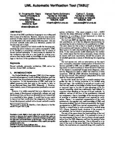
Fig. 2. (a) Discrete, (b) unit cube, and (c) geometric timed state space representations.
We define an untimed state to be an orbital net marking ignoring the ages of the tokens. The function untime returns an untimed firing sequence from a timed firing sequence by stripping the timing and removing any � firings. The reachable state space is the range of the function fire over the legal firing sequences.
3 Discrete and Unit-Cube Time Verification The basic idea behind finite-state verification is that, if the reachable state space is finite or has a finite representation, only a finite subset of the firing sequences needs to be considered to compute the set of reachable states. In our timing semantics, the ages of tokens can be real values, so the state space is infinite. In order to perform finite-state verification, we must either restrict the set of values that these ages can attain, or group the timed states into a finite number of equivalence classes. Discrete time verification uses the first approach, while Alur’s unit-cube technique uses the second. (Infinite upper bounds are easily handled; we shall omit the details here [15].) The first approach is justified by the proof that considering only integer event times gives a full characterization of the continuous time behavior of an orbital net [15]. This proof is similar to one given by Henzinger, et. al. in [16] for timed transition systems. With this result and the operational semantics given above, finite-state verification techniques can now be employed. Indeed, this discrete time approach was taken by Burch for verifying timed circuits [5]. Let us assume the number of distinct untimed states in an orbital net is jS j. If the maximum value of any timing requirement is k, and there are at most n timed tokens in any state (this value is trivially bounded by the size of our safe net), the size of the state space represented by discrete points, as in figure 2(a), is jS j (k + 1)n. If the equivalence between discrete and continuous time does not hold for a particular formalism, it is still possible to perform finite-state real-time verification, using Alur’s unit-cube technique [17]. He considers equivalence classes of timed states with the same integral clock values and a particular linear ordering of the fractional values of the clocks. For the two-dimensional case, the equivalence classes are pictured in figure 2(b); every point, line segment, and interior triangle is an equivalence class. The worst-case size of the state space for his method is asymptotically
jS j lnn!2
�
k ln 2
�n
41=k;
which is worse than the discrete time method by more than n! [15]. Both of these techniques, however, are of little more than theoretical interest, because the size of the state space increases exponentially with the maximum value of the timing requirements. In general, during verification, every possible integer firing time must be considered for every transition from each state. For a circuit with timing values accurate to two significant digits, with up to six independent concurrent pending events, the state space is easily in excess of 1012 states—well beyond the capabilities of most finite-state verification techniques. Our experimental results indicate that the number of discrete states can be astronomical.
4
Geometric Timing Verification
In this section, we discuss a known time verification technique, geometric timing, that usually performs well in practice, even though the worst-case performance is much worse than either the discrete or the unit cube approaches [6, 7, 8, 9, 10, 11]. 4.1
Geometric Regions
Rather than consider at each step a single discrete timed state, or a minimum equivalence class of timed states, the geometric timing method considers a large number of timed states in parallel. Specifically, convex geometric regions of timed states represented by upper and lower bounds on specific clock values and on the differences between pairs of specific clock values are used as the representation of the timed state space. Two sample regions are given in figure 2(c). The set of such constraints is usually represented by a matrix a, where the constraints on clocks fc1 : : :cn g are of the form ci ? cj � aji. A fictitious clock c0 that is always exactly zero is introduced so that upper and lower limits on a particular clock can be represented in the same form [6]. For any convex region that can be represented by such a matrix, there are many matrices that represent the same convex region. The process of canonicalization [6] can be performed to yield a matrix such that every constraint is maximally tight; if the constraint system represented by the matrix has any solutions, then there is precisely one canonicalized matrix representing that region. This canonicalization can be performed with Floyd’s algorithm, which runs in time O(n3 ). In general, since only incremental changes are made to the matrix during verification, specializations of Floyd’s algorithm that run in time O(n2 ) suffice [15]. 4.2
Geometric Regions as Aggregates of Discrete Timed States
Since integer-valued timed sequences accurately model the behavior of orbital nets, it is sufficient to show that verification with geometric regions considers precisely the same set of states that discrete verification does. This is accomplished by giving the correlation between each operation in discrete time verification and in geometric timing verification. We do not discuss the aspects of verification that do not consider time, since they are the same in both cases. For simplicity, we consider each geometric region as a
collection of discrete timed states that are handled in parallel. While such a perspective is not necessary, it may be conducive to an understanding of the method. The geometric region technique operates over an untimed firing sequence �, calculating directly the full set of timed states reachable from all timed firing sequences that satisfy untime( ) = �. Thus, rather than separately considering every possible occurrence time for a particular transition in � during verification, in one step the geometric region method considers all possible occurrence times. We describe how it works for a single transition occurrence, assuming it works for the predecessor sequence; the trivial base case and structural induction on sequences completes the proof for all sequences. With discrete time verification, determining whether a particular transition is timedenabled entails comparing the token ages with known constants. With geometric regions, we determine the subset of the timed states in the region for which the particular transition is enabled. This can be performed by introducing the enabling conditions on the transition as additional constraints on the region and recanonicalizing. For orbital nets, these conditions describe a convex region in the appropriate form, and it is easy to show that the intersection of two such convex regions is a convex region of the same form. Canonicalization by definition does not reduce the set of timed states represented. After selecting an enabled transition, firing that transition involves removing some set of timed tokens and introducing new timed tokens. In the discrete case, removing timed tokens involves discarding their ages. With geometric regions, removing timed tokens involves projection of the system of constraints to eliminate a particular set of variables. Introducing new timed tokens in the discrete case sets the ages of these tokens to zero; in the geometric region case, we introduce a new set of variables equal to zero. After firing a transition, we allow time to advance; this corresponds to � firings. In the discrete case, advancing time involves adding some number t to all token ages. In the geometric case, advancing time involves extruding the geometric region in the c1 = c2 = � � � = cn direction, subject to max-advance, which itself is a convex region. The other operations, such as checking for constraint place violations, involve simple inspections of the geometric region; since each inequality is maximally constrained, there exists some solution for which that inequality is an equation.
4.3 Performance of Geometric Timing Verification Verification based on geometric regions can be very efficient. In particular, if a timed system does not exhibit much concurrency, our examples show that there is often very close to one geometric region for every untimed state. The circuit examples in the first part of table 1 illustrate this; for these examples, standard geometric timing runs very rapidly, even when the timing parameters are very large. On the other hand, some examples require an extreme number of geometric regions. The adverse example adv4x40 shown in figure 3, using standard geometric timing techniques, generates an incredible 219,977,777 distinct geometric regions. This is more than either the number of discrete timed states or unit-cube equivalence classes.
[1,40]b a+
[1,40]b b+
[1,40]b c+
Fig. 3. The adverse example adv4x40 with
5
[1,40]b d+
n = 4 and k = 40.
Partial Order Timing Verification
We improve this method for systems with concurrency using partial order timing. The major source of blow-up in the adverse example is the way the standard geometric timing algorithm calculates exactly the set of timed states reachable from a sequence of transition firings; the transition firings are linearly ordered, even if they are concurrent in the system being evaluated. That is, if two concurrent transitions start clocks, the constraints between the ages of the two clocks will reflect the linear order that the transitions were fired in the original sequence. In general, if there are n concurrent transitions that reset clocks visible in the resulting timed state, there are n! different sequences that need to be considered, each of which leads to a distinct geometric region. For this reason, it is important to distinguish the causal ordering of transitions from the non-causal ordering caused by the selection of a particular firing sequence.
5.1
Concurrency, Causality, and Processes
A process is an acyclic, choice-free net created from a Petri net and a firing sequence. The process reflects the causality and concurrency inherent in that firing sequence. Initially, it contains a single transition with places in its postset corresponding to each token in the initial marking. Transitions are added in the same order as they occur in the firing sequence. For each transition in the firing sequence, a correspondingly labeled transition is added to the process. A set of arcs into the transition are connected from the most recently added places in the process corresponding to places in the preset of the transition in the original Petri net. Finally, a new set of places corresponding to the places in the postset of the transition in the original net are added, and these places are connected to the new transition. The function process takes a sequence and returns the corresponding process. The resulting process for the firing of the sequence [a+; b+] in our adverse example is shown in figure 4. Every place and every transition in the created process, except the first, correspond to some place and some transition in the original net. Every place and every transition in the original net correspond to zero or more places and transitions in the process. A process explicitly represents the concurrency in a particular firing sequence. That is, a particular process corresponds to many different firing sequences that differ only in the interleavings of concurrent transitions; every such firing sequence fires the same set of transitions and leads to the same final untimed state. Thus, the process shown in figure 4 corresponds both to the trace [a+; b+] and to the trace [b+; a+].
[1,40]b a+ [1,40]b
[1,40]b
[1,40]b
[1,40]b
b+ [1,40]b
Fig. 4. One process from the adverse example.
5.2 Verification with Partial Order Timing In general, for a process with simple timing constraints between pairs of transitions, we may calculate the minimum and maximum separation between all pairs of transitions in time O(n3 ) using Floyd’s algorithm. If none of the places are timed, then the process is a partial order on the events. That is, an untimed place p introduces only the constraint fire-time(�p) � fire-time(p�). Because the constraint places do not affect the firing of transitions, such places introduce the same kind of causality relation. On the other hand, for each behavior place p in the resulting process with a timing requirement of (min; max; behavior), two constraints are introduced. The first reflects the minimum separation, fire-time(�p) ? fire-time(p�) � ?min. The second reflects the maximum separation, fire-time(p�) ? fire-time(�p) � max. All constraints introduced in this fashion for a given process must be satisfied. Performing this operation on the process in figure 4 determines that a+ can follow the initial transition by between 1 and 40 time units, and b+ can also follow the initial transition by between 1 and 40 time units. The time separation between a+ and b+ must be between –39 and 39 time units, inclusive. From this information, the full set of geometric regions reachable with this process is calculated. Specifically, for two clocks ci and cj created by the firing of transitions ti and tj , the constraint on cj ? ci , or entry aij in our constraint matrix, is the maximum separation from tj to ti . The minimum and maximum ages of the clocks are derived from the previous process in the same manner as for the geometric method. The partial order technique operates over an untimed firing sequence �, calculating directly the full set of timed states reachable from any timed firing sequence such that process (untime( )) = process(�). Thus, rather than separately considering every interleaving of concurrent transitions, in one step the partial order method considers all possible interleavings. For untimed verification, different interleavings result in the same state. For timed verification, different interleavings usually result in different sets of timed states, with different future behavior, leading to a combinatorial explosion of timed regions for each untimed state. Representing, as a single constraint matrix, the union of all timed states reachable from all possible interleavings, therefore, dramatically reduces the size of the state space representation. In fact, the partial order method typically reduces the number of timed regions for each untimed state to a value close to one. Verification proceeds just as it does for the previous methods based on sequences, except that, for each sequence, the algorithm constructs the corresponding process. With
depth-first search, this is done incrementally. The algorithm also incrementally calculates a constraint matrix that stores the firing time relationship among the transitions. The algorithm then calculates the geometric region corresponding to this process by adding the upper and lower bounds on the clocks; after canonicalizing this matrix, it has produced the full set of reachable states for that process. Our process calculation can never introduce states that are not reachable by a sequence, since for any timed state in the process, some ordering of the transitions in the process is a sequence that generates the same timed state. In addition, because the algorithm considers the firing of every transition enabled in every reachable geometric region, it visits all successors and thus the entire timed state graph. Therefore, the same set of reachable states is obtained using process-based region calculations as is obtained using sequence-based region calculations. 5.3
Efficiency Considerations
The number of transitions in the process is equal to the length of the firing sequence plus one, and it increases with the depth of our search. Calculating the minimum separations between the occurrence times in our process, even with our incremental O(n2 ) approach, becomes prohibitively expensive as the firing sequence lengthens. In addition, the algorithm needs a constraint matrix for each step; this would require a tremendous amount of storage during depth-first search. To keep n bounded as the depth of our search increases, the algorithm determines what prefix, if any, of our process can safely be ignored. The algorithm can eliminate any transitions that no longer affect future calculations. In general, the algorithm can eliminate a variable from any set of equations or inequalities whenever it has produced the full set of equations or inequalities that use that variable. Since all constraints introduced through the firing of a transition are associated with places connecting the new transition to the old, once a transition in our process no longer has any places in its postset which do not have a transition in their postset, it is eliminated from our constraint matrix. Thus, our n is—at most—the number of tokens in the original net at any given time, plus one for the current transition. This technique has a more expensive transition firing computation, so for the simplest examples with little concurrency, it is slower; but, it dramatically reduces the number of interleavings considered and also the number of geometric regions for each untimed state when there are concurrent transitions. Because the number of geometric regions is typically small, a further optimization is possible. Rather than backtracking only when an identical geometric region is found, verification can backtrack whenever a new geometric region is a subset of a previously seen geometric region. Comparing two geometric regions for inclusion can be performed in O(n2 ) time.
6
Experimental Results
The verification procedure described in the previous section has been automated in the tool Orbits. This tool has been incorporated into the design system for timed circuits ATACS described in [1]. Experimental results are given in table 1. The left four columns
Table 1. Experimental results. Time values are given in seconds. An entry of time indicates that the verification did not complete within two hours, and an entry of space indicates that the verification ran out of space before completing.
Examples MMUopt MMUunopt dram pipe scsictrl scsi1 scsi1BRK scsi2 scsi2BRK scsi3BRK tsbm tsbmBRK2 tsbmBRK4 adv3x40 adv4x40 adv50x40 phil3 phil4 phil5 seitz seitz2 kyy5 kyy15
Startup Net Untimed Discrete Geometric timing Partial order time nodes states states regions time regions time 0.31 0.24 1.16 0.16 0.18 12.67 14.35 10.31 10.14 12.67 2.84 0.78 0.68
293 212 1335 126 248 15477 15674 11496 11372 14866 4115 730 782
0.05 6 0.03 8 0.27 100 0.19 149 0.22 197 0.25 245 0.41 355 0.55 624 2.46 1484 1.97 1484
22 734 33 3245 96 5697 15 11657 16 200 170 1247 197 1481 155 1029 159 1052 492 10319 292 46212 392 1.33e7 312 1.14e7 1 1 1 144 1152 9840 344 4572 5266 18357
28 43 120 18 21 294 351 186 193 1123 965 1789 1047
0.02 0.04 0.36 0.01 0.03 3.49 9.47 6.69 6.64 27.11 2.65 3.60 2.71
22 0.04 33 0.06 96 0.39 15 0.02 16 0.03 170 3.69 205 10.46 159 6.81 163 6.70 653 28.42 443 2.58 550 1.83 476 1.95
68921 1.52e5 164.99 1 0.01 2.83e6 space 1 0.01 4.36e80 space 1 60.21 27806 758 0.77 188 0.36 9.82e5 time 1541 6.98 3.47e7 time 14039 159.40 2.92e13 3234 5.48 416 1.22 5.48e19 space 5820 29.79 1e20 space 6083 56.74 1e20 space 20250 321.47
> >
indicate values that are the same for geometric and partial order timing. The startup time is the time required to parse the input and construct the appropriate orbital net. The number of net nodes is the sum of the places and transitions in the resulting orbital net. The third column gives the number of untimed states. The fourth column gives the number of discrete states, after all timing parameters are divided by their greatest common divisor. The next four columns give the number of geometric regions and the run time in seconds for verification using standard geometric timing and partial order timing, respectively. The first half of table 1 consists of circuits created by ATACS taken from examples in [1] and [18]. These examples do not exhibit much concurrency, and the number of geometric regions created by the geometric region method is close to the number of untimed states. These circuits are composed of typically less than a dozen complex gates, but some of these gates have as many as ten inputs; it is these large gates that cause large orbital nets.
din
dout reqout
ackin
reqin ackout
Fig. 5. The Seitz queue element, a small timed circuit.
The second half of the table consists of other circuits and systems that exhibit a high degree of concurrency. For example, seitz1 is pictured in Figure 5; seitz2 is two connected copies of this circuit. The kyy examples [19] have thirty-seven gates and timing parameters given to three significant digits. Where the examples ran out of time or space using the geometric method, often the verification was far from done. For the seitz2 example, after one hour of CPU time, only 1,404 of the 4,572 untimed states have been seen, yet 473,202 distinct geometric regions have been encountered. One particular untimed state has 13,275 distinct geometric regions at this point. Partial order timing for this example finds the entire state space as 5,820 geometric regions in one half minute of CPU time. Examples were run on an HP9000/735 with 144 megabytes of memory using CScheme 7.3.
7
Conclusion
We have introduced orbital nets which extend safe Petri nets to provide an efficient formalism for modeling timed circuit behavior. Discrete methods provide the best known worst-case complexity for timed verification, but generally fail in practice due to exponential blowup on the timing parameters. Geometric methods work well in practice, but fail for highly concurrent systems. Thus, we improve upon geometric methods using partial order timing. Our examples show that partial order timing can handle much larger examples than the standard geometric methods.
Acknowledgments We would like to thank David Dill, Jerry Burch, Daniel Weise, Peter Beerel, and Teresa Meng of Stanford University and Ludmila Cherkasova and Vadim Kotov of HewlettPackard Laboratories for their discussions and comments during the development of Orbits.
References 1. Chris J. Myers and Teresa H.-Y. Meng. Synthesis of timed asynchronous circuits. IEEE Transactions on VLSI Systems, 1(2):106–119, June 1993. 2. Alain J. Martin. Programming in VLSI: From communicating processes to delay-insensitive VLSI circuits. In C.A.R. Hoare, editor, UT Year of Programming Institute on Concurrent Programming. Addison-Wesley, 1990. 3. Martin Rem, Jan L. A. van de Snepscheut, and Jan Tijmen Udding. Trace theory and the definition of hierarchical components. In R. Bryant, editor, Third Caltech Conference on VLSI, pages 225–239. Computer Science Press, Inc., 1983. 4. David L. Dill. Trace theory for automatic hierarchial verification of speed-independent circuits. ACM Distinguished Dissertations, 1989. 5. Jerry R. Burch. Trace Algebra for Automatic Verification of Real-Time Concurrent Systems. PhD thesis, Carnegie Mellon University, 1992. 6. David L. Dill. Timing assumptions and verification of finite-state concurrent systems. In Proceedings of the Workshop on Automatic Verification Methods for Finite-State Systems, June 1989. 7. Harry R. Lewis. Finite-state analysis of asynchronous circuits with bounded temporal uncertainty. Technical report, Harvard University, July 1989. 8. Bernard Berthomieu and Michel Diaz. Modeling and verification of time dependent systems using time petri nets. IEEE Transactions on Software Engineering, 17(3), March 1991. 9. R. Alur, C. Courcoubetis, D. Dill, N. Halbwachs, and H. Wong-Toi. An implementation of three algorithms for timing verification based on automata emptiness. In Proceedings of the Real-Time Systems Symposium, pages 157–166. IEEE Computer Society Press, 1992. 10. Thomas Henzinger, Xavier Nicollin, Joseph Sifakis, and Sergio Yovine. Symbolic modelchecking for real-time systems. In Proceedings of the 7th Symposium Logics in Computers Science. IEEE Computer Society Press, 1992. 11. Nicolas Halbwachs. Delay analysis in synchronous programs. In Costas Courcoubetis, editor, Computer Aided Verification, pages 333–346. Springer-Verlag, 1993. 12. Tomohiro Yoneda, Atsufumi Shibayama, Bernd-Hologer Schlingloff, and Edmund M. Clarke. Efficient verification of parallel real-time systems. In Costas Courcoubetis, editor, Computer Aided Verification, pages 321–332. Springer-Verlag, 1993. 13. James L. Peterson. Petri Net Theory and the Modeling of Systems. Prentice Hall, 1981. 14. Peter A. Beerel and Teresa H.-Y. Meng. Semi-modularity and testability of speedindependent circuits. INTEGRATION, the VLSI journal, 13(3):301–322, September 1992. 15. Tomas G. Rokicki. Representing and Modeling Circuits. PhD thesis, Stanford University, 1993. 16. Thomas A. Henzinger, Zohar Manna, and Amir Pnueli. What good are digital clocks? In ICALP 92: Automata, Languages,and Programming, pages 545–547. Springer-Verlag, 1992. 17. Rajeev Alur. Techniques for Automatic Verification of Real-Time Systems. PhD thesis, Stanford University, August 1991. 18. Chris J. Myers and Teresa H.-Y. Meng. Automatic hazard-free decomposition of high-fanin gates in asynchronous circuit synthesis. To be published. 19. Ken Yun. Private communication, 1993.
This article was processed using the LATEX macro package with LLNCS style