to date with the aim of producing an automated procedure ...... email. . RUTH DAVIES is a Professor of Operational ...
Proceedings of the 2008 Winter Simulation Conference S. J. Mason, R. R. Hill, L. Mönch, O. Rose, T. Jefferson, J. W. Fowler eds.
AUTOMATING WARM-UP LENGTH ESTIMATION Kathryn Hoad Stewart Robinson Ruth Davies Warwick Business School The University of Warwick Coventry, UK
ABSTRACT
3.
There are two key issues in assuring the accuracy of estimates of performance obtained from a simulation model. The first is the removal of any initialisation bias, the second is ensuring that enough output data is produced to obtain an accurate estimate of performance. This paper is concerned with the first issue, and more specifically warmup estimation. A continuing research project is described that aims to produce an automated procedure, for inclusion into commercial simulation software, for estimating the length of warm-up and hence removing initialisation bias from simulation output data.
4. 5.
This project uses the first method; deletion of the data with initial bias by specifying a warm-up period (truncation point). The key question is “how long a warm-up period is required?” The overall aim of the work is to create an automated procedure for determining an appropriate warm-up period that could be included in commercial simulation software. This paper describes the work that has been carried out to date with the aim of producing an automated procedure to estimate the warm-up period. Section 2 describes the extensive literature review that was carried out to find the various warm-up methods in existence. Section 3 explains how we short listed candidate methods for further testing. The next two sections describe the testing procedure, including the creation of artificial data sets and performance criteria. Sections 6 sets out the test results and Section 7 contains the summary and conclusions including plans for future work.
1 INTRODUCTION Initialisation bias occurs when a model is started in an ‘unrealistic’ state. The output data collected during the warming-up period of a simulation can be misleading and bias the estimated response measure. The removal of initialisation bias is, therefore, important for obtaining accurate estimates of model performance. Initialisation bias occurs primarily in non-terminating simulations, but in some instances it can also occur in terminating simulations. For instance, if a week’s production schedule is simulated it would be wrong to assume that there is no work-in-progress on the Monday morning. If we were to simulate the lunch time period of a shop it would be wrong to ignore the customers who may already be in the shop at the start of the period of interest. There are five main methods for dealing with initialisation bias (Robinson 2004):
2 LITERATURE REVIEW An extensive literature review of warm-up methods was carried out in order to collect as many published methods and reviews of such methods as possible. 2.1
1.
2.
Run-in model for a warm-up period until it reaches a realistic condition (steady state for nonterminating simulations). Delete data collected from the warm-up period. Set initial conditions in the model so that the simulation starts in a realistic condition.
978-1-4244-2708-6/08/$25.00 ©2008 IEEE
Set partial initial conditions then warm-up the model and delete warm-up data. Run model for a very long time making the bias effect negligible. Estimate the steady state parameters from a short transient simulation run (Sheth-Voss et al. 2005).
Warm-up methods in literature
Through the literature search we found 42 warm-up methods. Each method was categorised into one of 5 main types of procedure as described by Robinson (2004):
532
Hoad, Robinson, and Davies Table 1: Methods for determining the warm-up period. Method Type Method References Graphical Simple Time Series Inspection Gordon (1969) Ensemble (Batch) Average Plots Banks et al. (2001) Cumulative-Mean Rule Gordon (1969), Wilson and Pritsker (1978a), Gafarian et al. (1978), Nelson (1992), Roth and Josephy (1993), Roth (1994), Banks et al. (2001), Fishman (2001), Bause and Eickhoff (2003), Sandikci and Sabuncuoglu (2006) Deleting-The-Cumulative-Mean Rule Roth and Josephy (1993), Roth (1994) CUSUM Plots Nelson (1992) Welch's Method Law (1983), Pawlikowski (1990), Alexopoulos and Seila (1998), Law and Kelton (2000), Banks et al. (2001), Linton and Harmonosky (2002), Bause and Eickhoff (2003), Mahajan and Ingalls (2004), Sandikci and Sabuncuoglu (2006) Variance Plots (or Gordon Rule) Gordon (1969), Wilson and Pritsker (1978a), Gafarian et al. (1978), Pawlikowski (1990) Exponentially Weighted Moving Average Rossetti et al. (2005) Control Charts Statistical Process Control Law and Kelton (2000), Mahajan and Ingalls (2004), Robinson Method (SPC) (2005) Heuristic
Ensemble (Batch) Average Plots with Schribner's Rule Conway Rule or Forward Data-Interval Rule
Wilson and Pritsker (1978a), Wilson and Pritsker (1978b), Pawlikowski (1990) Conway (1963), Fishman (1973), Wilson and Pritsker (1978b), Gafarian et al. (1978), Wilson and Pritsker (1978a), Bratley et al. (1987), Pawlikowski (1990), Yucesan (1993), White (1997), Mahajan and Ingalls (2004) Modified Conway Rule or Backward Data- Wilson and Pritsker (1978a), Gafarian et al. (1978), White (1997), Interval Rule Lee et al. (1997) Crossing-Of-The-Mean Rule Wilson and Pritsker (1978a), Gafarian et al. (1978), Wilson and Pritsker (1978b), Pawlikowski (1990), White (1997), Lee et al. (1997), Mahajan and Ingalls (2004) Autocorrelation Estimator Rule Fishman (1971), Wilson and Pritsker (1978a), Pawlikowski (1990) Marginal Confidence Rule or Marginal White (1997), White et al. (2000), Linton and Harmonosky (2002) Standard Error Rules (MSER) Marginal Standard Error Rule m, (e.g. White et al. (2000), Mahajan and Ingalls (2004), Sandikci and Sam=5, MSER-5) buncuoglu (2006) Telephone Network Rule Zobel and White (1999) Relaxation Heuristics Kimbler and Knight (1987), Pawlikowski (1990), Roth and Josephy (1993), Roth (1994), Linton and Harmonosky (2002) Beck's Approach for Cyclic Beck (2004) output Tocher's Cycle Rule Pawlikowski (1990) Kimbler's Double exponential smoothing Kimbler and Knight (1987) method Euclidean Distance (ED) Method Lee et al. (1997) Neural Networks (NN) Method Lee et al. (1997)
Statistical
Goodness-Of-Fit Test Algorithm for a Static Dataset (ASD)
Pawlikowski (1990) Bause and Eickhoff (2003)
533
Hoad, Robinson, and Davies Algorithm for a Dynamic Dataset (ADD) Kelton and Law Regression Method
Bause and Eickhoff (2003)
Kelton and Law (1983), Law (1983), Kimbler and Knight (1987), Pawlikowski (1990), Roth and Josephy (1993), Roth (1994), Gallagher et al. (1996), Law and Kelton (2000), Linton and Harmonosky (2002) Glynn & Iglehart Bias Deletion Rule Glynn and Iglehart (1987) Wavelet-based spectral method (WASSP) Lada et al. (2003), Lada et al. (2004), Lada and Wilson (2006) Queueing approximations Rossetti and Delaney (1995) method (MSEASVT) Chaos Theory Methods Lee and Oh (1994) (methods M1 and M2) Kalman Filter method Gallagher et al. (1996), Law and Kelton (2000) Randomisation Tests For Initialisation Bias Yucesan (1993), Mahajan and Ingalls (2004) Initialisation Schruben's Maximum Test (STS) bias tests Schruben's Modified Test Optimal Test (Brownian bridge process) Rank Test
Schruben (1982), Law (1983), Schruben et al. (1983), Yucesan (1993), Ockerman and Goldsman (1999), Law and Kelton (2000) Schruben (1982), Nelson (1992), Law (1983), White et al.(2000), Law and Kelton (2000) Schruben et al. (1983), Kimbler and Knight (1987), Pawlikowski (1990), Ma and Kochhar (1993), Law and Kelton (2000) Vassilacopoulos (1989), Ma and Kochhar (1993), Law and Kelton (2000) Cash et al (1992), Lee and Oh (1994), Goldsman et al. (1994), Law and Kelton (2000), White et al. (2000) Cash et al. (1992), Goldsman et al (1994), Ockerman and Goldsman (1999), White et al. (2000), Law and Kelton (2000) Cash et al. (1992), Goldsman et al (1994), Ockerman and Goldsman (1999), Law and Kelton (2000) Ockerman and Goldsman (1999)
Batch Means Based Tests – Max Test Batch Means Based Tests – Batch Means Test Batch Means Based Tests – Area Test Ockerman & Goldsman Students t-tests Method Ockerman & Goldsman (t-test) Compound Ockerman and Goldsman (1999) Tests Hybrid
1. 2.
3. 4.
Pawlikowski's Sequential Method Scale Invariant Truncation Point Method (SIT)
Pawlikowski (1990) Jackway and deSilva (1992)
Graphical methods – Truncation methods that involve visual inspection of the time-series output and human judgement. Heuristic approaches – Truncation methods that provide (simple) rules for determining when to truncate the data series, with few underlying assumptions. Statistical methods – Truncation methods that are based upon statistical principles. Initialisation bias tests – Tests for whether there is any initialisation bias in the data. They are therefore not strictly methods for obtaining the truncation point but they can be adapted to do so in an iterative manner or can be used in combina-
5.
tion with the above truncation methods to ascertain whether they are working sufficiently. Hybrid methods – A combination of initialisation bias tests with truncation methods in order to determine the warm-up period.
A list of these methods and relevant references is provided in Table 1. Further information and a summary of each method can be found on the project website:
534
Hoad, Robinson, and Davies react slowly to changes in system status. Cumulative averages tend to converge more slowly to a steady state than do ensemble averages (Wilson and Pritsker 1978a) which can lead to overestimation of the truncation point. The majority of statistical methods were rejected on grounds of ease of automation, generality or accuracy. For instance, the Kelton and Law regression method is criticised in the literature for being complex to code (Kimbler and Knight 1987). This is partially due to the large number of parameters that require estimation. The statistical methods accepted for more testing were the goodness of fit test, algorithm for a static data set (ASD), and algorithm for a dynamic data set (ADD). The majority of heuristic methods were rejected on grounds of accuracy, generality and ease of automation. For example, the crossing-of-the-mean rule (Fishman 1973, Wilson and Pritsker 1978a, 1978b) was heavily criticised in the literature for being extremely sensitive to the selection of its main parameter, which was systemdependent, and misspecification of which caused significant over or under-estimation of the warm-up length (Pawlikowski 1990). This method was therefore rejected on ease of automation and accuracy grounds. Those heuristics not rejected were MSER-5, Kimbler’s Double Exponential Smoothing method and Euclidean Distance Method (ED). Of the initialisation bias tests, Schruben’s max test was rejected for robustness reasons. Problems occurred when implementing the rank test because of conflicting information in the two separate papers that describe this test. We are not satisfied that there is sufficient information in the original paper to reproduce this test correctly. Testing of the other initialisation bias tests were suspended due to time constraints; to be restarted if it is decided that it would be beneficial to incorporate them in a hybrid framework with a chosen truncation method. The same therefore applies to the hybrid methods found.
3 SHORT LISTING WARM-UP METHODS FOR AUTOMATION Due to the large number of methods found it was not feasible to test them all ourselves. It was therefore necessary to whittle down the number of methods to a short list of likely candidates that could then proceed to testing. 3.1
Short Listing Methodology
We decided to grade all the methods, based on what was reported in the literature about each approach, using 6 main criteria: • Accuracy and robustness of the method - i.e. how well the method truncates allowing accurate estimation of the true mean. • Simplicity of the method. • ‘Ease’ of automation potential. • Generality - i.e. does a method work well with a large range of initial bias and data output types. • Parameters - A large number of parameters to estimate could hinder the applicability of a method for automation • Computer time taken - Ideally we want the analysis method running time to be negligible compared with the running time of the simulation. We then used a system of rejection according to the above criteria to select the best set with which to proceed to testing. We also rejected ‘first draft’ methods that had been subsequently usurped by improved versions (e.g. MCR by MSER-5). However we recognised that depending on the success of the chosen methods in testing it may be necessary to return to this step and re-evaluate methods that had previously been rejected. Those methods not rejected in this fashion could then be tested by ourselves with regards to the above criteria and a further set of performance criteria (described in section 4.2), and rejected or not rejected accordingly. The aim was to end up with one or more methods that function well according to all our criteria. 3.2
4 TESTING PROCEDURE FOR SHORTLISTED METHODS The shortlisted methods were tested by ourselves using artificial data and a set of performance criteria. The benefits of using artificial data are that they are completely controllable with known testable characteristics such as the mean and L (point at which the initial bias ends).
Results of Short Listing
All of the methods have shortcomings and suffer from a lack of consistent, comparable testing across the literature. Key problems are overestimation and underestimation of the truncation point, relying on restrictive assumptions and requiring estimation of a large number of parameters. The graphical methods were mainly rejected on grounds of ease of automation (since they require user intervention) and accuracy. For instance, Welch’s method requires a user to judge the smoothness and flatness of a moving average plot; this would be difficult to automate. Many graphical methods use cumulative statistics which
4.1
Creating Artificial Data Sets
The aim was to create a representative collection of artificial data sets, with initial bias, that are controllable and comparable for testing warm-up methods. There are two parts to creating these sets: creating the initial bias functions, at, and creating the steady-state functions Xt (where t = time).
535
Hoad, Robinson, and Davies 4.1.1
term, or have varying complexity of auto-correlation: AR(1), AR(2), MA(2), AR(4) and ARMA(5,5). The actual autoregressive functions and parameter values were chosen in order to give an increasing degree and complexity of correlation with a range of oscillatory/decay behaviour (Box et al. 1994). The bias functions can then be incorporated into the steady state functions in two contrasting ways: Injection or superposition (Spratt 1998). Using the injection method the bias function is added into the steady state function. For example, for the AR(1) function with parameter φ :
Artificial Initial Bias Functions
We decided upon 3 criteria that would completely specify the bias function at: length, severity and shape (including orientation) of the bias function. The length of the initial bias (L) is described in terms of the percentage of the total data length. Values of L = 0% (i.e. no bias), 10%, 40% and 100% (i.e. all bias) were used in the experimentation. The severity of the initial bias is described by its maximum value. In order to control the severity we let Max | at | t ≤ L = M × Q. M is the relative maximum bias value set by us. Q is the difference between the steady-state mean and the 1st (if bias function is positive) or 99th (if bias function is negative) percentile of the steady state data. If M is set to be greater than 1 then we would expect the bias to be significantly separate to the steady state data and therefore easier to detect. Likewise, if M is set to a value less than 1 we would expect the bias to be absorbed into the steady state data and therefore be far harder to detect. Values of M = 1, 2 and 4 were used in testing. The shapes of bias functions were taken from the literature (Cash et al. 1992, Spratt 1998, White et al. 2000) and knowledge of ‘real model’ warm-up periods. There are 5 main shapes used as shown in Figure 1. 1. Mean Shift
2. Linear
3. Quadratic
4. Exponential
X t = φX t −1 + ε t + a t
X t +1 = φ [φX t −1 + ε t + a t ] + ε t +1 + a t +1 etc ... The effect of using the injection method can be seen in Figure 2. There are two main effects of incorporating the bias into the steady state data in this way. It causes the combined data to behave like a geometric progression which results in an initial “run-in” period in the data. This method also results in residual bias being left in the data after the initial bias actually ceases (L), causing a lag before the data effectively settles down to steady state. Neither the ‘run-in’ nor lag are desirable for our present purposes. run-in
L
superposition
Lag
injection
5. Oscillating - decreasing… …linearly
…quadratically
…exponentially
Figure 1: Shapes of the Initial Bias functions 4.1.2
Artificial Steady State Functions
steady state
linear bias + steady state
We had previously created a representative and sufficient set of model output data by analysing over 50 ‘real’ models/output and identifying a set of important characteristics (see for full details). From this work we decided to use three criteria to define our steady state functions: the variance, error terms (normally or non-normally distributed) and auto-correlation of the data. The variance is kept at a constant steady state. The error terms, εt, are either Normal(0,1) or Exponential(1). The functions either have no correlation in which case the steady state data is simply made up by the error
Figure 2: Example of the lag and run-in effect from using the injection method rather than the superposition method. We therefore used the superposition method that adds the bias function onto the end of the steady state function, Xt, to produce the finished data Yt,. For example, for the AR(1) function with parameter φ :
X t = φX t − 1 + ε t Yt = X t + at etc ...
536
Hoad, Robinson, and Davies all the data given (in one go), using the information that all the data provides, seem more able to cope with a larger variety of bias types and seem more suited to automation. From the preliminary results obtained, the MSER-5 truncation method performed the best and the most consistently. There were, however, some drawbacks with the method. MSER-5 can sometimes erroneously report a truncation point at the end of the data series. This is because the method can be overly sensitive to observations at the end of the data series that are close in value (Delaney 1995, Spratt 1998). This is an artefact of the point at which the simulation is terminated (Spratt 1998). This can be mostly avoided by not allowing the algorithm to consider the standard errors calculated from the last few data points (we have chosen a default value of 5 points); although this does not completely eradicate the problem. It has also been suggested that the MSER-5 method can be sensitive to outliers in the steady-state data (Sandikci and Sabuncuoglu 2006). We too have observed this phenomenon. It can lead to over estimation of the truncation point but seems to be mitigated by using MSER-5 with averaged replication data rather than single runs. We have also observed that it can struggle to function properly when faced with highly auto-correlated data. This ‘failing’ is not isolated to just the MSER-5 method and can be partially alleviated by providing the method with more data.
There is therefore no ‘run-in’ period and no lag between the end of the bias function and the start of the steady state period (see Figure 2). Hence we know precisely the true truncation point and have complete control over the shape and severity of the bias. Finally, the data sets were either created using single runs or by averaging over 5 replications. In summary, we used 7 parameters to create our artificial data: bias length, severity, shape and orientation, error type, auto-correlation type and single run or replications. A full factorial design was used leading to 2016 separate sets of artificial data exploring the middle ground of the potential experimental space plus another 1032 sets at the extremes (i.e. no bias or 100% bias). It was thought that some or all these parameters would effect the efficiency of warm-up methods. 4.2
Performance Criteria
Each tested warm-up method was run with each type of artificial data set 100 times to allow for statistical analysis of the results. Using the literature as a guide (Kelton and Law 1983, Robinson 2005, Spratt 1998) we have selected the following performance criteria to assess the efficacy of the chosen warm-up methods. All criteria are also calculated for the data series without truncation for comparison purposes. • Closeness of estimated truncation point to actual L. This indicates consistent underestimation or overestimation of the true end of the initial bias. • Percentage of bias removed. The area under the bias function is calculated for each data set. The percentage of that area removed by truncating at the point indicated by MSER-5 (Lsol) is calculated. • Number of failures of the method: Incorrect functioning of the method (e.g. cannot identify a truncation point). The nature of the failure is particular to each method.
5.2
MSER-5 was tested with all 3048 artificial data sets. Here we present a summary of some key results. A more detailed write-up can be found on the project website: 50 30 10 Lsol - L
5 TEST RESULTS 5.1
Results from Further Testing of MSER-5
Preliminary Testing of Shortlisted Methods
-10 0
run
20
40
60
80
100
-30
The ASD and ADD methods require a very large number of replications which was deemed unsatisfactory for our purposes. Both the goodness of fit method and Kimbler’s double exponential smoothing method consistently and severely underestimated the truncation point and were therefore rejected. The Euclidean distance method failed to return any result on the majority of occasions and was therefore rejected also. In general the sequential methods assume a monotonic decreasing or increasing bias function and therefore do not cope with the mean shift bias. Methods that analyse
-50 -70 Quadratic bias
Mean-shift bias
Figure 3: Lsol – L values for the positive quadratic and mean-shift bias functions used on single run data, with Normal(1,1) errors and MA(2) auto-correlation, a bias severity value of 2 and true L = 100. For each true truncation point L, MSER-5 gave a wide range of Lsol values (see Figure 3 for an example). It
537
Hoad, Robinson, and Davies •
was noted that as the severity of decline in the bias increases the number of underestimations of the warm-up period increases, e.g. the most underestimates occur in data with exponentially declining bias. However, judging MSER-5 on Lsol values alone is misleading. How much effect initial bias has on a data set depends upon the bias characteristics, the length of the data and the variance of the steady state data. Because of the different shapes and severity of the initial bias functions used in testing, truncating all the functions at some point x prior to the correct value of L would eradicate different amounts of bias from the data sets. It was therefore unclear from just the Lsol values how effective MSER-5 had been at removing the initial bias in each case.
MSER-5 does not seem to be effected by the data error type or the direction of the bias. • The impact of residual bias is dependent on the run-length of the simulation beyond the truncation point. • Only 7.4% of the 201600 runs were deemed failures (i.e. Lsol > n/2) and over 88% of these were from the highly auto-correlated ARMA(5,5) data sets. There were higher numbers of failures from the data sets with L = 400 than L = 100 as would be expected. The results for when L = 0% and 100% are currently being analysed but appear equally promising. 6
40
Single run
Averaged data
This paper outlines the work carried out to date in order to create an automated system to estimate warm-up length. It describes the extensive literature search that was carried out in order to find and assess the various existing warmup methods. The testing carried out on a subset of these methods and the results have been outlined. This work is proceeding with further analysis of the MSER-5 test results and creation of a heuristic framework for incorporating this warm-up method into an automated analyser.
35 Percentage of valid runs
SUMMARY & CONCLUSION
30 25 20 15 10 5
ACKNOWLEDGEMENTS 100+
99-100
95-99
90-95
80-90
70-80
60-70
50-60
40-50
0-40
0
This work is part of the Automating Simulation Output Analysis (AutoSimOA) project () that is funded by the UK Engineering and Physical Sciences Research Council (EP/D033640/1). The work is being carried out in collaboration with SIMUL8 Corporation, who are also providing sponsorship for the project.
Percentage bias removed
Figure 4: Percentage of bias removed by truncating each data set at the point indicated by the MSER-5 method. Results are divided into single run data and data created by averaging over 5 replications. Figure 4 shows the performance of MSER-5 with respect to the percentage of bias removed. In the majority of cases the method ensures that 90% or more of the bias is removed. Looking at the results (excluding those for L = 0% and 100%) in more detail, the following observations can be made: • Using data created by averaging over 5 replications produced a far greater number of cases with large percentages of bias removed than for the single run data. • In general, the more highly correlated the data the more likely MSER-5 is to underestimate the true truncation point. Three quarters of the observations where less than 40% of the bias was removed are from the data sets with highest autocorrelation (e.g. ARMA(5,5)) This effect was greatly reduced by using averaged data rather than single runs.
REFERENCES Alexopoulos, C., and A. F. Seila. 1998. Output data analysis, Handbook of simulation, 225-272. New York: Wiley. Banks, J., J. S. Carson, B. L. Nelson, and D. M. Nicol. 2001. Discrete-event system simulation. 4th ed. New Jersey: Prentice-Hall. Bause, F., and M. Eickhoff. 2003. Truncation point estimation using multiple replications in parallel. In Proceedings of the 2003 Winter Simulation Conference, 414421. Beck, A. D. 2004. Consistency of warm up periods for a simulation model that is cyclic in nature. In Proceedings of the Simulation Study Group, OR Society, 105108.
538
Hoad, Robinson, and Davies Lada, E. K., J. R. Wilson, and N. M. Steiger. 2003. A wavelet-based spectral method for steady-state simulation analysis. In Proceedings of the 2003 Winter Simulation Conference, 422-430. Lada, E. K., J. R. Wilson, N. M. Steiger, and J. A. Joines. 2004. Performance evaluation of a wavelet-based spectral method for steady-state simulation analysis. In Proceedings of the 2004 Winter Simulation Conference, 694-702. Law, A. M., and W. D. Kelton. 2000. Simulation modelling and analysis. New York: McGraw-Hill. Law, A. M. 1983. Statistical analysis of simulation output data. Operations Research 31: 983-1029. Lee, Y-H., and H-S. Oh. 1994. Detecting truncation point in steady-state simulation using chaos theory. In Proceedings of the 1994 Winter Simulation Conference, 353-360. Lee, Y-H., K-H. Kyung, and C-S. Jung. 1997. On-line determination of steady state in simulation outputs. Computers industrial engineering 33(3): 805-808. Linton, J. R., and C. M. Harmonosky. 2002. A comparison of selective initialization bias elimination methods. In Proceedings of the Winter Simulation Conference, 1951-1957. Ma, X., and A. K. Kochhar. 1993. A comparison study of two tests for detecting initialization bias in simulation output. Simulation 61(2): 94-101. Mahajan, P. S., and R.G. Ingalls. 2004. Evaluation of methods used to detect warm-up period in steady state simulation. In Proceedings of the 2004 Winter Simulation Conference, 663-671. Nelson, B. L. 1992. Statistical analysis of simulation results, Handbook of industrial engineering. 2nd ed. New York: John Wiley. Ockerman, D. H., and D. Goldsman. 1999. Student t-tests and compound tests to detect transients in simulated time series. European Journal of Operational Research 116: 681-691. Pawlikowski, K. 1990. Steady-state simulation of queueing processes: A survey of problems and solutions. Computing Surveys 122(2): 123-170. Robinson, S. 2004. Simulation. The practice of model development and use. England: John Wiley & Sons Ltd. Robinson, S. 2005. A statistical process control approach to selecting a warm-up period for a discrete-event simulation. European Journal of Operational Research 176: 332-346. Rossetti, M. D., and P. J. Delaney. 1995. Control of initialization bias in queueing simulations using queueing approximations. In Proceedings of the 1995 Winter Simulation Conference, 322-329. Rossetti, M. D., Z. Li, and P. Qu. 2005. Exploring exponentially weighted moving average control charts to determine the warm-up period. In Proceedings of the Winter Simulation Conference, 771-780.
Box, G. E., G. M. Jenkins, and G. C. Reinsel. 1994. Time series analysis:forecasting and control, 3rd ed. New Jersey: Prentice-Hall. Bratley, P., B. Fox, and L. Schrage. 1987. A guide to simulation, 2nd ed. New York: Springer-Verlag. Cash, C. R., D. G. Dippold, J. M. Long, and W. P. Pollard. 1992. Evaluation of tests for initial-condition bias. In Proceedings of the 1992 Winter Simulation Conference, 577-585. Conway, R. W. 1963. Some tactical problems in digital simulation. Management Science 10(1): 47-61. Delaney, P.J. 1995. Control of initialisation bias in queuing simulations using queuing approximations. M.S. thesis, Department of Systems Engineering, University of Virginia. Fishman, G. S. 1971. Estimating sample size in computing simulation experiments Management Science 18: 2138. Fishman, G. S. 1973. Concepts and methods in discrete event digital simulation. New York: Wiley. Fishman, G. S. 2001. Discrete-event simulation, modeling, programming, and analysis. New York: SpringerVerlag. Gafarian, A. V., C. J. Ancker Jnr, and T. Morisaku. 1978. Evaluation of commonly used rules for detecting ‘steady state’ in computer simulation. Naval Research Logistics Quarterly 25: 511-529. Gallagher, M. A., K. W. Bauer Jnr, and P. S. Maybeck. 1996. Initial data truncation for univariate output of discrete-event simulations using the Kalman Filter. Management Science 42(4): 559-575. Glynn, P.W., and D. L. Iglehart. 1987. A New Initial Bias Deletion rule. In Proceedings of the 1987 Winter Simulation Conference, 318-319. Goldsman, D., L. W. Schruben, and J. J. Swain. 1994. Tests for transient means in simulated time series. Naval Research Logistics 41: 171-187. Gordon, G. 1969. System simulation. New Jersey: PrenticeHall. Jackway, P. T., and B. M deSilva. 1992. A methodology for initialisation bias reduction in computer simulation output. Asia-Pacific Journal of Operational Research 9: 87-100. Kelton, W. D., and A. M. Law. 1983. A new approach for dealing with the startup problem in discrete event simulation. Naval Research Logistics Quarterly. 30: 641-658. Kimbler, D. L., and B. D. Knight. 1987. A survey of current methods for the elimination of initialisation bias in digital simulation. Annual Simulation Symposium 20: 133-142. Lada, E. K., and J. R. Wilson. 2006. A wavelet-based spectral procedure for steady-state simulation analysis European Journal of Operational Research 174: 17691801.
539
Hoad, Robinson, and Davies STEWART ROBINSON is a Professor of Operational Research at Warwick Business School. He holds a BSc and PhD in Management Science from Lancaster University. Previously employed in simulation consultancy, he sup-ported the use of simulation in companies throughout Europe and the rest of the world. He is author/co-author of three books on simulation. His research focuses on the practice of simulation model development and use. Key areas of interest are conceptual modelling, model validation, output analysis, modelling human factors in simulation models, and comparison of simulation methods. His Web address is and email
Roth, E., and N. Josephy. 1993. A relaxation time heuristic for exponential-Erlang queueing systems. Computers & Operations research 20(3): 293-301. Roth, E. 1994. The relaxation time heuristic for the initial transient problem in M/M/k queueing systems. European Journal of Operational Research. 72: 376-386. Sandikci, B., and I. Sabuncuoglu. 2006. Analysis of the behaviour of the transient period in non-terminating simulations European Journal of Operational Research 173: 252-267. Schruben, L. W. 1982. Detecting initialization bias in simulation output. Operations Research 30(3): 569-590. Schruben, L., H. Singh, and L. Tierney. 1983. Optimal tests for initialization bias in simulation output. Operations Research 31(6): 1167-1178. Sheth-Voss, P. A., T. R. Willemain, and J. Haddock. 2005. Estimating the steady-state mean from short transient simulations. European Journal of Operational Research 162(2): 403-417. Spratt, S. C. 1998. An evaluation of contemporary heuristics for the startup problem. M. S. thesis, Faculty of the School of Engineering and Applied Science, University of Virginia. Vassilacopoulos, G. 1989. Testing for initialization bias in simulation output. Simulation 52(4): 151-153. White Jnr, K. P. 1997. An effective truncation heuristic for bias reduction in simulation output. Simulation 69(6): 323-334. White Jnr, K. P., M. J. Cobb, and S. C. Spratt. 2000. A comparison of five steady-state truncation heuristics for simulation. In Proceedings of the 2000 Winter Simulation Conference, 755-760. Wilson, J. R., and A. A. B. Pritsker. 1978a. A survey of research on the simulation startup problem. Simulation 31(2): 55-58. Wilson, J. R., and A. A. B. Pritsker. 1978b. Evaluation of startup policies in simulation experiments. Simulation 31(3): 79-89. Yucesan, E. 1993. Randomization tests for initialization bias in simulation output. Naval Research Logistics 40: 643-663. Zobel, C. W., and K. P. White Jnr 1999. Determining a warm-up period for a telephone network routing simulation. In Proceedings of the 1999 Winter Simulation Conference, 662-665.
RUTH DAVIES is a Professor of Operational Research in Warwick Business School, University of Warwick. She was previously at the University of Southampton. Her expertise is in modelling health systems, using simulation to describe the interaction between the parts in order to evaluate current and potential future policies. Over the past few years she has run several substantial projects funded by the Department of Health, in order to advise on policy on: the prevention, treatment and need for resources for coronary heart disease, gastric cancer, end-stage renal failure and diabetes. Her email address is
AUTHOR BIOGRAPHIES KATHRYN A. HOAD is a research fellow in the Operational Research and Management Sciences Group at Warwick Business School. She holds a BSc(Hons) in Mathematics and its Applications from the University of Portsmouth, an MSc in Statistics and a PhD in Operational Research from the University of Southampton. Her email address is
540