Automation Support for Software Performance Engineering Hesham El-Sayed, Don Cameron
Murray Woodside
Nortel Networks, Ltd, Ottawa, Canada {helsayed | dcameron}@nortelnetworks.com
Carleton University, Ottawa, Canada
[email protected]
ABSTRACT To evaluate the performance of a software design one must create a model of the software, together with the execution platform and configuration. Assuming that the “platform”: (processors, networks, and operating systems) are specified by the designer, a good “configuration” (the allocation of tasks to processors, priorities, and other aspects of the installation) must be determined. Finding one may be a barrier to rapid evaluation; it is a more serious barrier if there are many platforms to be considered. This paper describes an automated heuristic procedure for configuring a software system described by a layered architectural software model, onto a set of processors, and choosing priorities. The procedure attempts to meet a soft-real-time performance specification, in which any number of scenarios have deadlines which must be realized some percentage of the time. It has been successful in configuring large systems with both soft and hard deadlines.
1.0 INTRODUCTION A software design cannot be evaluated for performance by itself. Other factors in determining the performance can be grouped into the platform, meaning the processors, networks, operating system and middleware, and the configuration, meaning the allocation of processes to processors, with their priorities. The software, platform and configuration together make a description that can be modelled, simulated and evaluated against delay specifications. It is difficult to create a good configuration quickly if there are many processes with complex interactions, executing many scenarios with delay specifications, and if there are many alternative platforms to be evaluated. The automatic configurer described here attempts to find a satisfactory configuration, given the software, a platform, and optional configuration constraints. This makes it easier to search for a low
cost platform, or to evaluate a design that will be deployed on many platforms. Much of the previous work on software performance evaluation requires that the configuration should be specified first. C.U. Smith, in a series of works defining a discipline of software performance engineering, always assumes that the configuration is known [19][23]. Authors such as Kahkipuro [12] and Hoeben [9], deriving models from UML specifications of software, have similarly required that the deployment be fully specified. Algorithms to optimize the configuration have been studied extensively for some kinds of real-time systems with hard deadlines and simple tasks, each of which encapsulates a single activity. Many results are also limited to independent periodically activated tasks with no predecessor-successor relationships. The classic results on rate-monotonic scheduling [13][14] give priorities only for a single processor; but they were incorporated by Dhall and Liu into a method for assignment and scheduling on a number of processors [4]. Storch and Liu described heuristics for including communications costs [20], and Hou and Shin used a branch and bound approach to optimally allocate and schedule tasks, so as to minimize the probability of missed deadlines [10]. In more complex scenarios with precedence relationships and simple tasks (one activity per task), Garcia and Harbour [8] developed a heuristic iterative algorithm for assigning fixed priorities, given an allocation, and Etemadi et al. [6] improved on it. Allocation and priorities together were determined by Tindell et al. [22] and Santos et al. [18] for multiple periodic scenarios, each with a hard deadline equal to its period, using heuristic approaches. Configurations which consist of allocations and a periodic schedule (a timing cycle) have also been studied. Ramamritham [16] described an intelligent exhaustive search, exploiting prior clustering of tasks based on communications. Peng, Shin and Abdelzaher [15] gave a branch-and-bound approach for similar systems, which they say is better because it does not require the clustering step. The present research was part of a project on automated software design by scenarios. The software design is created from the specifications of a set of scenarios, a layered performance model is derived automatically as described in [5], and the model is used to evaluate the performance and generate a feasible configuration, as described in the present paper. The present configuration step is self-contained, provided one puts the design into a suitable form.
The advantage of the integrated automation process is that the definitions flow from stage to stage without manual translation.
ENV
Control
Monitor I/FControl Actuator
get_sample
As far as we know the present work is the first to configure systems which combine precedence relationships in multiple scenarios with complex tasks. Complex tasks implement multiple activities through multiple entries, can be revisited during a scenario, and may have entries which are involved in different scenarios. These complex tasks are representative of real software tasks in many systems. Examples are server tasks that are used in several scenarios, interface management tasks, and tasks that make remote procedure calls (with activities before and after). The Configuration Planner described below provides a static allocation and fixed preemptive priorities, using a heuristic iterative improvement algorithm following an intelligent initial configuration. It is adaptable to a variety of types of performance requirements, including hard real-time, soft real-time and average delay specifications.
a1
init init_done
b1
a2 log b2
ckpt c1
actuate
c2 sample
a3
return_sample_value a4
sample_done
2.0 THE SOFTWARE DESIGN 2.1 Representation of the design
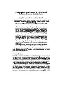
FIGURE 1. Message Sequence Chart for the Remote Interface Controller scenario
The initial state of the software design, before configuration begins, can be in various forms; here it will be described by a set of Message Sequence Charts (MSCs) showing the scenarios, and alternatively by a Collaboration Diagram (part of UML [1]) showing the interacting objects. In either case it will be captured in a model with architectural and performance features, called a Layered System Model, which corresponds closely to a performance model called a Layered Queuing Network or LQN [7][17][24][26].
objects in the system, the arrows are for messages between objects, and the boxes are for activities executed within an object. The leftmost bar in the Figure represents the environment of the system, sending a start event to the Control task which in turn initializes the Monitor, triggers its logging function, and commands the remote interface task to take the sample.
The scenario illustrated by the MSC in Figure 1 “Control” describes a Remote Interface Controller which activates a remote interface with a monitor and an actuator, which in turn takes a sample value of an environmental measure and returns it, as well as logging the request locally. The vertical bars represent locations or
The Layered Queueing Network Model (LQN) shown in Figure 2 describes the software at the level of concurrent tasks that offer different services, or (equally) as active objects that offer different methods to their client objects. It embeds the sequence detail from the MSC or the collaboration diagram within the objects, redraws
input stream ENV (the reply to get_sample should arrive within Ds sec.)
get_sample Control Task m0
a1
sample_done, reply to ENV
a4 m8
init
init_done b2
b1
init entry
m5
m1
start entry Monitor Task
a3
m3
a2
log entry m4
actuate
m2 I/F Control
ckpt
Legend
actuate entry
Synchronous request Asynchronous message Forwarded request
c1
c2
m6
entry ckpt sample
Reply message x
Computation activity Communication activity
d1
d1
Actuator Task m7 (reply to start entry, activity m5)
sample entry
FIGURE 2. Layered Queueing Network Model for the Remote Interface Controller
ENV-1
ENV-2
stim1
stim2
Task A
Task D
Legend Synchronous request
a1 m1
d1 m4
m2
Asynchronous message Forwarded RPC
Task B b1 m3
CPU1
a1
Computation activity
Task E
Communication activity prio(A) = 1 prio(B) = 1 prio(C) = 1 prio(D) = 2 prio(E) = 2
e1
Task C
entry E1 c1 entry C1
c2
entry C2
CPU2
Message Cost: stim1=0, stim2=0 m1=0, m2=0 m3=0, m4=0
Activity Cost a1=12 b1=15 c2=15 d1=18
c1=30 e1=10
Period(stim1) = 70
period(stim2) = 70
Perf. Requirements: deadline(stim1) = 60
deadline(stim2) = 70
FIGURE 3. LQN model for an example with two scenarios them as concurrent tasks represented by parallelograms, and identifies an entry within each task for each different message it accepts during the scenario. The activities in the MSC (labelled a1, b2, etc.) are attached in Figure 2 to the entry which triggers them within each task, along with dummy activities (labelled m1, m2, etc.) which are introduced to send messages and receive replies. The activities are connected by predecessor/successor arcs into the LQN connectors, so for instance the path in Control forks three ways after m3, one path being an asynchronous message to Monitor, the other two triggering a3 and m5. This is an AND-fork. It is also possible to have an AND-join, OR-fork connectors such that one of the output paths is triggered, OR-join connectors, and loops, although these are not shown in the example. The notation used in Figure 2 for sequences of operations is conventional, and is much like the execution graph defined in [19] or the task graph defined in [22] and many other works. The only unusual aspect is that activities may send messages to other tasks, but here we have kept message activities separate from activities which do work. The intertask arrows represent three kinds of interactions, labelled on Figure 2: synchronous (send-reply) interactions have solid arrowheads (with the replies indicated by incomplete short arrows with open heads), asynchronous messages have open arrowheads, and forwarding interactions have a dashedstyle of line and a solid arrowhead. Forwarding interactions are a feature of the LQN framework which describe a task which sends a message and waits for a reply, but the request is forwarded from one server to the next before a reply is sent directly back to the originator. An Environment task is provided to drive the scenario, and to receive the response at the end, and this task is driven by a stream of input events as shown in Figure 2. An LQN may combine several scenarios from several MSCs. Figure 3 shows a system with two scenarios, driven by environment tasks ENV-1 and ENV-2. The rest of the tasks are merged (that is, if a task with the same name appears in two scenarios it is assumed
to be the same task). A separate entry is included for each different message received by a task, illustrated here by the two entries C1 and C2.
2.2 Evaluation of configuration performance The Configuration Planner takes the software description and a description of the execution environment, and configures the software into the environment. The present version assumes a set of processors (not necessarily homogeneous) connected by a single communications fabric with a characteristic delay. It assumes known CPU demands for communications overhead, which is a function of the messages being passed, and of whether the message is local or remote. Tasks will have fixed pre-emptive priorities, a commonly used priority strategy in real-time kernels. The goal of configuration is to satisfy response time constraints for each scenario. The response delay Ts to each arrival event in scenario s should be less than a desired delay Ds, in at least a given percentage of cases. In the MSC the response completion will always be indicated by a reply to the environment (even if the software does not actually send a message), which should arrive within delay Ds. The LQN was evaluated for the probability Ps: Delay Requirement:
P s = Prob { T > D
s
s } < ps
(1)
An example could be P1 = Prob {T1 > 300 msec } < 0.05, for a scenario numbered as 1. For hard deadlines the probability ps is set to zero. For soft deadlines, characteristic of telecommunications systems, it might be 0.05 or 0.01. For hard deadlines a value of Ps greatter than 0 indicates that the response targets have not (yet) been met and further search is needed to get a satisfactory configuration. This work will consider only hard deadlines, but the Planner is adaptable to soft deadlines as well, by using a larger value of
Node 3 Node 15
Node 1 Node 2
Node 16
Sub-node A
Sub-node B
MH MH
FH
PFSM
CTRL
SM
RT
SQM
AM
AM
SM
CTRL
SQM
RT
FH
PFSM
Shows flow of messages if protection request comes from left (I.e. from Node 16) Shows flow of messages if protection request comes from right (I.e. from Node 2)
FIGURE 4. A 16-node optical ring and protection swtiching system, showing the two processors for node 1, and the activities they perform. The dashed arrows in this diagram show parts of Scenario 1 propagated around the ring from the right (solid arrows, from the left). ps.
3.1 Initial Allocation
There is a stream of arrival events for each scenario, with a known average arrival rate. These arrivals may be periodic, with a fixed arrival period, or may have a random inter-arrival interval.
The initial allocation of tasks to processors was found using MULTIFIT-COM [25], an algorithm for optimal allocation of tasks with execution and communications demands, to a homogeneous set of processors. MULTIFIT-COM was used because it was shown in [25] to be robust and quick compared to competing algorithms, and to scale well. It balances the load between processors, which is agreed to be generally favorable to schedulability [3][11][18]. It extends the bin-packing approach of MULTIFIT [2] to account for communications costs.
2.3 A Protection Switching System A typical application is the protection switching software for a BLSR (Bidirectional Line Switching Ring, an optical ring configuration), shown in Figure 4. It has 16 nodes with two processors each, and 256 activities altogether, although the 16 nodes may be assumed to be symmetrical. For a single failure on a ring with less than 1200 km. of fiber, the protection operation should propagate knowledge of the failure, and re-route all traffic to use the remaining connectivity, in less than 50 msec. Although nodes react in a symmetrical fashion, there were three different scenarios to be considered depending on how far from the node the failure occurs (the nearest neighbour in the traffic direction, giving Scenario 1 shown in Figure 4, nearest in the other direction, and elsewhere). The LQN for a fault occurring to the left of Node 1 is shown in Figure 5. Space does not permit showing the full model, however the Figure does show that there are many complex tasks, and tasks which participate in multiple scenarios.
3.0 THE INITIAL CONFIGURATION The initial configuration is an allocation of tasks to processors, determined by a simple heuristic allocator, and an initial set of priorities determined by a simple heuristic rule. Once established and evaluated, the configuration is then iteratively improved, as described in Section 4.
MULTIFIT-COM requires knowledge of the execution demand of each task and of the communications overhead between each pair of tasks (when not co-located), in executing one scenario. The present situation is a little more complex, since there are multiple scenarios being executed concurrently. Here the scenarios are combined, taking advantage of the fact that the rates of activation of the scenarios are all assumed to be known. The average rate fe of messages to each entry e can be found by summing up the number of messages to entry e within each scenario, times the activation rate of the scenario. Then the processor utilization Ue imposed by the entry is fe times the sum of the activity demands for entry e, and the processor utilization of task t is the sum of the entry values: Ue = f e
∑ E a,
a∈e
Ut =
∑ Ue
e∈t
Similarly the CPU utilization to send or to receive messages that go between entries d and e (when they are on separate processors) is the product of the frequency fde of these messages, and the execution demand Ede per message. The communications load between tasks is the sum over the entries at both ends. Thus:
Fault Generator
FH
FH
PFSM
FH
PFSM MH
FH
T1
FH
PFSM
PFSM
CTRL
CTRL
FH
T1
PFSM
PFSM
MH
CTRL
CTRL
CTRL
CTRL MH
SM
SM SQM
SQM
SM
AM
AM
MH
AM
Subnode A
Subnode B
SM
SQM RT
Subnode A
Node1
MH
SQM
AM
Subnode B
RT
SM
MH SM
SQM
SQM
AM
AM
Subnode A
Node2 - Node15
Subnode B
Node16
Legend Synchronous message
Reply message
Asynchronous message Forwarding message
FIGURE 5. The Layered System Model for the Protection Switching Software.
U de = f de E de,
U tu =
∑
d ∈ t, e ∈ u
U de
Now suppose the value of Utu found for local communications (when t and u are allocated to the same processor) is U*tu, and the value for remote communications is U**tu. The penalty for separate allocation is then ∆Utu = U**tu - U*tu. In these calculations each individual activity has its own execution demand Ea which contributes to Ue and thus to Ut, and each message has its own size parameters which determine its contribution to the execution demand Ede and thus to Utu and to ∆Utu. There is no restriction to homogeneous activities or messages. With this notation the MULTIFIT-COM algorithm is adapted to the present problem as follows:
•
the “execution cost” of a task t was taken as Ut + ΣuU*tu, the expected total utilization of its entries by all scenarios plus the local communications overhead (the minimum value for communications overhead), • the “communications cost” between a pair of tasks t and u, when they are allocated to different processors, was taken as ∆Utu. MULTIFIT-COM combines the results of a variety of policies to order the tasks and the bins (processors) and to decide how to pack the bins. In this work eight different policies were used. Instead of just taking the best solution as in [25], eight possibly different starting points were passed to the improvement algorithm described below. The seven policies selected by the extensive sta-
tistical evaluation in [25] were used, plus one more which appeared to be useful for this variation of the problem (as identified in [25], these are strategies numbered 2,4,6,8,10,12,13 and 19). It should be noted that, unlike some other methods (including the methods of [18] and [22]), MULTIFIT-COM does not take into account memory size constraints. Memory is not as important as fact or as it was once, and we feel that additional memory can be added if the configuration demands it.
3.2 Initial Priorities Given an initial allocation, the initial priorities on each processor were determined by the proportional deadline method of Sun et al. [21]. The deadline value of an entry is a part of the deadline of its scenario, proportional to the average execution demand of the entry per scenario repetition. The task deadline value is a weighted average of entry values weighted by their relative frequency. The task priority is based on the estimated laxity, calculated as the difference between the deadline value and the weighted average demand (in which entry demands are weighted in the same way, by entry frequency).
3.3 Evaluation of the Initial Configuration Given the initial configuration, the ability of the system to meet its deadlines can be evaluated. The approach taken was to simulate the system, record the occurrence of deadline hits and misses, and estimate the metric Q, as follows. Deadline misses are measured by a quantity S(s), which captures how far scenario s is from its delay target. S(s) is zero for a scenario which meets its specification, and increases as Ps defined in
sages, which might become inter-processor messages. This sum is then multiplied by the cost c of an interprocessor message:
Eq. (1) increases; in this work the function used for S(s) was
Ps ≤ ps
S ( s ) = 0,
(2) S(s)
= exp (βP s),
( Ps > ps )
The definition of S(s) (with some arbitrary positive value of β)was chosen to penalize all misses, and to give accelerating importance to the penalty as the probability of missed deadlines increases beyond the permitted level ps. The overall quality of a configuration is then measured by the sum Q =
∑ S(s)
(3)
s
and a configuration which meets its timing requirements for all scenarios has Q = 0.
3.4 Task ranking The goal of improvement is to satisfy the timing constraint of Eq. (1) for all the deadline targets. If some target is not met, the improvement algorithm ranks the tasks, and then attempts to make changes, beginning with the highest ranking task. After one successful change, the constraints are checked and if necessary, the ranking is done again. The ranking metric RTASK(t) indicates the contributions of task t to delay in all the scenarios that miss their deadlines, by way of the following sum: 1 R TASK ( t ) = --------------------------U TASK ( t )
∑ S ( s )w1( s, t ) s
in which UTASK(t) is the utilization by task t of its processor, and S(s) is given in Eq. (2). The factor 1/UTASK(t) was introduced because experience showed it is useful to raise the rank of lightly loaded tasks. The weight w1(s,t) is roughly the delay that task t introduces into scenario s, which might be reduced by changing the priorities and allocations. It was found as w 1 ( s, t ) = W ( s, t ) + ∆C ( s, t ) where
• •
W(s,t) is the contribution to the critical path of scenario s, made by the waiting time of task t for its processor (expressed as mean wait time per response) ∆C(s,t) estimates the decrease that might occur in delays due to communications overheads, if task t were moved to another processor, and local messages on the same processor are taken as “free”. It does this by counting the number of remote messages from t per response, and per other processor, which might conceivably disappear in a reallocation, and subtracting the number of local mes-
∆C ( s, t ) =
∑
∑
cm cm – m ∈ Remote ( t ) ------------------------------------m ∈ Localt Nremote ( t )
with P being the number of processors, Local(t) being the set of messages between task t and all other tasks on the same processor, Remote(t) being the set of messages involving the P-1 other processors, and Nremote(t) being the number of processors with tasks that communicate with task t. The cost cm of a message may be different for each message m, for instance from the message size. The tasks with RTASK > 0 are now ranked in order of the value of RTASK, with the Candidate task t* being the one satisfying: R TASK ( t∗ ) =
max { R TASK ( t ) } t
This task has the greatest potential to improve the overall meeting of deadlines. If only one scenario fails to meet its deadline, only tasks which participate in that scenario will have a non-zero score R, and one of them will be the Candidate task.
3.5 Making the configuration change steps Having found the highest ranking task t*, the following changes are considered, in this order: a) increase the priority of t* by one step, on its processor, as described in Section 3.6. b) re-allocate it to another processor, the one that is least stressed, according to the CPU metric RCPU defined below in Section 3.7; reset the priorities on this processor using the Initial Priority rule in Section 3.2. c) split the task, dividing its functionality between two tasks, as described in Section 3.8. This may then permit priorities to discriminate between critical and non-critical functions of the same task, and indicates that the clustering of these functions within the same task is a poor choice at least for performance reasons. Note that dividing the task like this is a hypothetical change, made in the model and evaluated as an indication to the designer; in fact the task may not be divisible in this way. These three changes are considered in the order of difficulty required to achieve them in practice. A priority change is relatively simple to carry out, an allocation change is more difficult but at least keeps the design intact, and a task splitting requires some software redesign. The Planner algorithm can be summarized as follows: 1. Initialize the configuration 2. Evaluate the configuration by simulating the model, and if the deadline requirements are met, the algorithm stops with condition SUCCESS. If the requirements are not met but the solution quality metric Q has decreased, the previous step is said to have succeeded. 3. Try a priority change as in a) above, followed by step 2, unless the Candidate Task t* already has the highest priority, or six
successive priority changes have failed to give any improvement in Q. In these cases pass on to step 4. 4. Try re-allocation of task t*, as in b) above, followed by step 2, unless • t* has already been re-allocated (with no successful priority steps since then), • it is not permissible to re-allocate t*, due to allocation constraints, • the target processor utilization would then exceed 0.95. If re-allocation is not permitted pass on to step 5. 5. Split t* as in c) above, followed by step 2; if this is impossible (for instance it may have only one entry), pass on to step 6 6. Consider the next-ranked task to be t*, and go to step 3. If the list of tasks with RTASK > 0 is exhausted, exit the algorithm with condition FAILURE.
3.6 Priority changes One task priority is changed at a time, by increasing the priority of the highest ranking task by one step. A step is related to the priority groups on each processor, within which the tasks have equal priority. When a task is moved up one priority step, if it is in a group with other tasks then it moves into a new group created to hold it, between its old group and the one above. If it is in a group by itself, it joins the next group up. To show the operation of the priority change steps, the example of Figure 3 was adjusted to have a poorly chosen initial set of priorities, which gave unsatisfactory delays (after the actual initialization step produced a satisfactory configuration at once). In this case priority change steps alone were enough to give a satisfactory configuration, as shown in Table 1.
TABLE 1. Priority changes for the system of Figure 3, from first modified starting point Step
t*
Action
T1, T2
P1, P2
Q Eq. (3)
Initial configuration as Figure 3
70.004, 28.0
1.0, 0
3269017
70.004, 28.0
1.0, 0
3269017
1
A
CPU1 priorities change from
2
A
CPU1 priorities to: (D, A) > B
70.004, 28.011
1.0, 0
3269017
3
A
CPU1 priorities to: A > D > B
67.0, 40.0
1.0, 0
3269017
4
B
CPU1 priorities to: A > (D, B)
67.0, 40.0
1.0, 0
3269017
5
B
CPU1 priorities to: A > B > D
67.0, 55.0
1.0, 0
3269017
6
C
CPU2 priorities from E>C to (E,C)
57.0, 67.0
0, 0
0: SUCCESS
D > (A, B) to: D > A > B
3.7 Re-allocation A re-allocation step moves only the Candidate task t* from its present processor to a target processor p*, which is chosen as having the least contribution to deadline failure. The target processor is found by ranking the processors according to the metric RCPU(p): R CPU ( p ) = U ( p )
∑ RTASK ( t )
t∈p
in which U(p) is the utilization of processor p and RTASK(t) is the ranking measure of a task t running on processor p. The candidate processor p* is the one with the smallest value of RCPU(p): R CPU ( p∗ ) =
min p
{ R CPU ( p ) }
In this sense, the other tasks on p* contribute the least to deadline failures and presumably have the greatest tolerance for competition from t*.
To show how the Configuration Planner arrives at a re-allocation step, a second poorly chosen starting point was imposed on the system of Figure 3, giving the steps shown in Table 2. Priority changes are only rejected when no new step can be taken, or the candidate task is the highest in priority already. CPU1 is chosen for the re-allocation because of its utilization. Priority was set equal to the highest-priority task that it communicates with, or to the maximum priority on the new processor.
3.8 Task Splitting The rationale for task splitting is that a task may combine urgent operations with others that are not. If the task can only do one operation at a time, then a more-urgent request may be waiting in the message queue while a less-urgent operation is being performed, which is a form of priority inversion. Separating the entries into separate tasks means that a higher priority can be given to the more urgent operations. Splitting in this way assumes that the distinction in urgency is associated with different entries in the task. If more and less urgent streams of requests arrive at the same operation, the operation itself can in some cases be split into two entries, which do the same functional operation for different requests. Then the splitting can proceed. Some tasks cannot be split, because for example all the entries may update a single data structure, so the task acts as a critical section.
TABLE 2. Configuration changes for the system of Figure 3,showing re-allocation, from second modified starting point step
t*
Action
T1, T2
Priority: from D > (A, B) to D > A > B
P1, P2
Q Eq. (3)
70.0, 30.0
1.0, 0
3269017
70.0, 30.0
1.0, 0
3269017
1
A
2
A
Priority: to (D, A) > B
71.36, 30.30
1.0, 0
3269017
3
C
Priority: from E > C to (E, C)
70.02, 36.54
1.0, 0
3269017
4
C
Priority: to C > E
77.50, 77.51
1.0, 1.0
6538034
5
E
...Try priority (E, C), but this has been visited before; 70.02, 40.0 ...Try priority E > C , but this has been visited before; ...t* has highest priority SO reallocate candidate task E to CPU1 with priority order: (E, D, A) > B
1.0, 0
3269017
6
A
Priority: to A > (E, D) > B
70.0, 41.0
1.0, 0
3269017
7
B
Priority: to A > (E, D, B)
70.0, 56.0
1.0, 0
3269017
8
B
Priority: to A > B > (E, D)
59.0, 57.0
0, 0
0
To identify the task to be split and the entry to be split off, the entries in task t* were ranked by a measure RENTRY(e) which combines the criticality of the scenario with the delay contribution of the entry to that scenario. R ENTRY ( e ) =
∑ W ( s, e )S ( s )
entry e* is the one with the largest value of RENTRY(e): R ENTRY ( e∗ ) =
max { R ENTRY ( e ) ( e ∈ t∗ ) } e
and a new task is made with one entry e*, and priority one step above the old task t*, allocated to the same processor. The task t* has the entry e* removed from it.
s
in which s is the scenario containing the entry e, and W(s,e) is the processor waiting contributed by activities of e to the critical path of scenario s (i.e. that part of W(s,t) due to entry e). The candidate
To show the operation of task splitting, a different poorly chosen starting point was imposed on the example in Figure 3, giving the evolution shown in Table 3. There are a number of steps taken
TABLE 3. Configuration changes of the system of Figure 3 showing task splitting Step
t*
Action
T1, T2
0
P1, P2
Q, Eq. (3)
70.00, 28.00
1.0, 0
3269017
1
A
Priority: from D>(A,B) to D > A > B
70.00, 28.00
1.0, 0
3269017
2
A
Priority: to (D,A) > B
70.004,28.011
1.0, 0
3269017
3
A
Priority: to A > D > B
72.41, 32.61
1.0, 0
3269017
4
B
Priority: to A > (D, B)
72.34, 34.52
1.0, 0
3269017
5
B
Priority: to A > B > D
72.34, 41.26
1.0, 0
3269017
6
C
Priority: from E > C to (E, C)
62.00, 69.14
1.0, 0,001
3269018
7
C
Priority: to C > E
62.00, 69.14
1.0, 0.001
3269018
8
C
Task C has highest priority Reallocating task C to CPU1 gives utilization > 0.95. SO: Split candidate task into C_1, C_2 new priority order: C_1 > C_2 > E
47.00, 69.14
0, 0.001
1.013
9
E
Priority: to C_1 > (C_2, E)
47.00, 69.14
0, 0.001
1.013
10
E
Priority: to C_1 > E > C_2
47.00, 57.00
0, 0
0
before task splitting is forced. First, re-allocation must be rejected, which happens at step 5 because it leads to excessive utilization.
4.0 EXPERIENCE Three forms of experience will be described as evidence that the Configuration Planner is robust and effective: the Protection Switching system, a system of simple tasks, and a large set of ran-
Period = 60 T0 [4]
0
T1 [4] 60 70 30 T3 [2]
1
T5 [4] 60
T4 [2] 80
T6 [6]
2
Period = 14
Period = 14
T24 [1]
20
T31 [2] 70
T26 [1] 20
T27 [1]
T32 [2] 7
T28 [1] 30
T10 [14]
250 T11 [4] 1
T17 [2]
2
T34 [2] 2,3
50 T35 [2] 60 60
50
T36 [2] 2,3
T37 [2]
T20 [1] 40
T19 [1] 1
T21 [2] 3
Period = 20
Period = 20 T33 [3] 2,3
Period = 14
50
50
T14 [2] 50 50 T15 [2] 3
T30 [1] 7 50
20 T25 [1]
0
Period = 14 Period = 35 T18 [1] 1 T16 [2] 3
T12 [2] 2 150 150
40
T29 [1]
90
T13 [2]
T23 [1]
50
T9 [8]
1
T8 [2]
20
40
Period = 35
40
T2 [2]
T22 [1]
20
1
T7 [2]
150
50
Period = 14
Period = 35
T38 [3] 3,2
T39 [2] 1,0 50
50 T40 [2] 60 T41 [2] 7,6
60 T42 [2]
6
FIGURE 6. The 11 scenarios in the system studied by Tindall et al, and Santos et al, showing the activities (named Ti for i = 0 to 42), their CPU demands in msec, their precedence relationships, and the message sizes in bytes. domly chosen systems with complex tasks.
4.1 Protection Switching System results A realistic set of execution demands for the tasks in Figure 5 were used in the study. Much of the initial configuration of this system was constrained by imposed symmetry of the 16 nodes, and of allocation on the two processors in each node. Only the priorities remained to be chosen, and the initial priorities chosen by MULTIFIT-COM were satisfactory. When a poor set of priorities was imposed as an artificial starting point, the algorithm found a satisfactory set of priorities in just three steps.
4.2 Tindell/Santos example Asystem of simple tasks of the classic form was described by Tindell et al. in [22]. They and Santos et al. [18] described heuristic algorithms for task allocations and priority assignments. As shown in Figure 6 the system has 43 activities in 11 periodic scenarios with deadlines equal to their periods, and eight processors. There is a propagation delay of 1 msec for interprocessor messages, and communications overhead demand was set to zero. About half the tasks are constrained to allocation to a particular processor, indicated by processor numbers in small boxes to the right of the task. This system was translated into an LQN with one task per activity, and with the precedence of activities maintained. Eight initial configurations with five distinct solutions were found. The Planner succeeded in finding successful configurations from all eight starting points. It took an average of four steps to succeed. Thus, apart from the fact that it does not respect certain memory constraints, it is just as successful as the algorithms in [22] and [18].
In this base case (we may call it Case TS0) there were 8 processors and communications overhead demand was zero. To extend the evaluation, the difficulty of the configuration problem was increased in four successive additional experiments: Case TS1: A CPU overhead of 1 microsec/byte was included for interprocessor messages, for both the sender and receiver. All eight trials succeeded, in an average of 16 steps. Case TS2: The messaging overhead was increased to 3 microsec per byte. Now only 7 out of 8 optimization trials succeeded, and those took an average of 23 steps. Case TS3: The number of processors was reduced from 8 to 7 and the messaging overhead set to zero. Now 6 out of 8 trials succeeded, and those took an average of 26 steps. Case TS4: With 7 processors the messaging overhead was set to 1 microsec/byte. Now 5 out of 8 trials succeeded, and those took an average of 51 steps. The Configuration Planner appears to tackle these more difficult problems in a robust way, and does not bog down completely. The variety of starting points appears to be a strength.
4.3 Statistical evaluation The effectiveness of the Planner on more difficult systems with complex (multi-entry, multi-activity) tasks, which are shared between scenarios, was evaluated on a large sample of systems with randomly generated parameters and graded levels of difficulty. Two fixed software architectures were designed, of which Figure 6 shows one; each architecture had four scenarios and 16 tasks (of which 11 participate in more than one scenario), and tasks send an average of 1.3 messages during a scenario. The determin-
FIGURE 7. LQN structural template used for half of the statistical evaluation cases
istic execution demands were selected randomly for each entry, from the range [80,120]. Then in each case two factors L and U were chosen to adjust the difficulty of the configuration task. L is a laxity factor, such that the deadline of each scenario was set to give: D = demand × L , where demand estimates the CPU s s demand of the scenario and L took values between 2.1 and 3.0. U is the average processor utilization, and determined the period of each scenario as Period = demand × U . U took values s s between 0.4 and 0.8. A large value of U gives less contention and an easier configuration problem; similarly a large value of L makes deadlines easier to achieve. Although the use of the L and U factors tends to define systems whose execution can be fitted into the deadlines, random variation can make a scenario critical path longer than its deadline, and these cases were deleted and replaced. Contention and precedence can still make some of the remaining cases unschedulable, however. Five values of L and five of U gave 25 combinations, and for each of these, 60 cases were generated randomly, to give 1500 cases for each architecture, and 3000 cases in all. The ratio of feasible (successful) cases x out of a given y cases, (where none of the y cases are obviously infeasible) gives the Success Ratio (SR) (x/y). The results in Figure 8 and Figure 9 show that success is favored
FIGURE 9. Number of steps required to find a satisfactory configuration, for those trials which ended in success, against the CPU utilization factor F and the laxity factor L. by larger L and smaller U, which is only reasonable; they indicate that a laxity factor of about 3 is enough to give success almost always, and in a moderate number of steps. It appears from the results that the strategy and heuristics used for optimization are robust and guide the algorithm efficiently for a feasible design. For example, the optimization method succeeded in finding a feasible solution more than 80% of the time when the Laxity factor was 2.6 or greater, or the average CPU utilization was less than 50%. In addition, when the average CPU utilization was around 60%, the optimization method only performed 20 steps on average to find a feasible process allocation and priority assignment to the software design. Even when the average CPU utilization was as high as 80%, the optimization method only performed 35 steps on average to find a feasible solution.
5.0 CONCLUSIONS The heuristic Configuration Planner described here determines allocations and priorities and may split tasks, to achieve deadline requirements on delays. It assumes fixed pre-emptive priorities, homogeneous processors, and it ignores memory constraints. It executes quickly, and it has succeeded in solving a wide range of configuration problems. The Planner addresses systems with more realistic software structures and architectures than heretofore studied, including what are called complex tasks, with multiple entries, which participate in multiple scenarios. The realistic system for protection switching is an example of complex tasks, but it turned out to have an easy solution. A range of synthetic problems were more difficult, including a large system of simple tasks and many large systems of complex tasks.
FIGURE 8. Success Ratio for statistical evaluation, against CPU utilization factor F, for different values of the laxity factor L
The statistical evaluation suggests that ease of configurability may be understood in terms of average utilization and a laxity factor. The results suggest that a combination of an overall utilization around 0.6 and an average laxity factor of about 2.3 is almost always configurable. These measures need to be tested on additional architectures, but they provide an interesting direction for further investigation. The testing of the Planner described here is for hard real-time
response requirements, because of the background of the project, and the larger number of studies for comparison. However the measure Q of satisfaction of requirements is equally well adapted to soft real-time deadlines, and the Planner should be equally effective on them; this is the subject of further work. References [1] G. Booch, J. Rumbaugh, I. Jacobson, The Unified Modeling Language User Guide, Addison Wesley, 1998. [2] E.G. Coffman, M.R. Garey and D.S. Johnson, “An application of bin-packing to multiprocessor scheduling”, SIAM J. Comput., vol. 7, pp. 1-17, Feb. 1978. [3] Wesley W. Chu and L. M. Lau, “Task allocation and precedence relations for distributed real-time systems”, IEEE transactions on Computers, 36(6):667-679, June 1987. [4] S.K. Dhall and C.L. Liu, “On a real-time scheduling problem”, in Operations Research, vol. 26(1), pp. 127-140, Feb. 1978 [5] H.M. El-Sayed, D. Cameron, and C.M. Woodside, “Automated performance modeling from scenarios and SDL designs of distributed systems”, In Proc. of the Int. Symposium on Software Engineering for Parallel and Distributed Systems (PDSE’98), Kyoto, April 1998. [6] R. Etemadi, G. Karam, S. Majumdar, “Heuristic algorithms for priority assignment in flow shops”, Proc. Int Conf. on Performance, Computing and Communications (IPCCC98), pp 15 - 22, 1998. [7] G. Franks, A. Hubbard, S. Majumdar, D. Petriu, J. Rolia, and C.M. Woodside, “A toolset for performance engineering and software design of client-server systems”, Performance Evaluation, 24 (1-2):117-135, Nov. 1995. [8] J.J.G. Garcia and M. Gonzalez Harbour, “Optimized priority assignment for task and messages in distributed hard realtime systems”, Proc. of the IEEE Workshop on Parallel and Distributed Real-Time Systems, California, pp. 124132, April 1995. [9] F. Hoeben, “Using UML Models for Performance Calculation”, Proc. of Second International Workshop on Software and Performance (WOSP2000), pp. 77-82, September, 2000. [10] C.J. Hou and K.G. Shin, “Allocation of periodic task modules with precedence and dead-line constraints in distributed real-time systems”, in Proc. of the Real-time system symposium, pp. 146-155, 1992 [11] C.E. Houstis, “Module allocation of real-time applications for distributed systems”, IEEE Transactions on Software Engineering, vol. 16, pp. 699-709, July 1990. [12] P. Kahkipuro, “UML Based Performance Modeling Framework for Object-Oriented Distributed Systems”, Proc. of UML 99, LNCS, Springer Verlag, vol. 1723, pp. 356-371, 1999. [13] J. Lehoczky, L. Sha, and Y. Ding, “The rate monotonic scheduling algorithms: exact characterization and average case behavior”, In Proc. of the 10th IEEE Real-Time Systems Symposium, pp. 166-171, 1989. [14] C.L. Liu and J.W. Layland, “Scheduling algorithms for multiprogramming in a hard real-time environment”, in Journal of the Assoc. Computing Mach., vol. 20(1), pp. 46-61, 1973.
[15] D-T. Peng, K.G. Shin, T.F. Abdelzaher, “Assignment and scheduling communicating periodic tasks in distributed real-time systems” , IEEE Trans. on Software Engineering, v 23, n 12, Dec 1997. [16] K. Ramamritham, “Allocation and scheduling of precedencerelated periodic tasks”, IEEE Transactions on Parallel and Distributed Systems, 6(4): 412-420, April 1995. [17] J. R. Rolia and Kenneth Sevcik, “The method of layers”, IEEE Transactions on Software Engineering, Vol. 21, No. 8, pp. 689-700, 1995. [18] J. Santos, E. Ferro, J. Orozco, and R. Cayssials, “A heuristic approach to the multitask-multiprocessor assignment problem using the empty-slots method and rate monotonic scheduling”. Real-Time Systems, 13, 167-199 (1997). [19] C.U. Smith, Performance Engineering of Software Systems, Addison-Wesley Publishing Co., New York, NY, 1990. [20] M.F. Storch and J.W.S. Liu, “Heuristic algorithms for periodic job assignment”, In Proceedings of the Workshop on Parallel and Distributed Real-time Systems, pp. 245-251, Apr. 1993. [21] Jun Sun, Fixed Periodic Scheduling of Periodic Tasks with End-To-End Deadlines, Ph.D. thesis, Department of Computer Science, University of Illinois at Urbana-Champaign, Urbana, Illinois, USA, 1996. [22] K.W. Tindell, A. Burns, and A.J. Wellings, “Allocating hard real-time tasks: an NP-hard problem made easy”, RealTime Systems, 4(2):145-165, June 1992. [23] L. G. Williams, C.U. Smith, “Performance Engineering of Software Architectures”, Proc of First Workshop on Software and Performance (WOSP98), Santa Fe, Oct. 1998. [24] C.M. Woodside, “Throughput calculation for basic stochastic rendezvous networks”, Performance Evaluation, Vol. 9, No. 2, pp. 143-160, 1989. [25] C.M. Woodside and G.M. Monforton, “Fast allocation of processes in distributed and parallel systems”, IEEE Transactions on Parallel and Distributed Systems, vol. 4, no. 2, Feb. 1993. [26] C. M. Woodside, J. E. Neilson, D. C. Petriu, and S. Majumdar, “The stochastic rendezvous network model for performance of synchronous client-server-like distributed software”, IEEE Transactions on Computers, 44(1):20-34, January 1995.