has multiple sensors connected to a single laptop which computes the sensor data ... All the computation is performed in one off the shelf notebook computer.
Autonomous Robot Navigation in Outdoor Cluttered Pedestrian Walkways Yoichi Morales, Alexander Carballo, Eijiro Takeuchi, Atsushi Aburadani and Takashi Tsubouchi Graduate School of Systems and Information Engineering University of Tsukuba, Intelligent Robot Laboratory 1-1-1 Tennoudai Tsukuba 305-8573, Japan {yoichi,alexandr,etake,abura,tsubo}@roboken.esys.tsukuba.ac.jp
Abstract This paper describes an implementation of a mobile robot system for autonomous navigation in outdoor concurred walkways. The task was to navigate through non-modified pedestrian paths with people and bicycles passing by. The robot has multiple redundant sensors which include wheel encoders, an IMU, a DGPS and four laser scanner sensors. All the computation was done in a single laptop computer. A previously constructed map containing waypoints and landmarks for position correction is given to the robot. The robot system’s perception, road extraction and motion planning are detailed. The system was used and tested in a 1 km autonomous robot navigation challenge held in the City of Tsukuba, Japan named “Tsukuba Challenge 2007”. The proposed approach proved to be robust for outdoor navigation in cluttered and crowded walkways, first in campus paths and then running the challenge course multiple times between trials and the challenge final. The paper reports experimental results and overall performance of the system. Finally the lessons learned are discussed. The main contribution of this work is the report of a system integration approach for autonomous outdoor navigation and its evaluation.
1
Introduction
Reliable outdoor autonomous navigation is still a major challenge in robotics. The dynamic conditions of outdoor environments such as weather, illumination and vegetation characteristic changes make difficult to build a system that can robustly navigate all the time in all conditions. The motivation of this work is to build a self contained mobile robot capable of navigating in cluttered pedestrian paths which have not been modified for robot navigation. That implies that the robot has to deal with the conditions and hazards present in real outdoor paths. In this work, walkways are defined as paved roads which have irregular form and width (from 1.5 m to 5 m) containing some gentle slopes. The roads are delimited
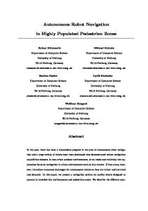
mainly by curbs, however some sections have no specific limits, though in direct contact with rough or grassy unpaved sections. Typical walkway scenes are shown in Figure 1. The walkways considered in this work are mainly surrounded by bushes and trees and there are no crossroads or traffic lights. The static hazards of the environment are: different types of road surfaces, irregular shapes in the road edges, standing pedestrians, parked bicycles, bumps, slopes, stairs. The dynamic hazards are walking pedestrians, passing bicycles, fallen leaves and branches, rain, standing water and change of vegetation characteristics according to the season of the year. The contribution of this paper is the proposal, development and evaluation of a multisensor redundant mobile robot system for autonomous navigation in the previously described walkways. The robot main characteristics are its simplicity in hardware and software. The robot has multiple sensors connected to a single laptop which computes the sensor data processing and motion planning in a distributed software framework.
Figure 1: Typical scenes of walkways in the city of Tsukuba. The main walkway path runs from south to north of the city having an approximate length of 10 km and is used by pedestrians and bicycles. The scientific challenge of this work is to navigate in outdoor paths. To do so, the robot has to sense, extract and process data in real time to compute its position and the path it should follow to achieve its goal while detecting and avoiding obstacles and running out of the road. To be able to interact naturally between people in its surroundings, the robot should move at human walking speeds (0.7 to 1 m/s) as much as possible. Moreover, robots running in transited pedestrian walkways grab the attention of people around, therefore, an effective framework of obstacle detection and avoidance to avoid collisions at any cost is necessary. Detection of traversable and non-traversable areas represented a technical challenge because of the dynamic conditions of the road (such as fallen leaves or branches). The system robustness and performance was evaluated extensively in outdoor walkways. The final experiments of this paper were performed in the event of the Tsukuba Challenge 2007 (or ”TC 2007” in the rest of the paper) which was held in Tsukuba city, Japan. The TC 2007 event was the first time such a challenge was held in Japan and it aimed at 1 km autonomous mobile robot navigation in real world conditions. 1.1
The Tsukuba Challenge
On November 2007, the Tsukuba Challenge (TC 2007 in the rest of the paper) took place in a pedestrian path of the City of Tsukuba, Ibaraki prefecture, in Japan. The challenge was to run 1 km autonomously in real outdoor environments that could not be altered or
modified for robot navigation purposes. Figure 1 shows some snaps of the course and Figure 2 shows the top view of the course in Google Maps. In Japan the use of public places for robot navigation without authorization is not allowed. Therefore, for the TC 2007 event, the city’s authorization was granted for robots to share a public walkway with pedestrians and bicycles. Some of the most relevant conditions of the challenge were:
Figure 2: Tsukuba Challenge 2007 path viewed in Google Maps with some snapshots of the course (Tsukuba, 2008) (http://www.robomedia.org/challenge/kadai.html). • There is no cash prize. The objective is to share experiences learned for outdoor robot navigation in real environments. • Regarding the robot regulations, it should be environmentally friendly (no combustion engines allowed) and it should not endanger nor give any sensation of danger to people. Robots should have a stop button and no communication devices between operators were allowed. • Changes (beacons, markers) or restrictions in the environment were not allowed. • It would took place in most weather conditions except heavy rain. There was a total of seven trials from October to November, the qualifying and final runs were held during the 16th and 17th of November respectively. Between universities, research institutes and private participations, a total of thirty three teams were registered into the event. Eleven teams made it to the final where three teams could complete the 1 km run. Our team from the Intelligent Robot Laboratory of the University of Tsukuba finished with the best official time of 23.0 minutes at an average speed of 0.72 m/s.
1.2
Approach
We gave priority to people’s safety; this was to avoid any collision with surrounding obstacles. Interaction between robots did not occur, so no traffic negotiation among robots was required. We took the next issues into consideration: • GPS suffers from signal blockage, multipath and blackouts next to tall obstacles. • In environments with GPS barely available, localization towards a map containing natural landmarks would be required. • Precise localization is a difficult task to accomplish. Therefore a reliable traversable road extraction method to keep the robot in the path is necessary. We built a robot system using existing state of te art that could have the flexibility to cope with the previous requirements. The robot characteristics are: • It is a complementary redundant multisensor system in the sense that when one sensor or approach is not available it could be supported or backed up by another one. • Its distributed multi-process software architecture with inter-process communication capability allowing data sharing of one sensor to several data processing processes. • All the computation is performed in one off the shelf notebook computer. There are several individual approaches for perception, robot localization and motion planning, however, system integration is still an open key issue for having robots interacting in our everyday lives. This work reports our system integration approach for navigating in real walkways. The main characteristics of the system are its simplicity and redundancy in hardware and software. The rest of the paper is organized as follows. In Section 2 related works are presented, Section 3 treats the hardware and software considerations made for the system design, Section 4 explains the terrain classification method, Section 5 details the localization framework, Section 6 explains the navigation approach, Section 7 presents experimental results, discussion and lessons learned are presented in section 8 and finally conclusions and future works are presented in Section 9.
2
Related Works
The problem of successful autonomous robot navigation in cluttered environments have already been reported in previous works. A museum guide robot called Rhino was developed to guide and interact with museum visitors (Burgard et al., 1999). The challenge was to guide visitors of the museum in crowded environments achieving localization and motion planning with obstacle avoidance for navigation. Global localization is based on a Markov multi-hypothesis approach (Fox et al., 1998b) and collision avoidance on the dynamic window approach (Fox et al., 1997). An improved version of the museum robot was Minerva (Thrun et al., 2000), which had to interact in a larger museum and presented an improved robothuman interaction with a face. Our robot did not have web interface nor people interactive components as Rhino or Minerva did, on the contrary, it was a simple self-contained system which operated with a single computer. All software components were computed on-board. An EKF is used for robot localization where a single hypothesis approach kept low the computational load.
Autonomous navigation among pedestrians was reported in (Pradalier et al., 2005) where a car-like robot was developed. The authors mention the difficulty of natural features detection and use cylindrical artificial landmarks combined with a SLAM framework of a car-park area for robot localization. The work is centered in motion planning and the necessity of a framework for perception and identification of obstacles to predict their movement is addressed. In our approach obstacles are detected using information from the laser sensors but we do not treat obstacle recognition problem, thus no movement prediction is done. In (Guivant et al., 2000) the use of natural and artificial landmarks for vehicle localization is treated in a SLAM approach. This two works report the use of artificial landmarks for vehicle localization and its convenience when dealing with data association. In our work natural available landmarks such as road curbs were used as landmarks, so no artificial landmarks were placed. Successful autonomous vehicles driving several kilometers have been already developed in the Grand and Urban Challenges organized by DARPA. In the first Grand Challenge of 2004 no vehicle could run the whole course. In the next year, five vehicles finished the task of running 244 km demonstrating that autonomous long range navigation was feasible using present state of the art (Thrun et al., 2006), (Urmson et al., 2006). In the Urban Challenge held in 2007 six vehicles completed the task of autonomously driving 97 km in an urban environment considering traffic rules and other autonomous and human driven cars (Urmson et al., 2008), (Montemerlo et al., 2008), (Bacha et al., 2008), (Bohren et al., 2008), (Leonard et al., 2008), (Miller et al., 2008). These two challenges are the most widely known and the biggest in scale up to our knowledge. During these events it was clear that in the present there is no single sensor reliable and capable enough for vehicle localization and perception, therefore, the need of multisensor systems. In future robot or autonomous car driving applications, large number of costly multisensors would not be affordable, consequently simpler systems are required. DARPA’s Learning Applied to Ground Robots (LAGR) program (Jackel et al., 2006) seeks the development of adaptive methods for autonomous navigation of ground vehicles allowing to modify the robot behavior based on experience and mimicking the actions of human operators. The motivation for robot learning is that off-road navigation is too complex to preprogram a vehicle to deal with every environmental condition. In LAGR an identical robot platform (the hHerminator) was provided to eight different teams to compare their software performance. The system that achieved the best time in the LAGR program is detailed in (Bajracharya et al., 2009) which presents an approach for navigating in environments where a prior map and GPS are not available. The system uses learning from operator input and stereo cameras to adapt to local terrain and to extend the classification into the far field. In our approach the running paths are pre-determined, a map containing landmarks was given in advance to the robot, so no learning was applied. The oldest robot competition in the world based in AI (Balch and Yanco, 2002) is the AAAI Mobile Robot Competition (AAAI, 2008) where well known robots like Carmel (Kortenkamp et al., 1993), XAVIER (Simmons et al., 1997) and Rhino (Buhmann et al., 1995) were developed showing the potential and capabilities of mobile robots. During the years, the AAAI competition showed the progress in the state of the art including the overcoming of ultrasonic sensor noise for navigation, the building of maps from noisy range sensors, realtime vision, and planning in structured environments slowly moving to more dynamic and unstructured tasks as the tour-guide robots. Robocup (Hiroaki et al., 1998) (Robocup, 2008)
created in 1997 had the original idea of promoting AI and robotics research by a common task for evaluating different algorithms, architectures and theories. Robocup is nowadays one of the most important international events in robotics promoting intelligent robotics research with robot soccer as the central topic. It has different categories such as rescue (teleoperation for rescue in hazardous environments) and Robocup@Home which focuses on real world applications considering indoor environments. Robocup has the ultimate goal of building fully autonomous robot soccer players that can beat the winner of the most recent FIFA worldcup. Finally, another challenge which also includes the use of robot technology but at a bigger scale is launched by Google (Google, 2008) called Lunar X PRIZE to launch and land a robot to the moon to perform navigation and search tasks. The launch small scale robot challenges has become popular and there are many robot competitions and challenges around the world. A useful site for information about robot events and competitions and its dates is posted in (Rainwater et al., 2008). The Tsukuba Challenge considers autonomous robot navigation in outdoor paths and is not the only event of this nature. The Seattle Robotics Society organizes Robo-Magellan which is an autonomous outdoor navigation contest (Robo-Magellan, 2008) where robots using GPS have to perform different tasks. In Penn State’s Abington Mini Grand Challenge (Penn, 2008) as its name indicates is a small version of the DARPA challenges (DARPA, 2008) where robots have to autonomously run through suburban campus paths avoiding obstacles and course outs. A similar event is held in Czech Republic called Robotour (Robotour, 2008) where the task is navigation in roads and walkways of a park. We consider that one of the main differences of the TC 2007 to the previously mentioned robot events is that it was realized in non restricted paths used by citizens in their everyday life (the walkway runs from south to north of the city having an approximate length of 10 km.
3 3.1
System Architecture Hardware
For this research a differential-drive Yamabico platform mobile robot (Yuta et al., 1993), (Miyai and Yuta, 1997) is used. The robot system is depicted in Figure 3. The robot has two driving front wheels driven by 60 Watt SANYO DENKI motors and a rear caster wheel. Each motor has a rotary encoder with a resolution of 1000 pulses per rotation and are connected to a Renesas Technology SH-2 micro-controller where wheel rotation count and velocity control is performed. SH-2 board is connected with user notebook via USB interface passing encoder information. The user notebook is a Panasonic TOUGHBOOK CF-30 with a 1.66GHz Intel (L2400) core duo processor and 1 GB main memory, installed with Linux (kernel 2.6.20-16) Ubuntu OS. The robot dimensions are 0.50x0.50x1.50 m (L x W x H) and it weights 40 kg. It is powered by two 12 V 12 Ah batteries which after fully recharged can last up to 5 hours. The robot is equipped with a redundant framework of multiple sensors. First, for vehicle posture computation, a Crossbow’s NAV420CA Inertial Measurement Unit (IMU) is used. For vehicle position correction a NAVCOM SF-2050M GPS receiver is used (in StarFire
DGPS Beacon Receiver
GPS Antenna
GPS
Laser Top-URG 170cm
Hokuyo Laser
IMU
NAVCOM SF-2050M
Crossbow NAV420CA
Serial-USB
Serial-USB
Top-URG C-URG 01 C-URG 02 C-URG 03 USB
USB HUB Panasonic Tough Book Intel Core Duo 1.66Gz
Notebook GPS NAVCOM SF-2050M
Lasers C-URGs
50cm
Serial-USB
Renesas Technology SH2 Microcontroller Motor Driver
Motor Driver
50cm IMU Crossbow NAV420CA
Motors & Encoders
(a) Differential drive mobile robot.
(b) Robot block diagram show-(c) Robot with fiber reining sensor configuration. forced plastic cover.
Figure 3: Yamabico platform mobile robot.
DGPS mode (Hatch and Sharpe, 2004)). For environment perception, four laser sensors (Hokuyo, 2008) are used (see Figures 3a and 4). Three short-range sensors (Hokuyo sensor URG-04LX, “C-URG” from now on) scanning at 10 Hz with a range of 4 m are used. Two are located in the low frontal part of the robot (both left and right), 0.20 m above ground level and oriented sideways; the third short-range sensor is located 0.87 m from the ground and tilted down 41o . A long-range sensor (Hokuyo UTM-30LX “T-URG” from now on) scanning at 40 Hz with a range of 30 m is located 1.20 m from ground and tilted down 16o . The C-URGs allowed detection of very close obstacles, forcing the robot to take immediate actions; the long-range sensor allowed detection of far obstacles for speed control as for road and landmark detection. The robot diagram in Figure 3b shows the sensors connected through an USB hub and the robot with its cover is shown in Figure 3c.
3.2
Software
In software engineering it is well known that it is better to have many unit processes which perform one function than having a large complex process. Then such unit processes can be utilized or combined as a set to perform aimed functionalities. For our system, sensor data had to be re-used by more than one process. Sensors work asynchronously and at different sampling times. To simplify data sharing between processes we used a software framework developed in our laboratory called Sensor Sharing Manager (“SSM” in the rest of the paper) (Takeuchi and Tsubouchi, 2003), (Takeuchi and Tsubouchi, 2006).
(a) Robot side view
(b) Robot top view
Figure 4: Laser scanner sensors configuration. 3.2.1
Use of SSM (Sensor Sharing Manager)
SSM is a multiprocess software based on UNIX IPC (Inter-Process Communication) which allows data exchange between processes through a shared memory space 1 . The fundamental idea is similar to the “blackboard” system which was actively reported in the 80′ s and 90′ s (Liscano et al., 1995). The SSM is mainly composed of three parts (Figure 5): 1. A Sharing Manager which includes a shared memory space which receives data from each sensor driver keeping a record of the last N readings in a ring buffer. 2. A Sensor driver which is in charge of connecting to each sensor, receives, timestamps and registers its data in the SSM. There is one sensor driver per sensor and they run independently from each other. 3. User processes which are processes that read and process data from the shared memory. Each one of these processes can access any type of data registered on the shared memory and register new types of data after being processed. Sensor data can be kept for several seconds depending on the memory size and the time required by the software processes which use the data on SSM. In our implementation the data is kept 5 seconds in the ring buffers after been registered. 3.2.2
Software Decomposition
The user processes consist of multiple and concurrent processes running individually. On the user notebook, sixteen processes run in parallel registering and reading data on the 1
The SSM is open source and can be downloaded from http://sourceforge.jp/projects/pc-ymbc/. Documentation is being gradually translated into English (PC-Yamabico, 2008).
User Notebook (Linux OS) Sensor Drivers
User Processes
SSM
Sensors
Laser Scanners data coordinate conversion
IMU
IMU Driver
GPS
GPS Driver
URG 01
URG 01 Driver
URG 02
URG 02 Driver
URG 03
URG 03 Driver
Top URG
Top URG Driver
Free Space Search
Encoder Data
Encoder Driver
Robot Motion Control
Traversable Road Extraction Landmark Matching
GPS Pre-Filter & Coordinate Conversion EKF Update (dead reckoning) & Correction
Sensor Sharing Manager
Sensor Data Logger
Line command
PC Clock Time Stamp
Line Following Process
Sensor data capture
Sensor data stream
Encoders readings Velocity Controller
Renesas Technology SH-2 Microcontroller
Left Motor
v,ω
Right Motor
Figure 5: Software framework using “Sensor Sharing Manger”. SSM and processing it for vehicle localization, obstacle detection and navigation. Vehicle’s wheels velocity control process was running apart on a microcontroller board. The software framework is depicted in Figure 5 where processes including sensor drivers, user processes and SSM running on the user PC are shown in the upper part and velocity control process running on the microcontroller in the bottom of the figure. The user processes shown in Figure 5 are briefly explained below: • Laser Scanner data coordinate conversion: This process reads the data from the four laser scanners and the posture computed by the IMU and performs coordinate conversion mapping the laser scans to 3D Cartesian space. • Traversable Road Extraction and Landmark Matching: Using 3D transformed laser data, the method for terrain classification explained in Section 4 is performed (Figure6). Then, with edges of the road, landmarks are extracted and matched with a previous landmark map where landmark association is performed using the actual
•
•
•
•
•
•
4
position of the robot with the closest possible corresponding landmark on the map (Section 5.0.2). GPS Pre-Filter: This process reads GPS data, if the present measurement satisfy conditions regarding to measurement mode, HDOP and the number of satellites for the measurement, then coordinate conversion and covariance of the measurement is computed and sent to the EKF for fusion. If the conditions are not satisfied then the measurement is discarded (Section 5.0.1). EKF: It computes dead reckoning using wheel encoder and IMU yaw angular velocity with its predicted covariance. This process has an IPC message queue open with the GPS Pre-Filter and landmark matching processes which send observations to compute the most likelihood pose estimation. Sensor Data Logger: This process can record all the data in the SSM buffers into a binary log. The logged data are time stamped and can be played off-line with the same data rate as the original sensors for analysis. As the time of experiments on the real walkway was limited, the function of taking sensor logs and reproducing them off-line played an important role for successfully completing our system. Free Space Search: In this process, all laser sensor data is mapped locally after terrain classification. Everything that is not traversable is considered as an obstacle and spaces without obstacles are considered free spaces (Section 6.2). Robot Motion Control: In this process the robot path planning control is computed. First it reads a file with waypoints to be followed. Secondly if according to the free space search process there is no obstacle, the robot goes to the next waypoint in a straight line, if there is an obstacle it performs obstacle avoidance. Line Following Process: It receives motion commands and performs the robot motion control to follow the specified straight line. This process computes appropriate tangential velocity “v” and angular velocity “ω” taking into account the displacement of the current robot position and desired line segment to be followed (Iida and Yuta, 1991), (Yuta et al., 1993) which are sent to the velocity controller on the Microcontroller.
Traversable Road Extraction
During navigation, localization errors of 1 m would cause the robot to run out of the path (the narrowest section of the walkway was of 1.5 m). To keep the robot in the path, terrain classification was necessary. Terrain classification was performed using the frontal tilted sensors. Each scan point data was classified as traversable (flat terrain) or non-traversable. For the T-URG data, terrain classification and landmark extraction is performed. For the C-URG data only terrain classification is computed. Road detection using ladars has been reported in previously works. In (Wijesoma et al., 2004) a method for road-boundary detection and tracking using a Kalman filter is reported. In their approach, first the scan data is segmented, filtered, and fitted to edge segments. Then it goes through a series of filters to check orientation, neighborhood and road width. Finally sequential probability test is done and the extracted road curbs are tracked. In our approach the first difference is the target environment itself. Differently from street roads which are usually delimited by
curbs, pedestrian walkways do not present uniform continuous curbs. In our approach, terrain classification was done using a cascade of filters (Section 4.1). Then with edge points of traversable areas at time k and from past scan data k − i line fitting was applied to compute the road edges. Even if the road is not perfectly flat, the scan data for the road in front of the robot tends to a smooth line. Figure 6 illustrates data processing of the tilted laser range scanners. First, coordinate transformation is performed using pitch and roll values of the IMU. The data on the scanning plane is mapped in the 3D Cartesian space with respect to the robot base coordinate frame (Figure 6a). Then scan data goes through a cascade of filters to classify it in traversable or non traversable and the edges of the road are computed (Figures 6b and 6c).
T-URG
a 2D to 3D Transformation
b
Leave Outlier Rejection
Moving Average Filter
C-URG
Height Thresholding
Freespace Landmark
Laser Data Processing
Robot
flat terrain C-URG
flat terrain
c
T-URG Obstacle
Traversable area & Landmark detection
Figure 6: Tilted laser sensors data processing. The C-URG scans up to 1 m performing road detection. The T-URG scans up to 4 m performing road and landmark detection. After road is extracted free spaces where robot can navigate are created.
4.1
Traversable and Non-Traversable Terrain Extraction
For terrain classification the cascade of filters explained in the next subsections was applied to 3D mapped scan data. 4.1.1
Height Thresholding
Obstacles with certain height such as trees, shrubs, guardrails and tall objects in the surrounding area can be considered as non-traversable by simply thresholding scan data points with a defined height, this is, everything within a pre-determined threshold of −0.05 < T1 < 0.05 (in m) is considered as traversable candidate. The value of T1 was chosen according to the maximum obstacle height our robot can overcome (which depends on the motor torque, wheel diameter and robot weight). 4.1.2
Moving Average Filter
A moving average filter is applied to the scan data points remaining from the previous thresholding and is detailed below:
1. For each point in a scan the height averages of the N neighbouring points at both a , where a is the length at both sides of the sides are computed. Where: N = d·tan φ scan point of interest where the height average is to be computed (a = 0.25 m), d is the scan range (d = 4 m in our case) and φ is the angular resolution of the laser sensor (φ = 0.25o for the T-URG). In our implementation N had a value of 14 scan points. 2. The difference between each scan point and the averages computed in step 1 is calculated. 3. The maximum value computed in step 2 is compared with a pre-determined threshold T2 . If it is larger then it is considered that a non-traversable point (obstacle that is not part of the flat surface) was found. T2 should be selected according to the obstacle height that the robot can safely overcome while running, if the value is too high the robot could be overturned. In our implementation T2 had a value of 0.015 m. Figure 7(a) shows the difference of each scan point towards the left points height average (the figure shows a single scan of a walkway with leaves on it). The moving average filter can sometimes detect spurious objects (leaves) as non-traversable areas (obstacles) on the road (during autumn, pedestrian paths under tree canopy have plenty of fallen leaves) even though the robot can run over them. 4.1.3
Rejecting Fallen Leaves Outliers
Traversable classification problem due to sensor noise or spurious objects was addressed in (Wolf et al., 2005) where Markov random fields were used make outlier points agree with their neighbors. In this work we applied heuristics to eliminate outliers produced by leaves considering neighboring scan points. Fallen leaves can be detected by the laser sensors and its scan points are considered as non road segments as depicted in Figure 7(b). Two things can be appreciated, first, the height difference between road and leaves is evident, second, the height difference within the neighborhood of fallen leaves is small. Taking this two points into consideration the next set of rules were applied: 1. After the processing of Section 4.1.2, on both sides of each scan data point where an obstacle was found, the average in height ha1 from the points within 0.05 to 0.1 m is calculated and compared with a threshold T3.1 = 0.03 m. 2. On the same way, the height average ha2 from the neighbor points within 0.15 to 0.2 m was calculated and compared with a threshold T3.2 = 0.01 m. 3. The point detected as non-traversable in Section 4.1.2 is erased and considered part of the road in the case in which one of the previous calculated averages are smaller than the respective thresholds, ha1 ≤ T3.1 or ha2 ≤ T3.2 . Figure 7(c) shows surface classification after outlier rejection using actual scan data. The cascade of filters was applied subsequently to all scan data of a walkway. The use of heuristics proved to be robust and useful for outlier rejection, on the other hand, small stones and branches on the road could not be detected anymore (for our hardware these small objects did not represent a risk for safe navigation). In indoor environments or paths without
Height [m]
0.05 0.045 0.04 0.035 0.03 0.025 0.02 0.015 0.01 0.005 0 -0.005
Average Threshold
Leaves Outliers
-2
-1.5
-1
-0.5 Width) [m]
0
0.5
1
Height [m]
(a) 0.25 0.2 0.15 0.1 0.05 0 -0.05
Bump
-2
Traversable Leaf Outlier (Traversable) Non-Traversable
Leaves Outliers
-1.5
-1
-0.5
0
0.5
1
Width) [m]
(b) Traversable Outlier (Traversable) Non-Traversable
(c)
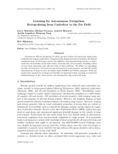
Figure 7: Single scan data in figures (a) and (b) of a walkway with leaves. In (a) the height difference of each scan point towards the average of neighboring points is shown. In (b) the result of the moving average filter with some leaves outliers. In (c) consecutive scans of a walkway after terrain classification are shown. leaves, leaf outlier rejection was not necessary for traversable surface extraction. Figure 8 presents results of traversable surface extraction in tests in our university campus. The detected traversable surfaces are presented in light gray, leaves and obstacles are represented in dark shades. Four different areas with different surfaces are presented: in Figure 8(a) a narrow pass by a waterway, water is not detected by the sensor. Figure 8(b) shows a narrow passage between bicycles; Figure 8(c) corresponds to a graveled drivable surface, stones and irregularities make the robot jump; and Figure 8(d) shows a walkway covered by leaves and bordered by a street road. 4.2
Landmark Extraction
The landmark extraction process was run off-line for landmark map building and on-line during robot navigation for position correction. The process is explained next: First traversable
ay rw te Wa
(a)
Narrow pass
Parked Bicycles
Leaves (d)
Street
(c)
Non-Traversable)
Walkway
Graveled terrain
Traversable
(b) Outlier (Traversable)
Figure 8: Traversable surface extraction during tests in the university campus. road classification of Section 4.1 was applied to scan data k to the last k − i scans where i = 200 which is equivalent to 5 seconds of stored scan data from the ring buffer explained in Section 3.2.1 (Figures 9(a)). After extracting and clustering traversable (flat) surface points, the edges of each side of the road were computed (Figure 9(b)). Then, least square line fitting based on eigenvectors (Duda and Hart, 1973) was applied to the set of edge points of 2 each side of the road. If the smallest eigenvalue of the covariance matrix (σzρ , Section 5.0.2) k which corresponds to the variance of the edge point distribution is smaller than a threshold 2 σzρ ≤ Tl (Tl had a predetermined value of 0.15 m), then the fitted straight line segment is k computed and it is determined that a landmark has been found (Figures 9(c) and 9(d)). By using not only the latest scan data but the past i scans it is possible to extract the landmarks even with partial occlusion of some parts of the road curbs. The landmarks are rotated and translated in global coordinates according to the actual pose of the robot. The selection of threshold Tl is not a trivial task; the threshold determines the variance of the distributed points. Landmarks were extracted only if the vehicle had a velocity over 0.25 m/sec and if it travelled a distance of 0.3 m. 4.3
Map Building
A map in Japanese Geodetic Datum 2000 (JGD 2000) Cartesian plane region IX (Geographical, 2008) coordinate system was built in advance with data taken with the robot operated with a joystick. The map contains landmarks and a global path which the robot must follow. The map was built off-line using a Kalman smoother approach. In this approach, the robot
curbstone
Left point cluster
road Scan at t Scan at t-1 Scan at t-3
σzρk
Right point cluster
σzρk
Scan at t-i
a
Last i scan data
b
Selected points after road detection
c
Least square method for straight line extraction
d
Left and right line landmarks extracted in global coordinates
Figure 9: Line landmark extraction process. trajectory is computed by dead reckoning (time stamped each sampling time t) with an initial position and covariance given by a DGPS measurement at time k − 1, then, dead reckoning and its covariance is propagated until a DGPS measurement at a time k is available. Dead reckoning is back propagated this time with initial position and covariance from DGPS data at time k to time k − 1. Finally the two position estimations with its covariances at the same epoch are used to compute the most likely robot trajectory. A detailed description of the method can be found in (Ohno et al., 2004b). Only DGPS data with HDOP ≤ 4 and number of satellites in view ≥ 5 satellites in view for the measurement was used (such DGPS information is considered reliable and was only available in open sky areas (Morales and Tsubouchi, 2007)). The T-URG was used for road extraction and line landmarks were extracted as described in Section 4.2 and added to the map. A set of 60 waypoints connected with straight lines were placed through the global path. During navigation the robot had to follow the waypoints until the goal. To check the consistency of the map, it was compared with RTK-GPS stand-still measurements (measurements in RTK mode can be done even close to trees if time for initialization is taken). The waypoints are shown in Figure 10 with cross points, RTK-GPS measured points are shown in asterisks, line landmarks are shown in dashed lines and detected flat surface is shown in light colored lines.
5
Vehicle Localization
Localization presents a difficult task because of dynamic and cluttered conditions in outdoor environments. There were trees, plants and bushes alongside the walkway which changed its characteristics according to the different seasons of the year. For localization, the use of trees as landmarks have already being proposed for example in (Guivant et al., 2002) and (Jutila et al., 2007). In the later a height of 1.3 m was selected as scanning height for tree extraction. In (Miettinen et al., 2007) SLAM for forest harvesters use tree trunks used as features, it is mentioned that tree trunk in dense forests is difficult if not impossible. In (Forsman and Halme, 2005) mapping of vast environments with trees is treated where tree trunks are modeled as cylinders. We considered the use of trunks as landmarks for localization using a sensor tilted upwards, however, we discarded it because the presence of people would considerably increase the complexity of tree trunk extraction. As seen in some images of Figure 1 the height of people and tree trunks (under the branches) is basically the same. The pictures were taken during Autumn, though, in Summer tree foliage is considerably thicker. The only structured part of the walkway was the road itself, so we decided to use it for
road RTK-DGPS Points Waypoints Line Landmark 8315
8600 8225
8310
8500 8220
8400 8305 8215
8200 8295
8100 8000
Y (South - North) in m
8300 8300
8210
7800
7790
8115
7900 7780 8110
7800 7770
8105
7700 7760
8100
7600 25500
25650
25800
25950
26100
7750
X (West - East) in m
Figure 10: Off-line created map in JGD 2000 Cartesian plane region IX coordinate system with a Kalman smoother approach. The map contains landmarks, waypoints and the extracted road. RTK-GPS ground truth measured points are shown to show the map consistency.
localization purposes using road limits as landmarks. The problems of this approach would be occlusion caused because of people around the robot. GPS when available provides global positioning, however close to buildings and trees there are measurement blackouts caused by GPS satellite signal blockage and in occasions when measurements are available, the position may be corrupted (jumps of several meters) caused by multipath effects. In our approach an EKF is used for robot pose estimation. The Kalman filter is a known technique well documented (Kalman, 1960), (Maybeck, 1979), (Leonard and Durrant-Whyte, 1992), (Y Bar-Shalom and Kirubarajan, 2001) (Thrun et al., 2005) that has been widely used in robotic applications. If the initial pose (x and y position and θ heading) are shown in advance and enough observations (landmarks and GPS in our case) are provided, the EKF can correct dead reckoning errors and track a single hypothesis of the vehicle pose. Robot localization is done towards the map built in global coordinates of Section 4.3. The EKF use low computational power compared with multiple hypothesis approaches like in (Fox, 1999) which offer the advantages of recovering from loosing track of the pose and getting lost but use high computational power. The robot pose is defined by a 3 dimensional state vector x = [x, y, θ]T . We modeled the robot as a common differential drive vehicle. Dead reckoning is computed with an approach similar to Gyrodometry presented by (Borenstein and Feng, 1996) with the difference that angular
velocity wk is computed using only information from a gyro of the IMU. This approach offers better precision than odometry because the different wheel size and tread caused by different air pressure in the tires and slippage (which commonly occurs in outdoor environments) does not affect the angular velocity measurement. Vehicle tangential velocity is calculated taking the average from left and right wheel tangential velocities which still suffers from the mentioned faults. Our dead reckoning in the worst of the cases presents an error of within 5% of the travelled distance. The update step of the Kalman filter is given by GPS and landmark matching corrections. These corrections update the predicted state of the filter in different sample times and are independent of each other. A normalized squared innovation test (or chi square test) was used as threshold for observations outlier rejection. If the value of χ2 is inside 95% confidence level then measurement update is performed, if not the observation is discarded (Y Bar-Shalom and Kirubarajan, 2001). The general scheme of vehicle localization is shown in Figure 11. GPS Data when ZGPSk available Motor Encoders
IMU
vk
EKF Prediction
ωk
Dead Pk-1 Reckoning
Line Landmark Detection ZLk
when available
NIS (chi square) Consistency Test
xk-1
EKF Correction
xk Pk
Figure 11: Vehicle localization framework.
5.0.1
GPS Based Localization Correction
The GPS receiver operated in StarFire DGPS mode ( Wide Area Differential GPS ) the correction signal comes from a Geostationary satellite without the necessity of having a base station close to the GPS receiver. GPS receivers have already a built in filter and outputs position measurements and statistics of such measurements in NMEA 2 sentence text protocol format. In this loosely coupled configuration, GGA NMEA sentence contains latitude and longitude global position and fix data, which after coordinate conversion to a Cartesian plane yields position in meters. GST (pseudo range noise statistics) sentence gives standard deviation of semi-major and semi-minor axis and angle of orientation of the covariance ellipse which, after coordinate conversion, gives the observation covariance matrix. A similar system using odometry and GPS for autonomous navigation is presented in (Ohno et al., 2004a), a more detailed explanation of the approach used in this work is presented in (Morales et al., 2008). A noise pre-filter proposed in (Huang and Tan, 2006) was applied for decreasing non-Gaussian noise in GPS measurements. The availability of GPS allows the system to localize itself in a global framework. 2
NMEA are the National Marine Electronics Association specifications for GPS output text format
5.0.2
Landmark Based Localization Correction
Landmarks constructed from the road limits were used for vehicle position correction. The approach explained in Subsection 4.2 was used for on-line landmark extraction during navigation. Using a road map to correct position during GPS blackouts is not a new issue and has been presented in works like (Najjar and Bonnifait, 2005) and (Levinson et al., 2007). The former uses the road centerline to correct the vehicle position, the later uses reflectivity data of a laser sensor towards the road lines to obtain sub-meter precision. In this work we used the road edges as landmarks to correct vehicle position. For line landmark observation models see (Arras and Siegwart, 1997) and (Siegwart and Nourbakhsh, 2004). The landmark correspondence between line segments in the map and the line segments which were extracted online was made using the left and right closest landmarks to the online extracted landmarks according to the actual pose of the robot. The data association problem is not complicated due to two factors: the assumption that the robot is always in the road and the nature of landmarks which were extracted from road edges where everything else is cluttered. Landmark observations correct vehicle’s position and orientation. Landmarks correction computation was done in global coordinates.
6
Navigation Approach
The general navigation approach is illustrated in Figure 12 and is detailed in the following subsections. Global planning
Obstacle Avoidance
MAP
global path
Landmark matching Dead reckoning GPS Localization
Localization
Navigation position
free space
Local Obstacle Map
Traversable surface extraction Obstacle detection
Figure 12: Navigation approach illustration. Vehicle localization for map based navigation following a pre-defined global path and traversable surface extraction and obstacle detection (non-traversable surface) for obstacle avoidance.
6.1
Global Path
A total of 60 waypoints linked by straight lines which connect the start and goal points were given to the robot in advance on the map described in Section 4.3. The waypoints were created to be on the left half side of the road because even though there are no traffic rules for pedestrians in walkways, in Japan the traffic is usually on the left side. When vehicle localization is accurate (Section 5) and no obstacles are detected the robot navigates consecutively passing through each waypoint. Therefore, the robot relies on accurate position
to navigate properly through the line segments among the waypoints (left side of Figure 12). A reliable collision avoidance sequence is necessary in the case there are obstacles between consecutive waypoints. The collision avoidance approach is explained below. 6.2
Collision Avoidance
Local obstacle avoidance was necessary to avoid routing out of the path because of localization errors (after blackout periods of DGPS and landmarks) and to handle people, bicycles and obstacles that appeared during the course. Many local collision avoidance methods have been previously developed. Potential field methods (Khatib, 1986) which sum attractive and repulsive forces from remote and close obstacles to determine the robot heading have low computational cost. The problem of such approaches is that they are unstable in narrow spaces (Koren and Borenstein, 1991). The Vector Field Histogram (VFH) method proposed in (Borenstein et al., 1991) can handle narrow openings, however it does not take into consideration vehicle dynamics for motion planning. Other methods such as the Curvature-Velocity Method (Simmons, 1996) and the Dynamic Window Approach (Fox et al., 1997) and its variations (Fox et al., 1998a), (Brock and Khatib, 1999) take into consideration the dynamics of the robot and control the robot in the domain of velocities. In this work a straightforward approach for obstacle avoidance was implemented. The method is similar to the Vector Field Histogram in the sense that it has free space regions built locally each sampling interval. There are two main differences: First, our approach also take past mapped data into consideration represented in point clouds. Therefore no confidence grid representation was used; the laser sensors used in this work, even if not noise-free, proved to be reliable enough to consider scanning data as certain values. During experimentation we did not experienced sensor mis-readings that would make the robot avoid non-existent obstacles. Second, motion planning takes into consideration the robot velocities. The approach is explained below. As the robot runs to the next goal waypoint it uses laser sensor data stored in the SSM (last 5 seconds, Section 3.2.1) mapped locally and total of thirteen free space sections (cuboids) were created each 10 deg every sampling time (the cuboids can be seen as free space histograms as in the VFH). Each free space cuboid represents a possible path the robot can travel to arrive to the next waypoint. The dimensions of the free spaces are: 4.0x0.7x2.0 m (LxWxH). Each cuboid was numbered from 1 to 13, giving the highest priority (“1”) to the space that change the robot heading the least with respect to the actual trajectory (Figure 13 shows the mapping of the free space cuboids). Additionally we give higher priority to cuboids on the left since the left circulation rule in Japan. In our approach, planning from actual robot position to the next waypoint uses a free space assumption (Koenig and Smirnov, 1997) in the sense that it assumes that there are no obstacles unless sensor readings prove otherwise. When an obstacle is detected, highest priority empty space cuboid is checked, if free, a line command from the actual position of the robot to the free space is sent to the motion control process (Section 3.2.2) and line following is executed resulting in the robot running through the empty space. If the space is not free, then next higher priority cuboid is checked and this process is repeated until there is an empty space found. If there is no free space, robot stops until a free path is available. Motion planning for line following commands developed in (Iida and Yuta, 1991) consider the actual displacement and heading of the robot to the desired line and adjust translational and rotational velocities to run on the desired line. Figure 14
12
Free space regions
10
Desired followed path
8 6 4 2 1 3 Robot Position
Way Point
5 7 9 11 13
Figure 13: Thirteen free space cuboids numbered in priority order. The dimensions of the free spaces are: 4.0x0.7x2.0 m (LxWxH).
illustrates the obstacle avoidance approach. When the robot is navigating towards the next waypoint (Figure 14 (a)) detects an obstacle in its trajectory (Figure 14 (b)). Free space cuboids are checked in priority order, when a free space is found, the robot runs through the free space (Figure 14 (c)). The process is repeated until no obstacle is found between the robot and the next waypoint; then the robot keeps running directly to the next waypoint (Figure 14(d)). The robot velocity was reduced according to the closeness of the detected obstacles. The robot maximum velocity was 0.8 m/sec when obstacles were further than 4 m and it stopped for 5 seconds when obstacles were detected closer than 0.12 m. Figure 15 depicts free space cuboids with real scan data mapped locally where an obstacle is detected in the right side cuboid (for view purposes, only three of the cuboids are illustrated). Vehicle accurate localization in outdoor environments is a difficult task. During long periods without any landmark detection nor GPS data, localization based on dead reckoning slowly degrades. In this case, robot tends to go out of the course (on narrow passages of the road, 1 m position error caused robot to go out of the road). In our approach, the developed flat surface extraction was robust enough to detect non-road areas as obstacles. Then obstacle avoidance is performed and the robot keeps moving within the road. Thus the robot keeps running on the road performing obstacle avoidance until the vehicle position is corrected by a landmark or a GPS measurement. The obstacle avoidance approach presented here as other local avoidance approaches, does not produce optimal solutions and can be trapped the local minima (u-shaped objects). When the robot is completely surrounded by obstacles and no free space is available, the robot stops and indefinitely keeps searching for a free space. As the robot has no rear ranging sensor, backward function was not implemented.
a
Obstacle
Way Point
Line to be followed
b
Line to be followed
c
Returning to path
d
Way Point
Figure 14: Free space created.
Figure 15: Free space cuboids (obstacle detected on the right side).
7
Experimental Results
In this section, preliminary results in our University campus, during the TC 2007 trials and final results during the TC 2007 final are presented.
7.1
Experimental Tests in University Campus
We performed preliminary experimental tests in three different paths in our university campus. Figure 16 shows the paths. Path 1 is a path between buildings and parking area for bicycles with a lenght of 337 m. Path 2 has mainly open sky areas with a length of 283 m. Path 3 is a road with up and down hills which has areas covered by tree canopy with a lenght of 313 m; for path 3 experiments were performed round trip with a total lenght of 626 m. During these experiments the robot was only provided with the waypoints it had to follow, thus no landmark correction was done. Localization was based in dead reckoning and DGPS (when available) and road detection kept the robot within the path limits. Localization results of path 3 are detailed in previous work (Morales et al., 2008). The performance of navigation performance is shown in table 1. The experimental results of this section were Table 1: Autonomous Navigation Experimental Results in University Campus. Robot autonomous navigation was tested in three different paths with different characteristics (road width, up and down hills, trees and buildings) Experimental Path Number of Trials Failed Runs Success Rate (%) Path 1 7 2 71.4 Path 2 10 0 100 Path 3 10 0 100 done during spring and summer, therefore there were no issues regarding fallen leaves. The reason the robot failed twice in path 1 was because there was no landmark map given to the robot to correct its position during GPS blackouts and the road did not have defined limits to keep the robot in path after road detection, then the robot got trapped in the bicycle parking lot facing an u-shaped obstacle. We consider that if the robot had a landmark map it would not have problem to run the path. For paths 2 and 3 as the road was well defined, even with some position error it could run to the end. Our approach proved to be robust towards pedestrian paths with defined limits. 7.2
Running the TC 2007 Trials
During trials in the target environment, obstacle avoidance algorithm was tested meticulously to prevent any malfunctioning that could cause a collision. Pedestrians and bicycle riders proved more natural and even more close to the robot during trials than in the challenge final itself when there were crowds of spectators group at sides of the road. During the trials, reliable DGPS data could be used in open sky areas (see Table 2). Furthermore, line landmarks could be extracted continuously because the laser sensors were not totally occluded by crowds of people. During trials, obstacle avoidance tests and several testing of robot navigation with pedestrians and bicycles passing by were performed. Snapshots taken during trial tests are shown in Figure 17. Figure 18 presents velocity of the robot running the TC2007 course route during a trial. During obstacle negotiation the robot will decrease its velocity according to the available free space cuboids (as was explained for Figure 15). In Figure 18 some scenes when the
Experimental Path in University Campus 13000
Waypoints Course
12900
Y South-North in m
Path 2
Path 3
12800
Path 3
12700
Path 2
12600 Path 1
Path 1 12500
Bicycle Parking Lot
12400 23800 a) In Google Maps
23900 24000 24100 X West-East in m b) Path used in Navigation
c) Path Characteristics
Figure 16: Free space cuboids (obstacle detected on the right side).
Figure 17: Autonomous running snapshots during trials. robot decreased its velocity are also shown: Figure 18(a) shows the robot as it decreased its speed in order to go around the person standing in the middle of the road; in Figure 18(b) the robot reduced its speed to about 0.5 m/s to avoid the corner of a small wall; in Figure 18(c) the robot avoided collision with a corner of a bridge; finally in Figure 18(d) the robot avoided jumping over a road curbstone. In the case of Figure 18(a), the person on the left of the robot becomes an obstacle, there is only free space on the right so the robot follows it successfully going around the person and continue towards the next waypoint. After extensive autonomous running tests, our robot achieved autonomous navigation of the 1 km course within the path several times without collisions. The total number of landmark and GPS corrections during two of the trials are presented in Table 2. Figure 21 shows standard deviation (2σ) vs time results. 7.3
Running the TC 2007 Final
On the challenge final, large number of people between spectators, organizers and media were present especially around the start line. Figure 19 presents some snapshots of our robot while running the Challenge final. In all stages the robot was accompanied by team members and TC 2007 officers as seen in all the pictures. The course included bridge sections
Free spaces
Speed (m/s)
(b)
(c)
Free spaces
1 0.9 0.8 0.7 0.6 0.5 0.4 0.3 0.2 0.1 0 -0.1 0
2
4
(a)
6
8
Free space
10
12 14 Time (mins)
16
18
20
(d)
22
24
Free space
Figure 18: Speed vs time during trials on November 16th 2007. and narrow paths which had roadside trees, fallen leaves and people especially at start and goal points. Spectators, TC 2007 officers and camera men entered several times in the laser sensor scan area (as depicted in several of the pictures). Despite partial occlusion of road edges, straight segment landmarks for robot position correction could be extracted using the tilted laser scanners. Ultimately, landmark matching and collision avoidance played the biggest role during autonomous navigation of the TC 2007 final. Table 2 presents the amount of corrections in two trials and final run of the TC. During the trials DGPS worked was used in open sky areas where more than 60% of the measurements passed the consistency check to correct vehicle position. DGPS corrections during the TC2007 final were almost non existent, in fact only in one open sky area NIS accepted correction was available. Our robot was able to run to the goal without any collision at an average velocity of 0.72 m/s. Because of accumulated position error, robot stopped within 0.80 m of the goal line though it was determined by challenge organizers that robots stopping within 10 m of the goal had
Figure 19: Autonomous running snapshots during the challenge final. Table 2: Total of landmark and DGPS corrections during 1km autonomous navigation. Experiment Landmark DGPS Corrections Date Corrections NIS Accepted NIS Rejected November 16th Trial Run 1334 99 58 November 17th TC Final Run 1412 1 37 th November 17 TC Exhibition Run 1338 113 24 completed the challenge. This was because even if robot could correct its position laterally with landmarks, it could not correct global position with DGPS. Figure 20 shows estimated robot trajectory and the different navigation modes during TC 2007 final autonomous run where no one DGPS correction was incorporated for position error correction. Figure 21 shows the time vs positioning error graph for 1 km navigation during trial on November 16th (light colored), during the TC2007 final (in dark) and during an exhibition run after TC2007 final (dashed), the double of the square root of the semi-major axis of the covariance ellipse (2σ) values are shown. According to the values presented in Table 2, DGPS corrections during the TC2007 final were almost non existent, in fact only in one open sky area NIS accepted correction was available. For the trial and the exhibition runs a relative large number of accepted corrections were available. Given this difference in DGPS corrections, positioning during the final relied heavily on line-landmark based corrections. Figure 22 presents results of traversable surface extraction during the TC2007 finals. The complete set of laser scan data corresponding to road surface, curbs, leaves and small obstacles is shown in the figure, the detected traversable surface is presented in light gray and leaves and other objects are represented in dark shades. Four areas with different surfaces were selected: in Figure 22(a) a crowded section of the road, Figure 22(b) a narrow passage over a bridge, Figure 22(c) corresponds to a rather rough surface and Figure 22(d) the end section of the course heavily covered by leaves. During the TC2007 final several of the obstacles for the robot navigation were the large number of spectators who would stand very close to the path and even in from of the robot. Figure 23 shows the velocity vs time graph for the final. As already presented in sections 3.1 and 3.2, the implemented system runs entirely in a single
Autonomous Running Log 8600
Dead Reckoning Line landmark Avoidance GPS
8500 8400
Y (South - North) in m
8300 8200 8100 8000 7900 7800 7700 7600 25500
25650 25800 25950 X (West - East) in m
26100
Figure 20: Robot Trajectory Computed During Autonomous Running in the TC 2007 Final. Position correction performed with landmarks are shown in darker 1 points and position correction by GPS are depicted in asterisk points. Positions where obstacle avoidance was performed are shown in light points. Lighter points refer to positions where neither position correction nor obstacle avoidance was performed, thus, only dead reckoning computed robot position. Overlapping is also present.
Standard Deviation 2σ (m)
3.5
Trial 11-16 Final 11-17 Exhibition 11-17
No corrections available
3 2.5 2 1.5 1
DGPS corrections (in open sky areas)
DGPS corrections (in open sky areas)
0.5 0 0
2
4
6
8
10 12 Time (mins)
14
16
18
20
22
Figure 21: Positioning error for 1 km navigation during trials and final.
(b) Paved road in bridge section
(c) Tiled road Traversable Outlier (Traversable) Non-Traversable)
(d) Paved narrow road
(a) Paved road surrounded by trees
Speed (m/s)
Figure 22: Traversable surface extraction results during TC2007 final on November 17th 2007.
1 0.9 0.8 0.7 0.6 0.5 0.4 0.3 0.2 0.1 0 -0.1
Velocity
0
2
4
6
8
10
12
14
16
18
20
22
Time (mins)
Figure 23: Speed vs time during TC2007 final on November 17th 2007.
notebook computer. One merit of the implemented system is its simplicity, and the authors consider this as an important factor for completing the TC2007 challenge. Most of the processes were CPU intensive, demanding large amounts of memory to store/retrieve sensor data and high I/O transfer in USB interfaces. Figure 24 shows the system performance measurements while running the TC2007 final; the average CPU usage was 43% (Figure 24(a)) while memory usage was 98% of the total system memory with very little need for swap memory (Figure 24(b)).
70 % used CPU
60
system user
50 40 30 20 10 0 2
4
6
8
10
12
14
16
18
20
22
Time (mins)
(a)
Resource used (MB)
1010
Memory Swap
1000 990 980 970 50 40 30 20 10 0 2
4
6
8
10
12
14
16
18
20
22
Time (mins)
(b)
Figure 24: System performance indicators during TC2007 final on November 17th 2007.
8
Discussion and Lessons Learned
In this section, the authors present a summary of the experiences gained during the TC 2007. • System typical failures: -A typical failure in our localization approach could happen in the case that DGPS is not available in long road sections without defined edges, therefore, landmarks would not be extracted and the robot could loose its way; since EKF is a single hypothesis approach it can not recover from getting lost, unless the filter is reset, but our system did not have that functionality. However, the traversable surface extractor kept the robot in track. -In locations where too many fallen leaves were present, the height between the road and non road is basically the same, therefore our road classifier would classify everything as traversable. -Traversable surface extraction was implemented to work in nearly flat surfaces and gentle slopes, and is robust even in rough terrain. However in its current form, steep slopes will be detected as obstacles. -Obstacle avoidance would be trapped in the local minima towards u-shaped
objects or people surrounding the robot. - A problem we were facing regarding the motion control system is that it had overshooting when following a selected line, sometimes not being able to avoid obstacles or course outs (which we regarded at first as a perception problem). Once the robot parameters were tuned, our robot was able to smoothly run the walkways. • Regarding fallen leaves, one problem we observed during experimentation was that in windy days (which only happened one time), leaves were blown up all over the place. In our approach if such leaves are detected by the laser, then they would be classified as non-traversable points (obstacles) and the robot would try to avoid non existent obstacles. • The final conditions of the environment were impossible to predict. We could not know if there were going to be large amounts of people around the robot or it would generate less interest and be a more natural run. In the event final there were crowds of people around the robot through the first 120 m, then the amount of people decreased through the course, however, close to the goal line, there were again a large amount of people waiting for the robots to arrive. During the event, people were aware that robots were passing and stood at the edges of the road. In the end, real world conditions for robot navigation were present during the trials where pedestrians and bicycles were naturally passing and not during the TC final where people were expecting the robots. • We had a couple of issues regarding DGPS: First, we had a problem when the TURG was used together with the beacon DGPS; the signal to noise ratio of the beacon receiver (even if isolated) was too low to receive correction signals from the Japanese coast guard. Therefore we could not use the beacon and instead we used StarFire DGPS (Hatch and Sharpe, 2004) which is only available in open sky areas. DGPS using a beacon receiver offer the best solution (measurement availability and reliability) in woodland environments (Morales and Tsubouchi, 2007). The second issue was during the TC 2007 final, before the run started, our robot was placed under tree canopy for around 30 minutes, therefore the GPS receiver had to be initialized under the trees. We have empirically tested that if GPS is not initialized in open sky the amount of available data when the GPS receiver re-enters tree canopy is much more less than if it is initialized in open sky. This was the only case where we had such a problem with the GPS, in all our other autonomous tests the GPS was initialized in open sky. • During trials we found that the most curious people were the elder and children, who after asking if the robot could detect and avoid them, stood in front of it to see its evasive action. Unfortunately during this event none of the robots had people interactive components. We consider that a future version of our robot should have some kind of interactive component.
9
Conclusions
In this paper a self-contained mobile robot for autonomous navigation in outdoor concurred pedestrian walkways was described. The robot main characteristics are its simplicity in
hardware and software. All the computation was performed on board in a single off the shelf laptop. The difficulties of navigation in outdoor transited paths mostly covered by trees as well as our system integration approach were also reported. For localization a multisensor approach using an EKF for data fusion of wheel encoders, IMU, GPS and laser scanner sensors was implemented. In addition, an effective method for road detection containing considerable amounts of fallen leaves was proposed. When estimated position was not precise enough, extraction of the traversable and non-traversable (obstacles) road for obstacle avoidance kept the robot in track. Keeping the priority of pedestrian integrity, our robot system was able to run in public pedestrian walkways (TC 2007 course) successfully multiple times. We consider that robust navigation was achieved because of the complementary functionality of the proposed system. Movies and snapshots of our robot are shown in (Okugaigumi, 2007). In this work, when the robot detected an obstacle, it was not able to perform object recognition to distinguish between an human, bicycle, tree or other robot. As future research, object detection and recognition is necessary for proper decision making on path planning. Moreover, authors plan to keep researching in human-robot and robot-robot interactions and traffic decisions. Lately, the use of camera in outdoor environments has proved to be a robust method for vehicle localization, we think that camera-laser scanner is a appropriate configuration for robust outdoor navigation. Finally, as future work, we plan to add terrain roughness classification by IMU’s vertical axis accelerometer to the map. Roughness information would allow to correct or reset robot’s position according to the terrain surface change. Acknowledgements The authors acknowledge TC 2007 organizers, the government of the city of Tsukuba as well as its habitants for the support and realization of the event. Authors also thank Hokuyo Automatic Co., Ltd. for providing T-URG laser scanner sensor and GNSS Technologies Inc. for their technical support on GPS. Finally the authors would like to thank W. Tokunaga, H. Kuniyoshi, A. Hirosawa, Y. Nagasaka and Y. Suzuki for their help during experimentation. References AAAI (2008). Association for the Advancement of Artificial Intelligence (AAAI) [www page]. Retrieved December 2, 2008 from http://www.aaai.org. Arras, K. O. and Siegwart, Y. (1997). Feature extraction and scene interpretation for mapbased navigation and map building. In Proc. of SPIE, Mobile Robotics XII, pages 42–53. Bacha, A., Bauman, C., Faruque, R., Fleming, M., Terwelp, C., Reinholtz, C., Hong, D., Wicks, A., Alberi, T., Anderson, D., , Cacciola, S., Currier, P., , Dalton, A., Farmer, J., Hurdus, J., Kimmel, S., King, P., Taylor, A., Covern, D. V., and Webster, M. (2008). Team VictorTango’s entry in the DARPA Urban Challenge. Journal of Field Robotics Special Issue on the 2007 DARPA Urban Challenge, Part I, 25(1):467–492. Bajracharya, M., Howard, A., Matthies, L., Tang, B., and Turmon, M. (2009). Autonomous
off-road navigation with end-to-end learning for the lagr program. Journal of Field Robotics, 26(1):3–25. Balch, T. and Yanco, H. A. (2002). Ten years of the aaai mobile robot competition and exhibition: looking back and to the future. AI Magazine, 23(1):13–22. Bohren, J., Foote, T., Keller, J., Kushleyev, A., Lee, D., Stewart, A., Vernaza, P., Derenick, J., Spletzer, J., and Satterfield, B. (2008). The Ben Franklin Racing Team’s entry in the 2007 DARPA Urban Challenge. Journal of Field Robotics Special Issue on the 2007 DARPA Urban Challenge, Part II, 25(1):598–614. Borenstein, J. and Feng, L. (1996). Gyrodometry: a new method for combining data from gyros and odometry in mobile robots. In In Proceedings of the 1996 IEEE International Conference onRobotics and Automation, pages 423–428. Borenstein, J., Koren, Y., and Member, S. (1991). The vector field histogram - fast obstacle avoidance for mobile robots. IEEE Journal of Robotics and Automation, 7:278–288. Brock, O. and Khatib, O. (1999). High-speed navigation using the global dynamic window approach. In Proc. of the 1999 IEEE Int. Conf. on Robotics and Automation, pages 341–346. Buhmann, J., Burgard, W., Cremers, A., Fox, D., Hofmann, T., Schneider, F., Strikos, J., and Thrun, S. (1995). The mobile robot Rhino. AI Magazine, 16(1). Burgard, W., Cremers, A. B., Fox, D., Hahnel, D., Lakemeyer, G., Schulz, D., and Steiner, W. (1999). Experiences with an interactive museum tour-guide robot. Artificial Intelligence, 114:1–2. DARPA (2008). Darpa Urban Challenge [www page]. Retrieved December 2, 2008 from http://www.darpa.mil/grandchallenge/index.asp. Duda, R. O. and Hart, P. E. (1973). Pattern Classification and Scene Analysis. John Wiley and Sons. Forsman, P. and Halme, A. (2005). 3-d mapping of natural environments with trees by means of mobile perception. IEEE Transactions on Robotics, 21(3):482–490. Fox, D. (1999). Markov localization for mobile robots in dynamic environments. Journal of Artificial Intelligence Research, 11:391–427. Fox, D., Burgard, W., and Thrun, S. andCremers, A. (1998a). A hybrid collision avoidance method for mobile robots. In Proc. of the 1998 IEEE International Conference on Robotics and Automation, pages 1238–1243. Fox, D., Burgard, W., and Thrun, S. (1997). The dynamic window approach to collision avoidance. IEEE Robotics and Automation Magazine, 4(1):23 – 33. Fox, D., Burgard, W., Thrun, S., and Cremers, A. (1998b). Position estimation for mobile robots in dynamic environments. In Proc. of the National Conference on Artificial Intelligence. Geographical (2008). Geographical survey institute government of japan [www page]. Retrieved August 2, 2008 from http://vldb.gsi.go.jp/sokuchi/surveycalc/. Google (2008). Google Lunar X PRIZE [www page]. Retrieved December, 2008 from http: //www.googlelunarxprize.org/.
Guivant, J., Masson, F., and Nebot, E. (2002). Simultaneous localization and map building using natural features and absolute information. Robotics and Autonomous Systems, 40:79–90(12). Guivant, J., Nebot, E., and Baiker, S. (2000). Autonomous navigation and map building using laser range sensors in outdoor applications. Journal of Robotic Systems, 17:3817– 3822. Hatch, R. and Sharpe, R. (2004). Recent improvements to the starfire global dgps navigation software. In Journal of Global Positioning Systems, volume 3, pages 143–153. Hiroaki, K., Minoru, A., Yasuo, K., Itsuki, N., Eiichi, O., and Hitoshi, M. (1998). Robocup: A challenge problem for ai and robotics. pages 1–19. Hokuyo (2008). Hokuyo automatic co., ltd. [www page]. Retrieved August 2, 2008 from http://www.hokuyo-aut.jp. Huang, J. and Tan, H. S. (2006). A low order dgps-based vehicle positioning system under urban environment. In IEEE/ASME Transactions on Mechatronics, volume 11, pages 567–575. Iida, S. and Yuta, S. (1991). Vehicle command system and trajectory control for autonomous mobile robots. In Proc. of the 1991 IEEE/RSJ International Conference on Intelligent Robots and Systems (IROS) International Workshop, pages 212–217. Jackel, L. D., Krotkov, E., Perschbacher, M., Pippine, J., and Sullivan, C. (2006). The darpa lagr program: Goals, challenges, methodology, and phase i results. Journal of Field Robotics, 23:945–973. Jutila, J., Kannas, K., and Visala, A. (2007). Tree measurement in forest by 2d laser scanning. In Proc. of the 2007 International Symposium on Computational Intelligence in Robotics and Automation, pages 491–496. Kalman, R. E. (1960). A new approach to linear filtering and prediction problems. Transaction of the ASME Journal of Basic Engineering, pages 35–45. Khatib, O. (1986). Real-time obstacle avoidance for manipulators and mobile robots. International Journal of Robotics Research, 5(1):90–98. Koenig, S. and Smirnov, Y. (1997). Sensor-based planning with the freespace assumption. In Proc. of the 1997 IEEE International Conference on Robotics and Automation, pages 3540–3545. Koren, Y. and Borenstein, J. (1991). Potential field methods and their inherent limitations for mobile robot navigation. In Proc. of the 1991 IEEE International Conference on Robotics and Automation, pages 1398–1404. Kortenkamp, D., Huber, M., Cohen, C., Raschke, U., Bidlack, C., Congdon, C. B., Koss, F., and Weym, T. (1993). Integrated mobile-robot design-winning the aaai 1992 robot competition. IEEE Expert: Intelligent Systems and Their Applications, 8(4):61–73. Leonard, J., How, J., Teller, S., Berger, M., Campbell, S., Fiore, G., Fletcher, L., Frazzoli, E., Huang, A., Karaman, S., Koch, O., Kuwata, Y., Moore, D., Olson, E., Peters, S., Teo, J., Truax, R., Walter, M., Barrett, D., Epstein, A., Maheloni, K., Moyer, K., Jones, T., Buckley, R., Antone, M., Galejs, R., Krishnamurthy, S., and Williams, J. (2008). A perception-driven autonomous urban vehicle. Journal of Field Robotics Special Issue on the 2007 DARPA Urban Challenge, Part III, 25(1):727–774.
Leonard, J. J. and Durrant-Whyte, H. F. (1992). Directed Sonar Sensing for Mobile Robot Navigation. Kluwer Academic Publishers, Norwell, MA, USA. Levinson, J., Montemerlo, M., and Thrun, S. (2007). Map-based precision vehicle localization in urban environments. In Proceedings of Robotics: Science and Systems. Liscano, R., Fayek, R. E., Manz, A., Stuck, E. R., and Tigli, J.-Y. (1995). Using a blackboard to integrate multiple activities and achieve strategic reasoning for mobile-robot navigation. IEEE Expert: Intelligent Systems and Their Applications, 10(2):24–36. Maybeck, P. S. (1979). Stochastic models, estimation, and control, volume 1 of Mathematics in Science and Engineering. Academic Press. Miettinen, M., Ohman, M., Visala, A., and Forsman, P. (2007). Simultaneous localization and mapping for forest harvesters. In Proc.of the 2007 IEEE International Conference on Robotics and Automation 2007, pages 517–522. Miller, I., Campbell, M., Huttenlocher, D., Kline, F.-R., Nathan, A., Lupashin, S., Catlin, J., Schimpf, B., Moran, P., Zych, N., Garcia, E., Kurdziel, M., and Fujishima, H. (2008). Team cornell’s skynet: Robust perception and planning in an urban environment. Journal of Field Robotics Special Issue on the 2007 DARPA Urban Challenge, Part I, 25(1):493–527. Miyai, T. and Yuta, S. (1997). Design and implementation of distributed controller and its operating system for autonomous mobile robot platform. In Proc. of the 1997 International Conference on Field and Service Robotics. Montemerlo, M., Becker, J., Bhat, S., Dahlkamp, H., Dolgov, D., Ettinger, S., Haehnel, D., Hilden, T., Hoffmann, G., Huhnke, B., Johnston, D., Klumpp, S., Langer, D., Levandowski, A., Levinson, J., Marcil, J., Orenstein, D., Paefgen, J., Penny, I., Petrovskaya, A., Pflueger, M., Stanek, G., Stavens, D., Vogt, A., and Thrun, S. (2008). Junior: The stanford entry in the Urban Challenge. Journal of Field Robotics Special Issue on the 2007 DARPA Urban Challenge, Part II, 25(1):569–597. Morales, Y., Takeuchi, E., and Tsubouchi, T. (2008). Vehicle localization in outdoor woodland environments with sensor fault detection. In Proc of the 2008 IEEE International Conference on Robotics and Automation, pages 449–454. Morales, Y. and Tsubouchi, T. (2007). Gps moving performance on open sky and forested paths. In Proc. of the 2007 IEEE/RSJ International Conference on Intelligent Robots and Systems, pages 3180–3185. Najjar, M. E. E. and Bonnifait, P. (2005). A road-matching method for precise vehicle localization using belief theory and kalman filtering. Autonomous Robots, 19(2):173– 191. Ohno, K., Tsubouchi, T., Shigematsu, B., and Yuta, S. (2004a). Differential gps and odometry-based outdoor navigation of a mobile robot. Advanced Robotics, 18(6):611–635. Ohno, K., Tsubouchi, T., and Yuta, S. (2004b). Outdoor map building based on odometry and rtk-gps positioning fusion. In Proc. of the 2004 IEEE International Conference on Robotics and Automation. ICRA 2004, pages 684–690, New Orleans. Okugaigumi (2007). Team okugaigumi movies and pictures [www page]. Retrieved August 2, 2008 from http://www.roboken.esys.tsukuba.ac.jp/~yoichi/tc2007.html.
PC-Yamabico (2008). Pc-yamabico project (sourceforge) [www page]. Retrieved December 2, 2008 from http://sourceforge.jp/projects/pc-ymbc/. Penn (2008). Penn state abington mini grand challenge [www page]. Retrieved December 2, 2008 from http://www.cede.psu.edu/users/avanzato/robots/contests/outdoor/ index.htm. Pradalier, C., Hermosillo, J., Koike, C., Braillon, C., Bessi`ere, P., and Laugier, C. (2005). The cycab: a car-like robot navigating autonomously and safely among pedestrians. Robotics and Autonomous Systems, 50(1):51–68. Rainwater, R. S., Arrick, R., and Brown, J. (2008). Robots.net [www page]. Retrieved December 2, 2008 from http://robots.net/. Robo-Magellan (2008). Seattle robotics society, robo-magellan [www page]. Retrieved December 2, 2008 from http://www.robothon.org/robothon/robo-magellan.php. Robocup (2008). Robocup [www page]. Retrieved December 2, 2008 from http://www. robocup.org/. Robotour (2008). Robotour 2008 [www page]. Retrieved December 2, 2008 from http: //robotika.cz/competitions/robotour2008/en. Siegwart, R. and Nourbakhsh, I. (2004). Introduction to Autonomous Mobile Robots. A Bradford Book, The MIT Press, Cambridge, Massachusetts, London, England. Simmons, R. (1996). The curvature-velocity method for local obstacle avoidance. In Proc. of the 1996 IEEE International Conference on Robotics and Automation (ICRA 1996), pages 3375–3382. Simmons, R., Goodwin, R., Haigh, K., Koenig, S., O’Sullivan, J., and Veloso, M. M. (1997). Xavier: Experience with a layered robot architecture. In ACM SIGART Intelligence magazine. Takeuchi, E. and Tsubouchi, T. (2003). Integration and synchronization of external sensor data for a mobile robot. In Proc. of 2003 SICE Annual Conference. Takeuchi, E. and Tsubouchi, T. (2006). Sensory data processing middlewares for service mobile robot applications. In Proc of the 2006 SICE-ICASE International Joint Conference. Thrun, S., Beetz, M., Bennewitz, M., Burgard, W., Creemers, A., Dellaert, F., Fox, D., Hahnel, D., Rosenberg, C., Roy, N., Schulte, J., and Schulz, D. (2000). Probabilistic algorithms and the interactive museum tour-guide robot minerva. International Journal of Robotics Research, 19(1):972–999. Thrun, S., Burgard, W., and Fox, D. (2005). Probabilistic Robotics (Intelligent Robotics and Autonomous Agents). The MIT Press. Thrun, S., Montemerlo, M., Dahlkamp, H., Stavens, D., Aron, A., Diebel, J., Fong, P., Gale, J., Halpenny, M., Hoffmann, G., Lau, K., Oakley, C., Palatucci, M., Pratt, V., Stang, P., Strohband, S., Dupont, C., Jendrossek, L.-E., Koelen, C., Markey, C., Rummel, C., van Niekerk, J., Jensen, E., Alessandrini, P., Bradski, G., Davies, B., Ettinger, S., Kaehler, A., Nefian, A., and Mahoney, P. (2006). Stanley: The robot that won the DARPA Grand Challenge. Journal of Field Robotics, 23(1):661–692.
Tsukuba, C. (2008). New technology foundation tsukuba challenge: Real world robot challenge [www page]. Retrieved August 2, 2008 from http://www.robomedia.org/ challenge (in Japanese). Urmson, C., Anhalt, J., Bae, H., Bagnell, J. D., Baker, C., Bittner, R. E., Brown, T., Clark, M. N., Darms, M., Demitrish, D., Dolan, J., Duggins, D., Ferguson, D., Galatali, T., Geyer, C. M., Gittleman, M., Harbaugh, S., Hebert, M., Howard, T., Kolski, S., Likhachev, M., Litkouhi, B., Kelly, A., McNaughton, M., Miller, N., Nickolaou, J., Peterson, K., Pilnick, B., Rajkumar, R., Rybski, P., Sadekar, V., Salesky, B., Seo, Y.W., Singh, S., Snider, J. M., Struble, J. C., Stentz, A. T., Taylor, M., Whittaker, W. R. L., Wolkowicki, Z., Zhang, W., and Ziglar, J. (2008). Autonomous driving in urban environments: Boss and the Urban Challenge. Journal of Field Robotics Special Issue on the 2007 DARPA Urban Challenge, Part I, 25(1):425–466. Urmson, C., Anhalt, J., Bartz, D., Clark, M., Galatali, T., Gutierrez, A., Harbaugh, S., Johnston, J., Kato, H., Koon, P. L., Messner, W., Miller, N., Mosher, A., Peterson, K., Ragusa, C., Ray, D., Smith, B. K., Snider, J. M., Spiker, S., Struble, J. C., Ziglar, J., and Whittaker, W. R. L. (2006). A robust approach to high-speed navigation for unrehearsed desert terrain. Journal of Field Robotics, 23(1):467–508. Wijesoma, W., Kodagoda, K., and Balasuriya, A. (2004). Road-boundary detection and tracking using ladar sensing. Robotics and Automation, IEEE Transactions on, 20(3):456–464. Wolf, D., Sukhatme, G., Fox, D., and Burgard, W. (2005). Autonomous terrain mapping and classification using hidden markov models. Proc. of the 2005 IEEE International Conference on Robotics and Automation, pages 2026–2031. Y Bar-Shalom, X. L. and Kirubarajan, T. (2001). Estimation with Applications ot Tracking and Navigation. Wiley-Interscience Publication. Yuta, S., Suzuki, S., and Iida, S. (1993). Implementation of a small size experimental selfcontained autonomous robot-sensors, vehicle control, and description of sensor based behavior. In The 2nd International Symposium on Experimental Robotics II, pages 344– 358, London, UK. Springer-Verlag.