theory, we know that if the discrete system ...... [5] T. I. Fossen, Guidance and Control of Ocean Vehicles. ... [7] W. L. Brogan, Modern Control Theory, 3rd ed.
TECHNICAL REPORT 1968 February 2008
Autonomous Underwater Vehicle Navigation P. A. Miller SSC San Diego J. Farrell Y. Zhao V. Djapic University of California, Riverside
Approved for public release; distribution is unlimited.
SSC San Diego
iv
TECHNICAL REPORT 1968 February 2008
Autonomous Underwater Vehicle Navigation P. A. Miller SSC San Diego J. Farrell Y. Zhao V. Djapic University of California, Riverside
Approved for public release; distribution is unlimited.
SSC San Diego San Diego, CA 92152-5001
SSC SAN DIEGO San Diego, California 92152-5001 M. T. Kohlheim, CAPT, USN Commanding Officer
C. A. Keeney Executive Director
ADMINISTRATIVE INFORMATION The work described in this report was performed for the Naval Explosive Ordnance Disposal Technology Division, Underwater Director Code 51B, by the Ocean Technology Branch (Code 56640) SPAWAR Systems Center San Diego (SSC San Diego) and the University of California, Riverside. Released by T. B. Augustus, Acting Head Ocean Technology Branch
Under authority of L. B. Collins, Head Ocean Systems Division
This is a work of the United Sates Government and therefore is not copyrighted. This work may be copied and disseminated without restriction. Many SSC San Diego public release documents are available in electronic format at http://www.spawar.navy.mil/sti/publications/pubs/index.html.
SB
CONTENTS 1 Introduction
1
1.1
System Description . . . . . . . . . . . . . . . . . . . . . . . . . . . . . . . . . . . . .
1
1.2
Notation . . . . . . . . . . . . . . . . . . . . . . . . . . . . . . . . . . . . . . . . . . .
2
2 Model Derivation
2
3 Navigation
4
3.1
Inertial Measurement Unit . . . . . . . . . . . . . . . . . . . . . . . . . . . . . . . . .
6
3.2
Augmented System Equations . . . . . . . . . . . . . . . . . . . . . . . . . . . . . . .
6
3.3
Mechanization Equations . . . . . . . . . . . . . . . . . . . . . . . . . . . . . . . . .
7
3.4
Error State Equations . . . . . . . . . . . . . . . . . . . . . . . . . . . . . . . . . . .
7
3.5
Time Propagation . . . . . . . . . . . . . . . . . . . . . . . . . . . . . . . . . . . . .
9
3.6
Measurement Corrections . . . . . . . . . . . . . . . . . . . . . . . . . . . . . . . . .
9
3.6.1
Attitude Update . . . . . . . . . . . . . . . . . . . . . . . . . . . . . . . . . . 10
3.6.2
Doppler Velocity Log Update . . . . . . . . . . . . . . . . . . . . . . . . . . . 11
3.6.3
Long Baseline Update . . . . . . . . . . . . . . . . . . . . . . . . . . . . . . . 12
3.6.4
Pressure Update . . . . . . . . . . . . . . . . . . . . . . . . . . . . . . . . . . 14
4 Analysis
15
4.1
Incremental LBL Dropouts, Limited Compass Aiding . . . . . . . . . . . . . . . . . . 17
4.2
Incremental DVL Beam Dropouts, No LBL Aiding . . . . . . . . . . . . . . . . . . . 19
5 Experimental Results
21
6 Future Work
23
7 References
24
iii
LIST OF FIGURES 1
Vehicle sensor configuration . . . . . . . . . . . . . . . . . . . . . . . . . . . . . . . .
2
Long baseline interrogation cycle . . . . . . . . . . . . . . . . . . . . . . . . . . . . . 13
3
North–East plot of incremental LBL dropout scenario . . . . . . . . . . . . . . . . . 16
4
East position error η˜1 (y) for incremental LBL dropout scenario . . . . . . . . . . . . 17
5
Azimuth error ρ(ψ) ˜ for incremental LBL dropout scenario . . . . . . . . . . . . . . . 18
6
Sound speed error c˜ for incremental LBL dropout scenario . . . . . . . . . . . . . . . 18
7 8
Velocity error ν˜1 (u) for incremental DVL dropout scenario . . . . . . . . . . . . . . . 19 Accelerometer bias error ˜ba (u) for incremental DVL dropout scenario . . . . . . . . . 20
9
North, east, and down position error δη1 standard deviation . . . . . . . . . . . . . . 21
10
Long baseline transponder 1 residual . . . . . . . . . . . . . . . . . . . . . . . . . . . 22
11
Sound speed estimate cˆ . . . . . . . . . . . . . . . . . . . . . . . . . . . . . . . . . . 23
12
Semi-log plots of azimuth and gyro bias error standard deviations . . . . . . . . . . . 24
13
Accelerometer and gyro bias estimates . . . . . . . . . . . . . . . . . . . . . . . . . . 25
14
Doppler velocity log beam 1 residual . . . . . . . . . . . . . . . . . . . . . . . . . . . 25
iv
2
EXECUTIVE SUMMARY This report considers the vehicle navigation problem for an autonomous underwater vehicle with six degrees of freedom. We approach this problem using an error state formulation of the Kalman filter. Integration of the vehicle’s high-rate inertial measurement unit’s accelerometers and gyros allow time propagation while other sensors provide measurement corrections. The low-rate aiding sensors include a Doppler velocity log, an acoustic long baseline system that provides round-trip travel times from known locations, a pressure sensor for aiding depth, and an attitude sensor. Measurements correct the filter independently as they arrive, and as such, the filter is not dependent on the arrival of any particular measurement. The navigation system can estimate critical bias parameters that improve performance. The result is a robust navigation system. Simulation and experimental results are provided.
1.
INTRODUCTION
With the emergence of inspection-class autonomous underwater vehicles, navigation and navigational accuracy are becoming increasingly important. Without an operator in the loop, the vehicle itself must use sensors to determine its location, orientation, and motion. Many of these unique sensors rely on acoustic measurements that present interesting challenges. The problem is how to effectively use all available sensor inputs to provide a continuous and robust estimate of the vehicle’s navigational state. One approach is to treat each sensor independently, each measuring a specific state. A position sensor measures position, a velocity sensor measures velocity, and so forth. This solution, however, is clearly not robust and does not take advantage of the kinematic relationships between states and measurements. Consider the situation where sensor performance degrades and measurement updates become sporadic. If position fixes are not regularly available, how should the position state evolve? One could dead-reckon with the velocity and heading, then blend this estimate with each position fix, but is this ad-hoc method optimal? Here, we present an approach using an error state formulation of the Kalman filter to provide an optimal and robust solution to the vehicle navigation problem. This report concentrates on the application of the Kalman filter and development of the model and filter algorithms. It does not attempt to justify the Kalman filter [1, 2, 3] or make comparisons to other algorithms. This report is an extension of previous work [4]. Here, we expand upon our approach and analysis, and reformulate algorithms to provide a more theoretically concrete implementation. The following section describes the system of interest. Section 2 develops the continuous-time model for this system, while Section 3 formulates the corresponding navigation equations. In Section 4, we choose several interesting scenarios to analyze critical aspects of our approach. The final two sections include experimental results and a discussion of potential future work. 1.1 SYSTEM DESCRIPTION The particular system of interest is an underwater vehicle with six degrees of freedom. The vehicle propels itself via multiple thrusters, allowing for a variety of dynamic maneuvers. From a navigation standpoint, we assume that it can rotate and translate in any direction, by actuation or environmental disturbances. The vehicle’s nominal operating speed is approximately 1 knot, and
1
it has an operating area on the order of 100 × 100 m2 with a maximum depth of less than 50 m.
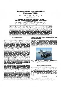
A unique suite of on-board sensors provide information related to the vehicle’s motion. The primary sensor is an inertial measurement unit that measures accelerations and angular rates in three dimensions. This sensor is reliable, but due to noise and unknown biases, it alone cannot provide sufficient navigational accuracy. Other sensors provide additional feedback. A Doppler velocity log provides velocities along four beam directions via acoustic Doppler measurements. An acoustic long baseline (LBL) system measures round-trip travel times between a transceiver on the vehicle and four transponder baseline stations at known locations. An attitude and pressure sensor complete the navigation suite. The attitude sensor provides orientation measurements, while the pressure sensor provides a sense of vehicle depth. We assume the platform-frame sensor locations are known exactly and that all measurements, except for the LBL, have negligible measurement latencies. Delay is inherent in the LBL system, and methods to address that delay to enhance navigation accuracy are a major contribution of this article. Figure 1 illustrates the general sensor configuration. Long baseline transceiver Attitude sensor Inertial measurement unit Pressure sensor
u p
Doppler velocity log r
q v
w
Figure 1: Vehicle sensor configuration.
1.2 NOTATION We use the following notation [5]. For vehicle position and attitude, define tangent plane position η1 = [x, y, z]⊤ and attitude η2 = [φ, θ, ψ]⊤ . Vehicle position is defined in local tangent plane coordinates, where x aligns with north, y aligns with east, and z is down. Euler attitude angles are roll (φ), pitch (θ), and yaw (ψ). In the vehicle or platform frame, define platform velocity ν1 = [u, v, w]⊤ , angular rates ν2 = [p, q, r]⊤ , and linear acceleration ap = [au , av , aw ]⊤ .
2.
MODEL DERIVATION
Given limited knowledge of system dynamics and environmental uncertainties, a kinematic model is often preferable to a complex dynamic model. More importantly, kinematics are exact, with no uncertain parameters. Dynamics are not. This kinematic model relates platform accelerations, velocities, and angular rates to changes in tangent plane position and attitude. It does not account for vehicle or fluid dynamics, or other environmental forces, thus allowing the navigation algorithms to be platform independent.
2
The inertial frame of reference i is at the Earth center and is non-accelerating, non-rotating, and has no gravitational field. The Earth-center/Earth-fixed (ECEF) frame e is coincident with and rotates about the inertial frame at a known constant rate, ωi/e . On the surface of the Earth lies tangent frame t, which is fixed within the ECEF frame. The inertial acceleration expressed in the tangent frame is h i ˙ t r t + r¨t , ai = Rti Ωti/t Ωti/t r t + 2Ωti/t r˙ t + Ω i/t
t ×] is the skew symmetric matrix form of rotation rate cross product of frame t where Ωti/t = [ωi/t with respect to frame i, represented in frame t. Vector r describes the vehicle position relative to the inertial origin. Solving for r¨t yields
˙ t rt r¨t = Rit ai − Ωti/t Ωti/t r t − 2Ωti/t r˙ t − Ω i/t
˙ t rt = Rit (f i + Gi ) − Ωti/t Ωti/t r t − 2Ωti/t r˙ t − Ω i/t ˙ t rt = f t + (Gt − Ωti/t Ωti/t r t ) − 2Ωti/t r˙ t − Ω i/t
(1)
= f t + gt − 2Ωti/e r˙ t ,
where vectors f and G represent the specific force and position dependent gravitational acceleration. Vector gt is the local gravity vector. Note that Ωi/t = Ωi/e + Ωe/t , and Ωe/t ≡ 0.
We use an Euler attitude representation to describe vehicle orientation, where an Euler 3-2-1 rotation sequence [6] defines the relationship between tangent and platform frames. It is important to understand that each Euler angle describes a rotation about an axis in separate frames. We exploit this relationship between intermediate frames in the formulation of attitude rates and in the measurement correction of attitude angles. The combined rotation sequence from tangent frame t to platform frame p is Rtp = R1 (φ)R2 (θ)R3 (ψ) cθcψ cθsψ −sθ = cψsθsφ − cφsψ cφcψ + sθsφsψ cθsφ , cφcψsθ + sφsψ −cψsφ + cφsθsψ cθcφ with inverse Rpt = (Rtp )−1 = (Rtp )⊤ . The velocity vectors in platform and tangent frames are related by v t = Rpt v p and v p = Rtp v t . (2) The time derivative of the second equation is v˙ p = Rtp v˙ t + R˙ tp v t = Rtp (f t + gt − 2Ωti/e v t ) + (−Ωpt/p Rtp )Rpt v p = ap − 2Ωpi/e v p − (Ωpi/p − Ωpi/e )v p
(3)
= ap − Rtp Ωti/e Rpt v p − Ωpi/p v p ,
where we have expressed v˙ t in the inertial frame using equation (1). Angular rate Ωpi/p is computed from the gyro measurement by removing biases. Platform acceleration ap is computed directly from the accelerometer specific force measurement by compensating for gravity and removing biases. Recall that each Euler angle defines a rotation about an axis in separate frames. To relate the ˙ θ, ˙ ψ) ˙ to angular rates in the platform frame, relate rotation axes (ˆı1 , ˆ2 , kˆ3 ) Euler attitude rates (φ, 3
in their respective intermediate frames to platform frame coordinates (ˆıp , ˆp , kˆp ). For example, [ˆıp , ˆp , kˆp ]⊤ = R2⊤ (θ)R1⊤ (ψ)[ˆı2 , ˆ2 , kˆ2 ]⊤ . Let p ˙ ı1 + θˆ ˙2 + ψ˙ kˆ3 ωt/p = φˆ
˙ ıp + θ(cφˆ ˙ p − sφkˆp ) − ψ(sθˆ ˙ ıp − cθsφˆ = φˆ p − cθcφkˆp ) ˙ ıp + (θcφ ˙ + ψcθsφ)ˆ ˙ ˙ ˙ kˆp = (φ˙ − ψsθ)ˆ p + (ψcθcφ − θsφ) be the vector expression of angular rates in platform frame p relative to the tangent frame t, represented in frame p. In matrix form and using notation from Section 1.2, the Euler and platform angular rates are related by ν2 = Ωη˙2 and η˙2 = Ω−1 ν2 ,
(4)
p p p ˙ θ, ˙ ψ] ˙ ⊤ , and where ν2 = ωt/p = ωi/p − ωi/e , η˙ 2 = [φ,
1 0 −sθ Ω = 0 cφ cθsφ . 0 −sφ cθcφ Note that the inverse relationship approaches a singularity as θ → ± π2 . It is assumed the vehicle will not operate near this singularity. If operation near ± π2 is desired, then an alternative attitude representation, such as quaternions, would remove this singularity. After equations (2)–(4) are summarized using the notation from Section 1.2, the continuous-time kinematic model is η˙1 = Rpt ν1 η˙2 = Ω−1 ν2 p
ν˙ 1 = a −
(5)
Rtp Ωti/e Rpt ν1
− Ωpi/p ν1 .
The next section utilizes this model, along with bias and measurement models, to propagate the system through time and formulate measurement predictions.
3.
NAVIGATION
Given system output y, we wish to reconstruct the entire internal state x. From linear systems theory, we know that if the discrete system xk+1 = Φxk + Γωk yk = Hxk is observable, then we can design the observer x ˆk+1 = Φˆ xk + L(yk − yˆk ) yˆk = H x ˆk
such that the eigenvalues of (Φ − LH) lie within the unit circle. This condition is necessary for asymptotic stability of the error state system, defined by δxk+1 = (Φ − LH)δxk δyk = Hδxk . 4
Asymptotic stability of the error state system causes δxk to converge exponentially to zero, thereby estimating xk . We use notation δxk , as opposed to x ˜k , to indicate the expected value of the error rather than the true error. For time-varying systems, Lk must stabilize (Φk − Lk Hk ) for all time [7, 8]. Here, we employ the Kalman filter to design Lk in an optimal manner, given noisy measurements y. The Kalman filter is optimal in the mean-squared sense [1, 2, 3]. In the following sections, we formulate system error state equations and apply the Kalman filter. Our formulation revolves around the system’s inertial measurement unit (IMU), and as such, we describe this sensor first in Section 3.1. Section 3.2 defines the augmented system equations. These equations model the true system, while Section 3.3 defines the mechanization equations that provide the navigation state vector x ˆ. The difference between the actual and mechanized systems is the error state system. A model for the error state system is described in Section 3.4. We use the error state system to design the Kalman filter. Section 3.5 applies the Kalman filter time propagation equations − δx− k+1 = Φk δxk − Pk+1
=
Φk Pk− Φ⊤ k
(6) + Qd ,
(7)
where equation (6) propagates the error state δx and equation (7) propagates the error state covariance Pk . Section 3.6 applies the Kalman filter measurement correction equations Kk = Pk− Hk⊤ (Hk Pk− Hk⊤ + Rk )−1
(8)
δyk = yk − h(ˆ xk )
(9)
δx+ k Pk+
=
δx− k
= (I −
+ Kk (δyk − Kk Hk )Pk− ,
Hk δx− k)
(10) (11)
to the aiding sensors. Equation (8) computes the optimal Kalman gain, equation (9) computes the measurement residual, equation (10) corrects the error state estimate, and equation (11) updates the error state covariance matrix. Circular (i.e., angular) measurements should correct the innovation − indicates the a priori state or covariance (δyk − Hδx− k ) to lie on interval [−π, π). Superscript at time k immediately prior to the innovation. Superscript + indicates the a posteriori state or covariance at time k immediately after the innovation. Kalman gain Kk is the optimal observer gain Lk at instant k. After a measurement correction, the filter should initialize the a priori state and covariance to the a posteriori state and covariance for the next filter iteration (i.e., x ˆ− ˆ+ k+1 = x k − and Pˆk+1 = Pˆk+ ). Recognizing the difference between the error state δx and navigation state x ˆ is important. The navigation mechanization computes x ˆ by integration of the IMU data between time instants tk and tk+1 , at which aiding measurements are available. At such time instants, x ˆ is used to predict the measurement. The filter uses the residual between the actual and predicted measurements to estimate δx+ . When δx+ is available, the navigation state x ˆ correction is x ˆ+ = x ˆ− + δx+ .
(12)
After each navigation state correction, error states δx− and δx+ are zero since the navigation state estimate now incorporates this information. Clearly, if we correct x ˆ immediately after each δx correction, δx− is always zero, and it is not necessary to propagate δx− as in equation (6).
5
3.1 INERTIAL MEASUREMENT UNIT The inertial measurement unit (IMU) is the primary high-rate sensor. It measures linear accelerations via accelerometers and angular rates via fiber-optic gyros. The IMU effective measurement point defines the origin of the platform frame. The IMU also provides an accurate time measurement since the last update. This delta time measurement is useful for precise integration, later described in Section 3.5. We expect this sensor to provide continuous updates without interruption. The accelerometer specific force and gyro measurement outputs, ya and yg , respectively, are modeled by ya = ap − Rtp gt + ba + na yg =
p ωi/p
+ bg + ng ,
(13a) (13b)
where (ba , na ) and (bg , ng ) are bias and noise vectors. Noise vectors na and nb are distributed according to N (0, σa2 I) and N (0, σb2 I), respectively, and are assumed to be white noise processes [1]. The acceleration and angular rate estimates are computed as ˆ p gt − ˆba a ˆ p = ya + R (14a) t
p ω ˆ i/p
= yg − ˆbg .
(14b)
Bias vectors ba and bg are modeled as random constants plus random walks, where ˆb˙ a = 0 ˆb˙ g = 0.
b˙ a = ωa b˙ g = ωg
(15a) (15b)
2 I) and N (0, σ 2 I), respecThe driving noise vectors ωa and ωg are distributed according to N (0, σba bg tively.
3.2 AUGMENTED SYSTEM EQUATIONS Augmenting our continuous-time model, in equation (5), with the models for the unknown parameters in equations (15a) and (15b), yields the system state vector � �⊤ b⊤ c x = η1⊤ η2⊤ ν1⊤ b⊤ . a g The additional parameter c represents our estimate for the speed of sound in seawater. We model c as a random constant plus random walk with driving noise ωc ∼ N (0, σc2 ), where σc = 0.1 m/s. This estimate is necessary to calculate round-trip distances from travel times for the long baseline system, described in Section 3.6.3. The process noise input vector is � �⊤ n⊤ ωa⊤ ωg⊤ ωc u = n⊤ , a g
where all quantities are mutually uncorrelated, Gaussian, white noise vectors. The augmented true system equations are therefore η˙ 1 = Rpt ν1 t η˙ 2 = Ω−1 (yg − bg − ng − Rtp ωi/e )
ν˙ 1 = (ya + Rtp gt − ba − na ) − Rtp Ωti/e Rpt ν1 − (yg − bg − ng ) × ν1 b˙ a = ωa b˙ g = ωg
c˙ = ωc , 6
(16)
where we have substituted for ap and ν2 with equations (14a) and (14b), respectively, in preparation for the development of the error state equations in Section 3.4. 3.3 MECHANIZATION EQUATIONS The mechanization equations represent the expected value of the true system. Our estimate of the true system, equation (16), is ˆ t νˆ1 ηˆ˙ 1 = R p ˙ηˆ2 = Ω ˆ −1 (yg − ˆbg − R ˆ pωt ) t i/e
ˆ p gt − ˆba ) − R ˆ p Ωt R ˆ p ˆ1 − (yg − ˆbg ) × νˆ1 νˆ˙ 1 = (ya + R t t i/e t ν ˆb˙ a = 0 ˆb˙ g = 0 cˆ˙ = 0,
(17)
where we assume the gravitation vector gt and rotation rate Ωti/e are deterministic. 3.4 ERROR STATE EQUATIONS The error state equations represent the expected value of the error between the true system and its estimate, δx˙ = x˙ − x ˆ˙ . To compute the transformation error between two rotation matrices, we ˆ t = (I − [δρ×])Rt , where (I − [δρ×]) represents a smalldefine a small-angle transformation as R p p angle transformation from the true tangent frame to the computed tangent frame [9]. The quantity δρ represents the small-angle error between true and computed frames. The error state vector is then � �⊤ δb⊤ δc δx = δη1⊤ δρ⊤ δν1⊤ δb⊤ , (18) a g where δρ replaces δη2 . The following relations are useful in the subsequent analysis; ˆ pt = (I − [δρ×])Rpt R ˆpt Rpt = (I + [δρ×])R ˆp R t Rtp
= =
Rtp (I ˆ p (I R t
(19a) (19b)
+ [δρ×])
(19c)
− [δρ×]).
(19d)
Using the small-angle relationships, we compute the error state equations for each state. The tangent position error is δη˙1 = η˙ 1 − ηˆ˙1 ˆ pt δν1 + [δρ×]R ˆpt δν1 + [δρ×]R ˆpt νˆ1 (20) =R ˆ pt δν1 − [R ˆ pt νˆ1 ×]δρ, ≈R where we have manipulated the terms such that the error state coefficients can be represented in matrix form. To determine the error state model for δρ˙ [10], differentiate the rotation matrix error δRpt = [δρ×]Rpt , t ˙t δR˙ pt = [δρ×]R ˙ p + [δρ×]Rp t t p = [δρ×]R ˙ p + [δρ×](Rp Ωt/p ),
7
and solve for [δρ×], ˙ ˆ˙ t )Rp − [δρ×]Rt Ωp Rp [δρ×] ˙ = (R˙ pt − R p p t/p t t
ˆ pt Ω ˆ p )Rp − [δρ×]Ωt = (Rpt Ωpt/p − R t t/p t/p
t ˆp R ˆp ˆ pt Ω = Ωtt/p − R t/p t (I − [δρ×]) − [δρ×]Ωt/p
ˆt + Ω ˆ t [δρ×] − [δρ×]Ω ˆt . ≈ Ωtt/p − Ω t/p t/p t/p Equivalently, this expression written in vector form is t t t δρ˙ = ωt/p −ω ˆ t/p +ω ˆ t/p × δρ
p p t t ˆt ω ˆt ˆ p − ω = Rpt ωi/p −R ˆ i/t ) × δρ p ˆ i/p − δωi/t + (Rp ω i/p
t ˆ t δω p + [δρ×]R ˆ t δω p − δω t − ω =R ˆ i/t × δρ p p i/t i/p i/p
(21)
t ˆ t (−δbg − ng ) − δω t − ω ≈R ˆ i/t × δρ, p i/t
t = {−ω [sin φ, ¯ 0, cos φ] ¯ ⊤ ∂ φ/∂η ¯ ¯ where δωi/t 1 }δη1 and φ is the vehicle latitude. The platform velocity i/e error is δν˙ 1 = ν˙ 1 − νˆ˙ 1 o n ˆ p [gt ×] + ω t (R ˆ t νˆ1 )⊤ − (ω t · R ˆ t νˆ1 )I δρ ≈R p p t i/e i/e n o (22) ˆ p Ωt R ˆ pt δν1 − δba − na − [(yg − ˆbg )×] + R t i/e
ˆ p δgt + R ˆ p [R ˆ t νˆ1 ×]δω t . − [ˆ ν1 ×]δbg − [ˆ ν1 ×]ng + R p t t i/e
Remaining error expressions for δba , δbg , and δc are trivial and, as such, their derivation is not shown. The resulting continuous-time error state system is δx˙ = F δx + Gu, where
F =
(23)
ˆ pt νˆ1 ×] R ˆ pt 0 −[R 0 0 t ˆt F21 −Ωi/e 0 0 −R p F31 F32 F33 −I −[ˆ ν1 ×] 0 0 0 0 0 0 0 0 0 0 0 0 0 0 0
0 0 0 0 0 0
t /∂η1 F21 = ∂ωi/t n o ˆ p ∂gt /∂η1 + [R ˆ pt νˆ1 ×]∂ω t /∂η1 F31 = R t i/e n o ˆ p [gt ×] + ω t (R ˆ pt νˆ1 )⊤ − (ω t · R ˆ pt νˆ1 )I F32 = R t i/e i/e
ˆ p Ωt R ˆt F33 = −[(yg − ˆbg )×] − R t i/e p
and
G=
0 0 ˆ pt 0 −R −I −[ˆ ν1 ×] 0 0 0 0 0 0 8
0 0 0 I 0 0
0 0 0 0 I 0
0 0 0 0 0 I
.
Due to the relatively small operating area, we assume F21 and F31 are approximately zero. Note that the error state vector contains δρ, while the navigation state contains η2 . The measurement correction routines in Section 3.6 will account for the use of δρ. 3.5 TIME PROPAGATION The time propagation routine propagates the navigation state, error state, and error state covariance through time. For each measurement update from the IMU, the time propagation routine computes the continuous-time system, the discrete-time system, and then propagates the system state and covariance. The continuous-time system is F and G with process noise distribution matrix Q, where matrices F and G are computed according to equation (23) and Q = Ehuu⊤ i. We assume 2 I, σ 2 I, σ 2 ). To compute the equivalent discrete-time system, we compute Q = diag(σa2 I, σb2 I, σba c bg the matrix exponential � � �� −F GQG⊤ △t Υ = exp 0 F⊤ using algorithms from reference [11]. Quantity △t is the integration period from the IMU. The result is � � −D Φ−1 Qd Υ= , 0 Φ⊤ where matrices Φ and Qd represent the discrete-time system [12]. Matrix Φ(k + 1, k) propagates − − − −⊤ the error state δx− k and covariance Pk , where Pk = Ehδxk δxk i, from time k to k + 1 according to equations (6) and (7), respectively. Matrix Qd represents the discrete-time process noise distribution matrix at time k, and D is a nonzero dummy matrix. Given Υ, matrices Φ and Qd are trivially solved from its sub-matrices, Φ(k + 1, k) = Υ[n + 1 : 2n, n + 1 : 2n]⊤ Qd (k) = Φ(k + 1, k)Υ[1 : n, n + 1 : 2n],
(24) (25)
where Υ[r1 : r2 , c1 : c2 ] represents rows r1 through r2 and columns c1 through c2 of the 2n × 2n matrix Υ. We propagate the navigation state estimate x ˆ− using a predictor-corrector integration algorithm [13], − xpk+1 = x− k + f (xk , yk )△t p xck+1 = x− k + f (xk+1 , yk )△t 1 p c x− k+1 = 2 (xk+1 + xk+1 ),
(26)
where yk = [ya (k), yg (k)]⊤ , then correct the resulting attitude angles to lie on interval [−π, π). Function f (x, y) is the continuous-time mechanization described in equation (17). 3.6 MEASUREMENT CORRECTIONS In this section, we use the terms sensor and measurement to refer to all sensors other than the IMU. These aiding sensors are discussed in Sections 3.6.1 through 3.6.4. Each sensor runs independent of the next, with its own update rate and performance characteristics. Thus, measurement corrections are asynchronous. As a measurement arrives, it is evaluated and then incorporated into the error state estimate. If a measurement does not arrive, no calculations are necessary. The algorithm does 9
not wait for or expect measurements to arrive in an ordered fashion; the error state and navigation state will propagate according to equations (6) and (26), respectively, via the IMU data, with or without measurement corrections. Measurements are evaluated with several sanity checks. One such check verifies that the mea− ⊤ 2 surement lies within three standard deviations of its estimate, (δyk − Hk δx− k ) < 9(Hk Pk Hk + Rk ), − ⊤ where δyk is the measurement residual and matrix (Hk Pk Hk + Rk ) represents the measurement covariance. Additional logic is necessary to help ensure that this algorithm does not disregard valid measurements, especially upon initialization. Valid measurements correct the error state estimate according to equation (10). The following sections describe the low-rate aiding sensors and their respective measurement correction. Measurement corrections require a measurement residual δy, sensor output matrix H, and measurement noise matrix R to evaluate equations (8) and (10). Note that the error state vector contains δρ, while the navigation state vector contains ηˆ2 . We cannot simply correct the attitude states of x ˆ, ˆ p via (19d), as described in equation (12). Instead, we use ηˆ2− to correct transformation matrix R t where + ˆ p (ˆ ˆ p η − )(I − [δρ×]), R (27) t η2 ) = Rt (ˆ 2 and compute ηˆ2+ from the resulting transformation matrix, � � ˆ p [2, 3], R ˆp [3, 3] φˆ+ = arctan2 R t t
(28a)
ˆ p [1, 3] R t � �2 ˆ p [1, 3] 1− R t � � ˆ p [1, 2], R ˆp [1, 1] , ψˆ+ = arctan2 R t t θˆ+ = − arctan r
(28b)
(28c)
+ ˆ p [i, j] represents the (i, j) element of matrix R ˆ p (ˆ where R t t η2 ) [12]. Function arctan2(y, x) is the ˆp four-quadrant arc tangent function. To ensure numerical stability, it is necessary to normalize R t prior to evaluating equations (28a)–(28c).
3.6.1 Attitude Update The attitude sensor combines four tilt and three magnetometer measurements to produce roll, pitch, and yaw information. We assume the vehicle dynamics are slow, and as such, the coupling between the inclinometers and platform acceleration is negligible. We also assume the magnetometer is calibrated to compensate for hard iron characteristics of the operating region. Momentary magnetic spikes can easily be ignored. The sensor model is ye = η2 + ne , where sensor noise ne is distributed according to N (0, σe2 I). We can predict the measurement as yˆe = ηˆ2 , and compute the measurement residual as δye = ye − yˆe 10
(29)
when a measurement arrives. To formulate the sensor output matrix H and measurement noise matrix R, a theoretical expression for the measurement residual must be determined in terms of the error state. In this case, an expression for δη2 in terms of δρ must be found. This formulation is similar to the relationship between the Euler attitude rates and platform angular rates. Quantity δη2 describes attitude error relative to the intermediate rotation axes (ˆı1 , ˆ2 , kˆ3 ), while δρ describes attitude error in tangent frame (ˆıt , ˆt , kˆt ). By definition, δρ = δφˆı1 + δθˆ 2 + δψ kˆ3 = δφ(cθcψˆıt + cθsψˆ t − sθ kˆt ) − δθ(sψˆıt − cψˆ t ) + δψ kˆt
= (δφcθcψ − δθsψ)ˆıt + (δφcθsψ + δθcψ)ˆ t + (δψ − δφsθ)kˆt = Σδη2 , where
cθcψ −sψ 0 Σ = cθsψ cψ 0 . −sθ 0 1
The theoretical measurement error expression is therefore η2 } δye = {η2 + ne } − {ˆ = Σ−1 δρ + ne = Hδx + ne , where the sensor output matrix is H=
�
0 Σ−1 0 0 0 0
�
.
Note that Σ−1 approaches a singularity as θ → ± π2 . The measurement noise matrix is D E R = E δyδy ⊤ D E ⊤ = E ne ne
(30)
(31)
= σe2 I,
which is positive definite for all time. Quantities Hδx and R represent the mean and covariance, respectively, of the distribution for δy. When an attitude measurement arrives, the Kalman filter evaluates equations (29)–(31) and then uses the results in (8)–(12), and (28a)–(28c) to correct the state estimate. Note that the Kalman filter assumes δρ is small; therefore, the attitude sensor should initialize ηˆ2 with the latest measurement when the filter initializes. In Section 4.1, we show that yaw is observable from the long baseline system when the vehicle has a nonzero velocity, thus the magnetic compass can be disabled if necessary. 3.6.2 Doppler Velocity Log Update The Doppler velocity log (DVL) measures velocity via the Doppler effect by first emitting encoded acoustic pulses from each of its four transducer heads. These pulses reflect off surfaces, such as the seafloor, and return back to each transducer. The instrument measures the change in frequency between the pulses emitted and those received, which relates to velocities along each 11
beam direction relative to the reflecting object. In certain situations, one or more beams may not return valid information. When fewer than three beams return valid information, we cannot compute geometric transformation [14] to relate beam velocities to instrument frame velocities. It is possible to alleviate this restriction. Here, we treat each beam velocity as a separate innovation. This approach does not require bottom lock and incorporates more information into the filter than an instrument frame correction (i.e., four beam corrections vs. three orthogonal corrections). is
Let b = {b1 , b2 , b3 , b4 } be unit vectors along each beam direction. The ith Doppler measurement yv = (ν1 + ν2 × ℓi ) · bi + nv ,
which represents the instrument frame velocity along beam direction bi . Vector ℓi is the transducer head offset from the origin of the platform frame, and nv is sensor noise with normal distribution N (0, σv2 ). The measurement estimate is therefore ν1 + νˆ2 × ℓi ) · bi , yˆv = (ˆ where ℓi and bi are known exactly, with residual δyv = yv − yˆv
(32)
ν1 + νˆ2 × ℓi ) · bi } = {(ν1 + ν2 × ℓi ) · bi + nv } − {(ˆ ⊤ ⊤ = b⊤ i δν1 + bi [ℓi ×]δbg + bi [ℓi ×]δng + nv .
The sensor output matrix is H=
h
i ⊤ [ℓ ×] 0 , 0 0 b⊤ 0 b i i i
and the measurement noise matrix is �n on o⊤ � ⊤ ⊤ R=E bi [ℓi ×]ng + nv bi [ℓi ×]ng + nv =
2 ⊤ b⊤ i [ℓi ×]σg I[ℓi ×] bi
+
(33)
(34)
σv2 ,
which is positive definite for all time. Note the significance of the sensor placement in relation to the gyro bias and variance. Offset ℓi provides observability to the gyro bias in equation (33), while ℓ2i magnifies the effect of the gyro variance in equation (34). We ignore any correlation between the process noise ng and measurement noise vectors. When a DVL beam measurement arrives, the Kalman filter evaluates equations (32)–(34) and then uses the results in (8)–(12), and (28a)–(28c) to correct the state estimate. Each beam provides a separate measurement correction. 3.6.3 Long Baseline Update The acoustic long baseline (LBL) system precisely measures the time of flight of sound waves propagating through water. At time t0 , the vehicle transceiver generates a common interrogate ping. Each listening transponder hears this ping, each at a different time, then waits a specified turn-around time and responds. For example, transponder 1 responds 250 ms after hearing the ping, transponder 2 responds at 500 ms, followed by transponder 3 at 750 ms, and finally transponder 4 at 1000 ms after hearing the ping. No two transponders respond at the same time, allowing the the turn-around time to identify the transponder. The vehicle receives the response from the ith transponder at time ti . Figure 2 illustrates the interrogation cycle. 12
Ti
Pi
P (t0 ) P (ti )
Figure 2: Long baseline interrogation cycle. Dotted lines indicate the acoustic measurement. The solid line indicates an arbitrary vehicle trajectory.
The total round-trip time for the ith transponder measurement is the travel time to the transponder plus the return travel time plus the turn-around time plus noise, or
1 1
yt =
Pi − P (t0 ) +
Pi − P (ti ) + Ti + nt , c(t0 ) c(ti )
where c(t) is the speed of sound in seawater and position vectors Pi and P (t) represent the position of transponder i and the vehicle transceiver at time t, respectively. The vehicle transceiver position in tangent frame is P = η1 + Rpt ℓ, where ℓ is the sensor offset from the platform origin. Constant Ti is the transponder turn-around time. Sensor noise nt is distributed according to N (0, σt2 ). The measurement estimate is therefore
1 1
ˆ ˆ yˆt = − P (t ) + − P (t )
Pi
Pi 0 i + Ti , cˆ(t0 ) cˆ(ti )
where the transponder position Pi and turn-around time Ti are known. The algorithm stores the current state estimate at time t0 , then recalls it to compute measurement residual δyt = yt − yˆt
(35)
1 at time ti . We address the nonlinear 2-norm expression d(t) = c(t) kPi − P (t)k by representing it using a first-order Taylor series approximation about state estimate x ˆ, ∂d 1 ∂2d d = dˆ + ⊤ (x − x ˆ) + ˆ)2 + . . . (x − x ∂x xˆ 2! (∂x2 )⊤ xˆ ∂d ≈ dˆ + ⊤ δx. ∂x xˆ The dependence on state estimates at two separate times complicates the formulation of the measurement residual. It is necessary to relate the error state backwards in time to the common interrogate ping via state transition matrix Φ(t0 , ti ). The measurement residual is then n o n o ˆ 0 ) + d(t ˆ i ) + Ti yt = d(t0 ) + d(ti ) + Ti + nt − d(t h i h i ˆ 0 ) + d(ti ) − d(t ˆ i ) + nt = d(t0 ) − d(t ∂d(t0 ) ∂d(ti ) ≈ δx(t0 ) + δx(ti ) + nt ∂x⊤ xˆ(t0 ) ∂x⊤ xˆ(ti ) h i = D(t0 )Φ(t0 , ti ) + D(ti ) δx(ti ) + nt ,
13
where the sensor output matrix is H = D(t0 )Φ(t0 , ti ) + D(ti ).
(36)
State transition matrix Φ(t0 , ti ) propagates the error state backwards in time from time ti to t0 . At each time step, from time t0 to ti , the time propagation routine accumulates transition matrix Φ(ti , t0 ) according to Φ(t + △t, t0 ) = Φ(t + △t, t)Φ(t, t0 ), where Φ(t + △t, t) is given by equation (24). When a measurement arrives, the measurement correction routine computes the inverse relationship, where Φ(t0 , ti ) = Φ−1 (ti , t0 ), and applies the measurement correction. The nonzero partial derivative terms of matrix D(t) are ∂d(t) 1 (Pi − Pˆ (t))⊤ = − cˆ(t) kPi − Pˆ (t)k ∂η1⊤ xˆ ∂d(t) 1 (Pi − Pˆ (t))⊤ ˆ t = [R (t)ℓ×] ∂ρ⊤ xˆ cˆ(t) kPi − Pˆ (t)k p
1 ∂d(t)
ˆ P = − − P (t)
. i ∂c cˆ2 (t) x ˆ
The measurement noise matrix is
D E R = E nt n⊤ = σt2 , t
(37)
which is a positive scalar for all time. When the vehicle transceiver emits a common interrogate ping, the correction routine stores the current state estimate, while the time propagation routine begins accumulating the state transition matrix. During this time, the filter does not correct the navigation state according to equation (12) until the last transponder measurement arrives. This practice is necessary such that we can relate δx(ti ) to δx(t0 ) via Φ(t0 , ti ). All intermediate corrections, including those from other aiding sensors, propagate in δx− . When a measurement arrives, the Kalman filter evaluates equations (35)–(37) and then uses the results in equations (8)–(11) to correct the error state. When the last transponder measurement arrives, the filter corrects the navigation state according to equation (12) and equations (28a)–(28c). Timeout logic is necessary to handle the situation where the last measurement does not arrive. After all transponders reply or timeout, the cycle repeats. To ensure stability during the initialization process, we initialize diagonal elements of P0|0 relating to δη1 and δc artificially small. 3.6.4 Pressure Update Over the vehicle’s operating depths, the Saunders and Fofonoff (1976) relationship [15] between pressure and depth is nearly linear, thus we model the pressure sensor as yz = s(η1 + Rpt ℓ) + bz + nz , where s and bz scale and offset the pressure measurement, respectively, and s = [0, 0, sz ]. Vector ℓ is the sensor position in platform frame. Sensor noise nz is distributed according to N (0, σz2 ). The measurement prediction is then ˆ pt ℓ) + bz , yˆz = s(ˆ η1 + R where we assume constants sz and bz are known. Therefore, the residual can be calculated as δyz = yz − yˆz
(38)
ˆ pt ℓ) + bz } = {s(η1 + Rpt ℓ) + bz + nz } − {s(ˆ η1 + R ˆ pt ℓ×]δρ + nz . = sδη1 − s[R 14
The sensor output matrix is then H=
h
ˆ pt ℓ×] 0 0 0 0 s −s[R
i
(39)
with a measurement noise matrix of D E R = E nz n⊤ = σz2 , z
(40)
which is a positive scalar for all time. When a pressure measurement arrives, the Kalman filter evaluates equations (38)–(40) and then uses the results in equations (8)–(12), and equations (28a)– (28c) to correct the state estimate.
4.
ANALYSIS
To analyze our filter implementation, we examine the navigation state error, covariance, and measurement residuals. Here, we consider several scenarios in simulation and study the navigation state error and covariance. In Section 5, we evaluate the measurement residuals for experimental data. The navigation state error x ˜, which is only available when the true navigation state is available, substantiates the filter’s performance. The objective is to drive the navigation state error to zero. The covariance matrix provides a performance estimate of δx, where the square root of the diagonal describes the error state standard deviation. We expect the navigation state error to remain within three standard deviations of zero. The measurement residuals describe the performance of the filter’s measurement predictions. These residuals should be white noise when the system and measurement models approximate the true system. The vehicle simulation is comprehensive. It models a three-dimensional environment, sensor performance, vehicle dynamics, and executes the actual vehicle software to approximate real-world performance. The sensor models are similar to those presented above, where in addition to measurement noise, we incorporate sporadic sensor dropouts and those due to poor geometry and loss of line of sight. Acoustic sensor models are simple. We do not attempt to model acoustic sound propagation or multi-path effects, and we assume that acoustic transmissions are instantaneous with respect to the simulation step size. The vehicle model accounts for vehicle dynamics, hydrodynamics, currents, and thruster forces based on experimental data. For analysis purposes, we assume this model represents the truth model. It is helpful to understand the observability of the system for analysis. Observability analysis allows one to determine if it is possible to estimate the error state δx from the output y. Given system matrix F and a measurement output matrix H, we can compute observability matrix O to determine the states made observable via the measurement correction associated with H. Unobservable states may remain constant or diverge, depending on the model and time propagation routine. The rate of divergence deserves future discussion. To check observability, construct the observability matrix H HF O= , .. . HF n−1
where matrix H is a measurement output matrix or combination of multiple measurement output matrices H = [H1⊤ , H2⊤ , . . . ]⊤ . The rank of O indicates the number of error states observable; if 15
O is full rank, we can estimate the entire error state from output y [7, 8]. The dimension of our system is 16, thus a rank of 16 is necessary to estimate δx. The rank of O is complementary to the dimension of the unobservable subspace. Clearly, O depends on x for nonlinear systems. We assume nominal conditions (ˆ x = [0, 0, 0, 0, 0, 1500]⊤ ) unless stated. The scenarios of interest are where different combinations of acoustic sensors drop out. These sensors, which include the LBL and DVL, are highly susceptible to interference, so it is important to examine the effect when their respective measurements are unavailable. For each scenario, the vehicle submerges to 5 m in depth, and then executes a lawnmower search pattern. The leg length is 40 m, with a row spacing of 5 m. After nine consecutive rows, the vehicle returns to the beginning of the first row and repeats the mission. The vehicle speed is 0.5 m/s. The acoustic baseline outlines a 50 × 50 m2 box around the operating area. Figure 3 illustrates the mission trajectory. The true initial conditions are normally distributed about zero with realistic variances, except for the vehicle yaw angle and the speed of sound. Yaw is uniformly distributed about a circle, and speed of sound is normally distributed about 1450 m/s with variance (15 m/s)2 . All initial estimates are zero or the first available measurement, except for the speed of sound, which is 1500 m/s. For the nominal case, the system has full observability, thus we expect to estimate δx and therefore x when all sensors are functioning. 50
40
North (m)
30
20
10
0
-10 -10
0
10
20
30
40
50
East (m)
Figure 3: North–East plot of one simulated mission from the incremental LBL dropout scenario, where the solid line represents the navigation estimate and the dashed line represents the true trajectory. The four circles represent the LBL transponders. For comparison, the small dots represent three and four-range trilateralization solutions.
All results represent the average of 100 Monte Carlo simulations. The error plots illustrate the true navigation state error x ˜ and the corresponding standard deviation estimate of δx (divided by 10). All δx divergence rates are for one standard deviation. Our observability analysis assumes ωi/e ≈ 0 to eliminate the attitude observability gained from the rotation of the Earth.
16
4.1 INCREMENTAL LBL DROPOUTS, LIMITED COMPASS AIDING First, consider the ship-hull inspection scenario. Operators place one LBL transponder at each corner of a ship and deploy an inspection vehicle. The vehicle executes several passes around and underneath the hull, searching for objects of interest. In this scenario, the keel frequently obstructs line of sight between the vehicle and one or more transponders, and, due to magnetic anomalies, vehicles typically operate without a magnetic compass. To illustrate the system performance in this scenario, we sequentially drop out LBL transponders. Transponder one fails at 600 seconds, followed by transponders two, three, and four at 1200, 1800, and 2400 seconds, respectively. Yaw aiding is only available during the first 30 seconds of the mission, which allows the algorithm to estimate η2 such that δρ becomes small before disabling the compass. The DVL, pressure, and inclinometers continue to aid the system. Figures 4, 5, and 6 illustrate the performance of the east position, azimuth, and speed of sound error states, respectively. On interval t ∈ [30, 600) seconds, where four transponders are responding and the compass is disabled, the nominal system has rank(O) = 15. The unobservable subspace Σu spans linear combinations of {δη1 (x, y), δρ(ψ)}. This result is intuitive. Clearly, we cannot observe azimuth when the vehicle is stationary. Observability analysis indicates that velocity in the horizontal direction promotes O to full rank; vertical velocity does not. Vehicle rotation, where ν2 (r) 6= 0, also promotes O to full rank.
The loss of one transponder does not affect the observability of the nominal system. The unobservable subspace remains unchanged. Velocity in the horizontal direction promotes O to full rank. Rotating, however, does not promote O to full rank. The unobservable subspace transforms where linear combinations of {δη1 (x, y), δρ(ψ), δc} are not observable. Eliminating δc from the error state vector allows this maneuver to achieve full observability. Losing two transponders increases the dimension of Σu to 2, where Σu spans linear combinations of {δη1 (x, y), δρ(ψ), δc}. Velocity in the horizontal direction no longer achieves full observability. The algorithm cannot differentiate between certain linear combinations of δη1 (x, y) and δc. To im0.25 7.2 mm/s
Average true error η˜1 (y) (m)
0.2
5.5 mm/s
0.15 0.1 0.05 0 -0.05 -0.1 -0.15
η˜1 (y)
δη1 (y) 3σ
-0.2 -0.25
0
500
1000
1500 2000 Time (s)
2500
3000
Figure 4: East position error η˜1 (y) for incremental LBL transponder dropouts and limited compass aiding. LBL transponders drop out at multiples of 600 seconds. The oscillations in standard deviation correlate to the vehicle trajectory and its relationship to each transponder.
17
0.5 Average true error ρ˜(ψ) (deg)
0.4
δρ(ψ) 3σ
0.3
ρ˜(ψ)
0.2 0.1 0 -0.1 -0.2
0.87 × 10⁻³ deg/s
-0.3 -0.4 -0.5
1.5 × 10⁻³ deg/s 0
500
1000
1500 2000 Time (s)
2500
3000
Figure 5: Azimuth error ρ˜(ψ) for incremental LBL transponder dropouts and limited compass aiding. LBL transponders drop out at multiples of 600 seconds. The true azimuth error is computed using equation (19a).
Average true error c˜ (m/s)
0 δc 3σ
-5
Slow divergence
1.5 mm/s2
c˜
-10 -15 -20 -25
0
500
1000
1500 2000 Time (s)
2500
3000
Figure 6: Sound speed error c˜ for incremental LBL transponder dropouts and limited compass aiding. LBL transponders drop out at multiples of 600 seconds.
prove results, one could invest in aiding sensors for δc or assume the speed of sound is deterministic. Elimination of δc from the error state vector makes O full rank for nonzero horizontal velocities. For small operating regions, assuming a constant sound speed may produce acceptable results. Figure 6 shows that the covariance of δc converges prior to the loss of the second transponder. Since the driving noise is small, the Kalman gain K is small and the estimate remains steady over interval t ∈ [1200, 1800) seconds. The loss of the third transponder results in divergence. Figures 4 and 5 indicate the divergence rates for east position error and azimuth error, respectively. On interval t ∈ [1800, 2400) seconds, where only one transponder operates, rank(O) = 13 for zero velocity and Σu spans linear combinations of {δη1 (x, y), δρ(ψ), δc}. For nonzero horizontal velocities, rank(O) = 14 and Σu spans linear 18
combinations of {δη1 (x, y), δc}. Losing all transponders reduces observability to 11 states and Σu spans linear combinations of {δη1 (x, y), δρ(ψ)}, {δbg (ψ)}, and {δc}. Note that as kPi − Pˆ (t)k → 0 in equation (36), δc becomes weakly observable. Thus, for small area searches such as the scenario presented here, the algorithm may be unable to estimate δc accurately as a result of the LBL sensor performance characteristics. We assume σt = 1.0 ms and σc = 0.1 m/s. Figure 6 shows that we cannot estimate the true speed of sound within 5 m/s for the given scenario. 4.2 INCREMENTAL DVL BEAM DROPOUTS, NO LBL AIDING Consider the scenario when the LBL sensor is unavailable and the DVL begins to malfunction. Beam one fails at 200 seconds, followed by beams two, three, and four at 400, 600, and 800 seconds, respectively. The attitude and pressure sensors continue to aid the system. Figures 7 and 8 depict the performance of velocity error ν˜1 (u) and accelerometer bias error ˜ba (u). Initially, the north and east error states, as well as the speed of sound, are not observable, and rank(O) = 13. The unobservable subspace spans linear combinations of {δη1 (x, y)} and {δc}. This result is expected since no sensors aid position or speed of sound. When beam one fails, there is no additional loss in observability. Subspace Σu transforms, but the general relationships remain the same. Figure 7 shows only a slight decrease in performance. 0.03 Average true error ν˜1 (u) (m/s)
δν1 (u) 3σ 0.02 ν˜1 (u)
0.01 0 -0.01
3.1 mm/s2
-0.02 -0.03
2.3 mm/s2 5.5 mm/s2 0
100 200 300 400 500 600 700 800 900 1000 Time (s)
Figure 7: Velocity error ν˜1 (u) for incremental DVL beam dropouts and no LBL aiding. DVL beams drop out at multiples of 200 seconds.
19
Average true error ˜ba (u) (mm/s2 )
5 ˜ba (u)
4 3 2 1 0 -1 -2
2.4 × 10⁻³ mm/s3
-3 δb (u) 3σ a -4 -5
0
100 200 300 400 500 600 700 800 900 1000 Time (s)
Figure 8: Accelerometer bias error ˜ba (u) for incremental DVL beam dropouts and no LBL aiding. DVL beams drop out at multiples of 200 seconds.
The performance resulting for a loss of a second beam depends on the particular beam lost. If the remaining beams lie within perpendicular planes, the unobservable subspace remains the same dimension and the performance loss is subtle. If the remaining beams lie within the same plane, the effect is detrimental. Our simulation reveals this condition, where the dimension of Σu increases to 5 and the rank of O drops to 11. Linear combinations of {δη1 (x, y), δν1 , δba } and {δc} are not observable. From Figure 7, we see that sometimes the system excites observable modes and the error state and covariance briefly converge. To understand this behavior, we perform a separate observability analysis for different conditions. For nonzero velocity, such as when the vehicle is tracking the segment between two waypoints, Σu has dimension 5. For nonzero angular rates, such as when the vehicle achieves a waypoint and maneuvers towards the next waypoint, Σu has dimension 4. Linear combinations of {δη1 (x, y), δν1 , δba } and {δc} are not observable for both cases. Finally, when the vehicle has a nonzero roll or pitch angle, Σu has dimension 3. For this condition, the unobservable subspace is similar to a single beam failure. The oscillations in Figure 7 correspond to the trajectory of the vehicle. At each waypoint, the vehicle maneuvers (with nonzero angular rates, and a slight roll angle) towards the next waypoint and the solution converges. When tracking the segment between two waypoints, the solution diverges. Losing a third beam is similar to the previous case, where the dimension of Σu is 5. The performance loss is subtle over interval t ∈ [600, 800). The divergence rates are comparable to a two-beam failure. A total loss of the DVL causes divergence rates to increase. The divergence rate corresponding to velocity error δν1 (u) is 5.5 mm/s2 and to accelerometer bias error δba (u) is 2.4 × 10⁻³ mm/s3 . The rank of O drops to 9 states, and the system can no longer maintain an acceptable level of performance. Note that this scenario illustrates the worst case. Intermittent beam dropouts result in only a slight decrease in performance due to an effective lower update rate.
20
5.
EXPERIMENTAL RESULTS
The following experimental results are from a demonstration at the Autonomous Underwater Vehicle Festival (AUVFest) in 2007. The mission plan was to submerge to 3 m in depth for 2 minutes, then execute two sets of three-dimensional waypoints at 1 knot. The first series of waypoints consisted of vertically stacked legs between two waypoints. During this phase, the navigational goal was to observe the unknown parameters (yaw and biases) before proceeding to the second series of waypoints underneath a barge. The second series of waypoints consisted of a lawnmower search pattern in an continuous loop, similar to the scenario presented in Section 4. Due to severe magnetic interference from the barge, we chose to operate the vehicle without aiding the yaw angle with the magnetic compass. The acoustic baseline outlines a 36 × 9 m2 box around the second series of waypoints. Since the true state is not available, we present analysis of select error state covariances and measurement residuals. Note that the sensor data presented here is identical to that presented in reference [4]; however, here we reprocessed the raw data through the algorithms presented in this report. Position accuracy is a critical metric for inspection-class vehicles. This information allows operators to localize objects of interest, reacquire contacts, and navigation through complex environments. Figure 9 illustrates the estimated standard deviation of the north, east, and down error states during the AUVFest demonstration. These results are consistent with the simulation results in Figure 4. The convergence is dependent on the acoustic baseline geometry, vehicle trajectory, and several important factors. These factors include accuracy of the baseline calibration, estimate of the speed of sound, and the estimate of the vehicle attitude. 0.45 δη1 standard deviation (m)
0.4 0.35
δη1 (y) 1σ
0.3 0.25 0.2 0.15 0.1
0
δη1 (z) 1σ
δη1 (x) 1σ
0.05 0
500
1000 1500 Time (s)
2000
2500
Figure 9: North, east, and down position error δη1 standard deviation. The standard deviation estimate converges to 13 cm, 17 cm, and 0.7 cm for north, east, and down position errors, respectively. These results are subject to the baseline configuration and do not necessarily mean η˜1 is this accurate.
We determine the acoustic baseline geometry prior to deployment via acoustic calibration. Using a spare transponder, the calibration algorithm measures round-trip travel times to each transponder and among all transponders. The algorithm assumes the relative organization of transponders to formulate a geometric solution, which provides estimates for the transponder locations and the speed of sound. For our demonstration, it estimated a sound speed of 1491 m/s. The transponder 21
locations are in a local coordinate system, where transponder 1 identifies the origin and the vector from transponder 1 to transponder 3 defines the y-axis. We transform these coordinates into tangent plane coordinates for navigation. The current hardware implementation requires us to perform this procedure prior to operating the vehicle. It is not possible to estimate the baseline online with our current hardware. Clearly, a poor baseline calibration will degrade performance. Analyzing the LBL round-trip measurement residuals provides insight into the baseline calibration. Figure 10 represents the measurement residuals for transponder 1. Several features are apparent. First, the residuals do not resemble white noise. Second, approximately 7 percent of the data lies beyond three standard deviations of its expected value. We attribute these erroneous measurements to acoustic noise and multi-path effects. Simple filtering techniques tend to produce inconsistent results due to the slow update rate and position uncertainty. Our current algorithm assumes all measurements are valid. Another notable feature evident in the data is a profound oscillation. This oscillation is evident in all transponder residuals and is consistent with a poor baseline calibration in simulation. Simulation results confirm that misalignment of one transponder will hinder performance of the entire system. The oscillation correlates to the vehicle trajectory. Figure 9 also shows an oscillatory pattern in the north and east error state standard deviations.
LBL transponder 1 residual (ms)
14 12 10 8 6 4 2 0 -2 -4
0
500
1000 1500 Time (s)
2000
2500
Figure 10: Long baseline transponder 1 residual. This residual exhibits an oscillatory pattern that is consistent with baseline misalignment and the vehicle trajectory. All transponder residuals exhibit √ similar patterns. The horizontal lines indicate one, two, and three standard deviations about zero, where σ = HP − H ⊤ + R.
Inaccuracies in the speed of sound estimate can also cause oscillations in the round-trip measurement residuals. Figure 11 illustrates the estimate of the speed of sound. The calibration routine estimated 1491 m/s. The navigation algorithm, however, converged near 1420 m/s, which is unrealistic, given environmental conditions. Possible explanations include unknown biases, scale factors, and inaccuracies in the sensor clock frequency. The azimuth error is of particular interest since yaw is an essential control signal and δρ(ψ) is only observable via the long baseline system. Poor estimation of error state δρ(ψ), and δρ, generally, will result in inadequate navigation and control performance. Figure 12 illustrates the azimuth and corresponding gyro bias error standard deviations. The azimuth error δρ(ψ) standard deviation converges to 0.5 deg. This result does not necessarily mean ρ˜(ψ) is this accurate, however, it is consistent with the simulation results in Figure 5. Note that the performance specifications for our 22
Speed of sound estimate cˆ (m/s)
1500 1490 1480 1470
cˆ ± 3σ
1460 1450
cˆ
1440 1430 1420 1410 1400
0
500
1000 1500 Time (s)
2000
2500
Figure 11: Sound speed estimate cˆ. Thin lines indicate three standard deviations beyond the estimate. The estimate converges to approximately 1420 m/s, which is suspicious, given the environmental conditions. 1
fiber-optic gyro include a bias stability of