Autonomous Waypoint Selection for Navigation and Path Planning: A Navigation Framework for Multiple Planning Algorithms Sanjeev Sharma and Matthew E. Taylor Abstract— This paper introduces a novel waypoints selection framework for autonomous navigation in unknown and continuous environments, which may use a number of existing path planners. The Autonomous Waypoint Selection Framework (AWSF) is domain- and space-independent framework, which selects waypoints within an agent’s field-of-view. Each waypoint is treated as a temporary goal location, allowing the agent to eventually reach the goal state. Using AWSF, both local and global path planning algorithms can be used for online local waypoint planning. The key benefits of AWSF are: (i) allowing the agent to navigate in unknown and unseen spaces, using waypoints, with any path planning algorithm; (ii) significantly reducing planning time of existing planners by reducing the workspace; and (iii) learning in 2D spaces but automatically generalizing to planning in 3D-spaces. We empirically evaluate our framework with 5 path planning algorithms: an A? planner, an unconstrained cubic spline interpolation in both 2D- and 3Dspaces, the 2D- and 3D-ECAN planners, and a MILP-based dynamically feasible trajectory planner.
I. I NTRODUCTION Attempting to deploy robots and unmanned vehicles in uncertain and unknown environments has become an increasingly popular. Despite recent successes such as the NASA Mars Rovers [1] and the DARPA Grand Challenges, navigation in completely unknown and unseen environments remains a difficult problem. Such robots should intelligently determine a feasible direction while avoiding obstacles, eventually reaching the goal location. Recent work in both vision and AI-based methods [2]–[4] have focused on determining a navigation direction based on a set of identifiable signatures or landmarks in known, partially known, or unknown environments. However, in extremely difficult conditions (for example a UAV or an off-road UGV navigating in unknown environment), no such symbols or signatures are available, and determining a feasible direction can be equivalently described as finding the waypoint or nearby temporary goal location. Waypoints tell the robot (or, equivalently, the agent) where to navigate so that it may make progress towards the goal location. From a planning perspective, selecting nearby waypoints allows a path planning algorithm to focus on a very small part of the environment, significantly reducing the computational burden of path or trajectory (motion) planning in large environments. Previous research in path planning and navigation has developed highly efficient path and motion planners. We broadly classify them as local or global planners. Local Sanjeev Sharma is a graduate student in the Dept. of Computing Science, University of Alberta, Canada:
[email protected] Matthew E. Taylor is an assistant professor in the Dept. of Computer Science, Lafayette College, USA:
[email protected]
planners (e.g., [5]–[9]) require little or no prior knowledge of the environment and (re-) planning is performed online. Global planners (e.g., [10]–[13]), although highly efficient, require complete knowledge of the environment before planning takes place, which may preclude their use in unknown environments. Recent years have also seen a growing interest in using Mixed-Integer Linear Programming (MILP) formulations for planning dynamically feasible trajectories (motion). However, MILP based planning is often restricted to known environments, and planning in partially known environments assumes determinism [31]. Since MILP is NPHard in the number of binary variables, re-planning in large environments can be computationally expensive. We aim to circumvent these problems by autonomously generating the waypoints in the robot’s field-of-view (FOV). The primary motivation for generating such waypoints is that global planners can treat them as goal locations and quickly plan a path to the next waypoint, allowing global planners to be used in unknown and unseen environment. Allowing both local and global planners to focus on small regions of the entire space significantly improves planning speed, possibly at the expense of plan performance. The Autonomous Waypoint Selection Framework (AWSF) is a novel domain-independent framework that selects waypoints in unknown and unseen spaces. AWSF uses information in the agent’s FOV and geometric features of the environment (discussed in Section III). Additionally, because AWSF is domain-independent, the robot may be trained in one domain and then tested in another, including training in a 2D space and being tested in a 3D space. To allow such generalization, we create a local planningspace (LPS) that can be used to plan in both 2D and 3D, motivated by the agent-space [15] formulation. This technique is particularly valuable when it is more difficult to collect 3D-space data, compared to 2D-space data, which is often the case. As motivation, consider how a human navigates in a previously unseen environment. A human may perceive obstacles in a space similarly, whether he is walking, driving a car, or flying an airplane. LPS enables the agent to make higher level decisions (selecting the waypoints) for the path planning algorithm, regardless of the dimensionality of the planning space. Path planning algorithms generate a path to reach to the next waypoint (see Fig. 1). Henceforth we use agent to describe a single entity whose decisions are governed by two internal RL-agents. At each time-step (Fig. 1), the agent observes its state, as observed in its FOV. The state includes the position and the density of obstacles in the form of local potential fields. This local information
agent navigating in
2D or 3D environment
Reward Function Local & Global Information Extraction
RL-Agents LPS 𝛷1 , 𝛷2
Information Extraction Waypoints Path Planning
Fig. 1: Domain and space independent autonomous waypoints selection framework (AWSF) with 2 internal RL-agents
is then further processed and combined with global information (Section III) to form the space, LPS, allowing the internal RL-agents to perceive the navigation problem in the same way, irrespective of the particular domain or space. LPS is then used to determine the number and location of (future) waypoints in the agent’s FOV (Fig. 1). We empirically show the key benefits of AWSF, including: (i) global planners can be used in unknown spaces, (ii) planning time may be reduced by as much as three orders of magnitude, and (iii) training in a 2D-space may be used by an agent in a 3D-space (and vice versa). Experiments (Section V) investigate the performance with five planners: A? (a global grid-planner), unconstrained cubic spline interpolation (a fast local planner), 2D- and 3D-ECAN (local planners [14]), and a global MILP-based motion planner. II. R ELATED WORK This section presents a selection of work most related to AWSF. Similar to the agent-space idea, Busquets et al. [3] modeled the observation-space of an agent by constructing a network of landmarks, but the approach is restricted to environments where a full model may be learned. Frommberger et al. [16]–[18] proposed the GRLPR and le-RLPR frameworks, which use an idea similar to agent-space, for producing navigation strategies in semantically similar situations. However, reaching the goal location depended on recognizable landmarks (i.e., colored walls), and the method may require retraining in new domains, often making it inapplicable in unseen spaces. In contrast, AWSF is domain independent and is capable of inter-space planning (e.g., learning to plan in 2D and then planning in 3D). As explained in the following section, we construct potential fields based on the surroundings of the agent. The use of potential fields and range readings for mapping the surroundings is a well-studied area. Our approach to potential fields is most closely related to utilizing range readings for classifying safe regions for the robot [1], as potential fields in LPS help to determine safe-regions for waypoints. Sharma et al. [19] presented a global waypoint selection strategy, but required a pre-specified path based on userdefined waypoints. Randomized motion planners like RRTs [20] explore the environment by randomly sampling it for constructing trees. Recent work [21] has successfully applied RRTs for online planning, but the approach required a nearby location to be specified on the road for expanding the trees in a particular direction. In contrast, AWSF intelligently provides a temporary goal location and may therefore provide a much more efficient navigation in general 2D- and 3D-spaces.
Recent work in local path set generation in 2Dspaces [22]–[24] has focused on incrementally generating a feasible motion trajectory by planning locally at each time step, towards the goal location. AWSF considers every possibly reachable portion of the region in robot’s FOV and then selects most appropriate regions (waypoints) in the FOV for incremental planning in 2D- and 3D-spaces. AWSF may improve the computational performance of pathset methods by considering only those trajectories that end near the waypoint. However, empirical results contrasting the proposed framework from the path-set generation methods is beyond the scope of this paper. III. LPS IN AWSF FOR D EFINING WAYPOINT ( S ) For the purpose of this paper, we assume that the agent: (i) cannot see beyond its FOV, (ii) knows its location (zat ) at each time-step t (e.g., most outdoor vehicles can use GPS to find their coordinates), and (iii) knows coordinates (ztgl ) of the target goal location (TGL). This section describes the construction of LPS for waypoint selection in 2D- and 3D-spaces. As described earlier, the agent has two internal RL agents. These internal RL agents (Fig. 1) use different state representations, using both local (agent’s observation) and global (i.e., goal location) information. The two RL agents allow multiple path planning algorithms (hereafter, “planners”) to be integrated into AWSF. One internal agent, A1 , generates the waypoints in the environment, independent of the planner used. The other agent, A2 , captures behavior of planners by deciding the number of waypoints to be selected (ntw ) at each time-step (t). Together they check collision when the planner is inherently incapable of avoiding the collisions. The next sections describe how LPS is constructed from the local and global information.1 A. Extracting Local Information: Agent’s Observation The agent’s observations are described by two local potential fields, a point-map (PM) and an edge-map (EM), which are used to construct the LPS. Since we do not restrict AWSF to a specific planner, we consider both point-obstacles and finite-obstacles. When using a grid-based planner (e.g., A? ), each point obstacle is represented as occupying one complete grid cell. At each time-step t, the PM and EM represent the local region in the agent’s FOV. To form these maps, the agent’s FOV is discretized. Using a polar coordinate system, we denote the agent’s view by hRFOV , θFOV i in 2D-spaces and by hRFOV , θFOV , φFOV i in 3D-spaces. The FOV is thus defined by hr, θi and hr, θ, φi in 2D- and 3D-spaces respectively, where r ∈ (0, RFOV ], θ ∈ [−θFOV , +θFOV ] and φ ∈ [−φFOV , +φFOV ]. The parameters dr, dθ, and dφ represent the discretization of respective components. The total number of grid points, N , in the FOV is ((2θFOV + 1)RFOV )/(dr.dθ) in 2D-spaces and ((2θFOV + 1)(2φFOV + 1)RFOV )/(dr.dθ.dφ) in 3D-spaces. Obstacles lying in the agent’s FOV are then used to compute PM (for point-obstacles) and EM (for finite-obstacles), 1 An implementation of AWSF in MATLAB and Python will be soon available for download at http://www.searching-eye.com/awsf/.
(a)
(b)
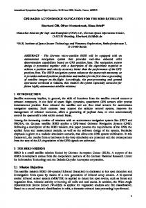
Fig. 2: (a) shows EM and (b) shows PM, where red regions represents higher values relative to blue regions. direction of navigation
agent
grid-point
gj r
Obstacle Unknown area and out of agent’s View
d gj r tgl
i 1; i {1,..., nwt }
Fig. 3: The left figure shows two geometric parameters for A1 . The right figure shows a situation where the parameter ζji = 1 for all grid-points which lie above the obstacle (red-triangle) and to left of the red-line.
30 20
for each of the grid-points in the agent’s FOV. Higher values correspond to closer proximity to an obstacle. For EM, when finite-obstacles are discovered in the FOV, then grid 35 the 40 45 50 points lying on their boundaries/edges are marked as edgeobstacles to compute EM. For m point-obstacles and n edge25 30 35 40 45 50 obstacles in the agent’s FOV, the value of each of the N grid points in PM and EM is computed as: Pm Pn ||lq −lj ||22 ||lq −lj ||22 ) e j=1 exp(− j=1 exp(− 1.5σ ) σ2 p Vq ← ; Vq ← max(V p ) max(V e ) (1) where q = {1, ..., N }; Vqe , Vqp ∈ R+ ∪ {0} are values of the q th grid point in EM and PM respectively; and lq and lj are locations of the q th grid point and the j th (point or N ∪ {0} edge-obstacle) obstacle, respectively. V e , V p ∈ R+ p are vectors of grid point values. If m = 0 then Vq = 0; if n = 0 then Vqe = 0, ∀q = {1, ..., N }. Next, values for grid points corresponding to edge-obstacles are set to 1 in PM. Fig. 2 shows PM and EM for a 2D-space. B. Environment Representations for Constructing LPS The PM and EM are then combined with local and global geometric parameters for local planning-space (LPS) construction, described in this section. Two different state representations, Φ1 and Φ2 , are constructed simultaneously, forming LPS (Φ1 , Φ2 ). A1 then uses Φ1 and A2 uses Φ2 to make decisions. The next two subsections describe how Φ1 and Φ2 are constructed by combining the local and global information and using function approximation (our implementation uses Fourier basis functions [25]). LPS is thus constructed using information readily available during navigation. Additionally, no space-specific (2D or 3D) information is used: the parameters are normalized and computed identically for different space dimensionalities. C. Φ1 Construction in LPS for A1 : Selecting Waypoints To construct Φ1 , three geometric parameters are computed that combine local and global information (see Fig. 1) with local potential fields. Two of the parameters measure the progress towards the goal location if the j th grid point is j to be selected as the waypoint. The first, θgr ∈ [−π, π), is the angle between the vectors connecting zat to ztgl and zat to the j th grid point (lj ). The second is the normalized
distance of the j th grid point from TGL, ρjgr = (djgr /ω), where djgr = ||ztgl − lj ||2 and ω = 10||za0 − ztgl ||2 (za0 is the agent’s location at t = 0). Fig. 3 (left) depicts these parameters. The third parameter (ζji ) is a Boolean parameter that identifies potentially unsafe regions for the waypoints. This third parameter determines whether a line-segment between the ith -waypoint and the j th grid point intersects finite-obstacle. Let zat and lj are the locations of the agent and the j th grid point. Now, suppose that A1 has to select 2 waypoints — ζj0 and ζj1 must be computed. ζj0 (for the j th grid point) is 1 if the line-segment joining zat and lj intersects finite-size obstacle and zero otherwise. After selecting the first waypoint (one of the grid points in the FOV), A1 must determine the second waypoint. Now, ζj1 = 1 (for the j th grid point) if the line-segment joining the 1st waypoint and lj intersects finite-size obstacle, and is zero otherwise. If there is an obstacle between the agent and the j th grid point (Fig. 3, right), ζji = 1, ∀i = 1, . . . , (ntw − 1). Regions that are completely unknown and hidden from view are thus marked as potentially unsafe. ζ is most helpful when using a planner that cannot inherently avoid collisions, like unconstrained spline interpolation, but are very fast and useful in high-speed navigation. j A parameter vector xij = [Vjs , θgr /π, ρjgr , Vje , ζji ]T , is deth fined for the j grid-point for selecting the (i+1)th waypoint; i = 0, . . . , (ntw − 1). We use Fourier basis functions [25] for combining the parameters to produce the representation Φ1 for A1 .2 We use fourth-order uncoupled Fourier basis for the first 3 parameters of xij and first-order uncoupled basis for ζji , leading to 13 uncoupled Fourier basis functions for the j th grid-point. We use first-order coupling [25] to j with ρjgr and Vje with ζji . Also, we append Vje couple θgr and a constant term 1 to the Fourier basis. Thus, each of the grid-points is parameterized by a basis function vector Φ1 (xij ) ∈ R17 ; j = {1, ..., N }. This vector represents the state-action basis function, where actions correspond to selecting a particular grid-point as the waypoint. Reinforcement learning methods [26] are then used to learn a near-optimal policy (see Section IV). D. Φ2 Construction for A2 : Number of Waypoints A2 must select ntw at time t using the Φ2 part of LPS as its state. Like Φ1 , Φ2 also models both the local and global information. A2 ’s action space consists of ntw actions. We limit ntw to 3, i.e. A2 has 3 possible actions. Φ2 is constructed by embedding a parameter vector yt = t [(λt /π), ρt , vm , ψ t , Ωt , δ t ]T in Fourier functions. Here λt ∈ [−π, π) is the angle between a vector from zat to ztgl and a vector defining the agent’s navigation direction at time t; ρt = (||zat − ztgl ||2 )/(2||za0 − ztgl ||2 ) is the normalized PN t distance of the agent to the goal; vm = ( j=1 Vjp /N ); ψ t is number of point-obstacles in the FOV divided by 10; 2 We expect that other kernel-based function approximators, as well as different orders for the chosen Fourier basis functions, will also perform well. We chose orders according to complexity of parameters and leave a detailed exploration of this implementation detail to future work.
Ωt ∈ [0, 1] is the entropy3 of PM divided by maximum possible entropy (i.e., 8); and δ t measures fraction of space in the FOV covered by finite-obstacles at time t (including obstructed unseen space). The first two parameters in yt effectively measure the agent’s deviation and distance from the goal location. The last 4 parameters measure how cluttered the local region is, and Ωt measures how randomly the obstacles are distributed in the FOV. A more cluttered space may require more waypoints for efficient path planning. After computing yt , we use Fourier basis to represent the state-space (Φ2 ) for A2 . We use fourth-order uncoupled basis functions for first 5 parameters of yt and second-order uncoupled basis for δ t . This yields 22 uncoupled bases. We t t use second-order coupling to couple vm with Ωt , vm with t t t ψ , Ω with ψ and first-order coupling to couple ω t with ρt . This leads to 13 coupled Fourier basis functions. We append a constant 1 to the basis function vector. Thus the state-basis function vector for A2 at time t is a vector ∈ R36 . The state-action basis function (Φ2 (yt )) is then formed by copying state-basis for each of the actions (see [26], [28]. IV. R EINFORCEMENT L EARNING : A1 AND A2 We use the Markov decision process framework for solving the underlying reinforcement learning (RL) problem, learning (near-) optimal policies for A1 and A2 . In RL [26], a value function Qπ (s, a) for a policy π predicts the longterm reward if an agent takes action a ∈ A in state s ∈ S and thereafter follows policy π : S → A. The agent’s probability of taking action a in s is given by π(s, a). An agent’s task is to learn a policy π that maximizes total expected reward from any s ∈ S, which may be discounted by some γ ∈ [0, 1). By taking action a in s, agent makes a transition to state s0 , receives an a reward from R(s). We approximate the valuefunction using a linear function approximation architecture, where Q(s, a) = φ(s, a)T w is approximated with a stateaction basis vector φ(s, a) ∈ Rk , where Φ1 (xij ) is used for A1 and Φ2 (yt ) is used for A2 , and w ∈ Rk is learned using samples. The reward function is designed to help A1 generate waypoints and for A2 to decide the appropriate number of waypoints. Using this reward function, A1 learns to operate independently of the planner, guiding the agent quickly to the goal location (TGL) and A2 learns to decide ntw for the planner in use. At each time t, A1 defines ntw waypoints. When ntw = 1, the waypoint is one of the grid points in the FOV. When ntw = 2, the first waypoint lies in a region with radius [0, R2FOV ] and the second lies in a region with radius ( R2FOV , RFOV ]. Similarly, with 3 waypoints, the FOV is divided into three regions and the one waypoint is selected in each region. For selecting the j th grid-point as ith -waypoint, A1 receives a reward: ri = −103 ζji−1 −2ωpi −min(10, 103 ωfi )+max(αg (500, −5)). 3 Entropy is computed by converting PM to a gray-scale image — each grid point (a pixel in the image) assumes a discrete value in {0, ..., 255}; entropy of discrete parameter (e.g., here grid point or pixel) is maximum if its probability distribution function is uniform.
Here αg = 1 if the waypoint is defined at TGL and −1 otherwise; ωpi and ωfi compute the waypoint’s value in PM and EM, using equations 1, where (σ ← 0.5657σ) for PM and (σ ← 0.3017σ 2 ) for EM. A2 learns a policy to select ntw and receives a reward based on the path generated by the planner. The resulting path, planned by continuous planners, is discretized in a step of 0.1-units, giving a total of qdiscrete points (which is the path-length). A? gives a discrete path with grid-cells; for computing the reward, its length is measured as the number of grid-cells traveled to reach the waypoints. The reward for A2 at time-step t is: rt = −ntw − qαpath −
q X (ωpj + ωfj ). j=1
Here ωpj and ωfj compute the j th discretized point’s (on the path) value as described above for the waypoints; αpath = 1 for A? and 0.05 for all other planners. Selecting the number of waypoints balances a performance with computation. A2 gets penalized with −ntw for selecting multiple waypoints as it requires computing ζji for each waypoint. However, in heavily cluttered environments, the penalty (ωpj and ωfj ) associated with close proximity to obstacles will outweigh the penalty of −ntw and A2 will select more waypoints.4 V. E XPERIMENTS This section empirically evaluates claims made throughout the paper. Five planning algorithms have been selected to demonstrate the capabilities of the AWSF framework. We denote algorithms used in AWSF with a wp subscript (for waypoint)—A? in AWSF is A?wp . We discuss planning time comparisons and compare path-lengths for A?wp and MILPwp with A? (Section V-A) and MILP (Section VD), respectively. With ECANwp (Section V-C), we discuss computational and planning advantages, and with UCSIwp (Section V-B) we show that AWSF can avoid collisions even with a planner that cannot inherently avoid collisions. We use Q-learning [27] for learning A1 ’s policy and LSPI [28] for learning A2 ’s policy. In both cases, the discount factor is defined to be γ = 0.9. These learned policies are domain independent—we first learn A1 ’s policy in multiple 2D-domains with randomly generated pointobstacles ranging from 10 to 450 and with finite-obstacles occupying 10% to 50% of the total space. Once A1 has learned its policy, A2 trains in either 2D or 3D-spaces (depending on the algorithm). After training A1 and A2 , the complete framework can be deployed in any environment. We use the following default parameter values: hRFOV , dr, φFOV , dφ, σ 2 i = h5, 0.2, 40◦ , 2◦ , 0.5i. Values of θFOV , and dθ are 60◦ and 1◦ (2D), or 40◦ and 2◦ (3D). All MILP based experiments were performed on a Windows-7 notebook computer with a 2.66GHz Core-i5 processor in MATLAB using AMPL and CPLEX. All other experiments were done on a Windows-7 desktop computer with a 3.10GHz Core-i3 processor using 4 In our experiments we show path planned with AWSF with 3-different color to show A2 ’s action — situations where A2 selects more waypoints
50 45
Point−obst Waypoint A*wp:1−wp
40
A*wp:2−wp
35
A*wp:3−wp A*
30 25 20 15 10 5 0 0
5
10
15
20
25
30
35
40
45
50
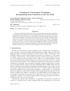
Fig. 4: This figure compares paths planned with A?wp and A? . Line colors show when A?wp uses from one (1-wp) to three (3-wp) waypoints.
the number of waypoints (Wp) selected by A2 , while using A?wp , by using multiple color paths. The incremental path planned with A?wp is close to the global-optimal path, and A?wp path is also not too close to the boundary of obstacles — AWSF plans successfully with A? . Fig. 5 compares the planning time and path-length (measured as euclidean distance) of A?wp and A? . When planning in same size environment (x-axis of Fig. 5) and with the same granularity (as measured by the ratio of number of grid-cells in the same area), A?wp is three orders of magnitude faster than A? . However, in our experimental domains, paths planned with A?wp are longer than those planned with A? . Experiments tested two different cases where 25% and 58% of the area was covered by obstacles, averaged over 15-tasks for each case.
0.9 3
0.8 0.7 0.6
2
10
0.5 0.4 1
10
Time:(A*/A*wp)−Avg Occp Area:25%
0.3
Ratio of Average Path−Length: A*/A*wp
Ratio of Average Planning Time: A*/A*wp
10
Time:−Avg Occp Area:58% *
Path−Length:(A /A*wp)−Avg
Occp Area:25% 0.2
Path−Length:−Avg Occp Area:58%
0
10
0
0.1 0.1 0.2 0.3 0.4 0.5 0.6 0.7 0.8 0.9 1 Ratio of Granularity (Ratio of number of grid−cells in a given area): A*/A*wp
Fig. 5: This figure shows that in the same size environment A?wp can be three orders of magnitude faster and planning time is same when A?wp plans in ≈ 28.2 times larger environment than A? . Paths planned with A?wp (with zero-prior knowledge) are slightly longer than A? paths.
MATLAB with CVX [30] (for ECAN planners). We show the ratio of the average planning-time and the average path-length to show the efficiency of planning with AWSF. Furthermore, we also report the planning time of AWSF separately to show extremely fast re-planning of the waypoints. A. Planning using A? with and without AWSF For the standard A? implementation, a grid-based planner, the 50 × 50 unit2 environment was discretized uniformly in the x and y directions. This discretization varies from 0.093units to 0.5-units, creating environments of different size (granularity). Point-obstacles were represented as entirely covering the nearest grid-cell in the map. A?wp uses parameters dr, dθ and produces 3,025 grid points in the agent’s FOV at every time-step. These points are then converted to a 121 × 25 map for planning with A?wp , providing 121 heading-directions that are 1◦ -apart, while A? has only 8 heading-directions. Thus, the length of the A?wp path is comparable to that of the global-optimal path planned with A? . Fig. 4 shows sample paths produced by A?wp with no prior knowledge and the A? with complete knowledge of the environment, TGLs are at (30, 50) and (48, 33), and 501 point-obstacles have been added randomly. Fig. 4 also shows
B. Inter-Space Planning and Using an Unconstrained Planner This section shows that AWSF can be combined with UCSI, which is technically not a planning algorithm. However, we use UCSI to show (i) the robustness of AWSF and (ii) that AWSF can leverage UCSI to efficiently plan paths in uncluttered (sparse) spaces. We use both 2D- and 3D-UCSI but, since they both plan in the same way, A2 learned a policy for only 2D-UCSI and then uses that policy in both 2D- and 3D-spaces. We do not use any advanced computations (e.g., [29]) to suppress the overshooting of cubic interpolation, relying instead on selected waypoints for collision avoidance. Our emphasis is to show a worst case scenario for AWSF by using a planner that does not have any inherent collision avoidance. When AWSF correctly places waypoints to avoid collisions, UCSI can be used as a very fast (re-) planner, such as when a UAV must navigate at high-speeds. Fig. 6 shows planning with 2D-UCSIwp in a challenging environment that is made more difficult by adding 301 randomly generated point-obstacles. Fig. 7 shows efficient planning with 3DUCSIwp using policies (for both A1 and A2 ) learned by training in 2D-spaces. Together, these results show that AWSF can plan in challenging environments, with waypoints, by using a planner that cannot inherently avoid collisions. Additionally, we show that waypoints planning in a 3D-space is possible by utilizing a policy learned in 2D-spaces. C. AWSF with 2D and 3D-ECAN: Local Planners Experiments in this section demonstrate AWSF’s performance using local online planning algorithms, as well as the inter-space planning ability of A1 .5 Without loss of generality, we assume a point-mass agent for ECAN [14] planners. ECAN is particularly attractive because its planning time does not depended on the size of the planning environment, but we can show that AWSF planning is comparatively faster as it allows (i) ECAN to focus on reaching nearby waypoints and (ii) waypoints to help avoid collisions. All the ECAN 5 A ’s policy was learned in 2D- and 3D-spaces for 2D- and 3D-ECAN 2 respectively, as A2 is planner-specific, while A1 learned only in 2D-spaces.
50 45 40
45
ECANwp:2−wp 40
35
35
30
30
25
25
20
20
15
15
TGL: (30,50) (46,50)
5
5 0
0 0
5
10
15
20
25
30
35
40
45
50
Fig. 6: AWSF enables UCSI to plan in an unknown and unseen cluttered 2D-space from 3 different starting positions, with 2 different goal locations.
20 Start:(0,0,0) tgl(50,50,10) Spline:1−wp Waypoint
z−axis
16 14 12 10 8 6 4 2 0 0
ECANwp:3−wp
10
10
18
Point Obst Waypoint ECANwp:1−wp
50
Start (1,1);(24,2) (2.05,12.35) Point Obst Waypoint Spline: 1−wp
y−axis 40
x−axis 10
20
30
20 40
50
0
Fig. 7: This figure shows 3D-UCSIwp planning with zero prior knowledge.
parameters, except the field-of-view and discretization parameters, were same as in previous work [14]. ECAN planners are useful for path planning in open environments, such as in Fig. 4, but perform poorly in closed spaces like the one in Fig. 6. Our results show that AWSF efficiently extended 2D-ECAN to such environments (Fig. 8), both with and without point-obstacles. Without waypoints, ECAN did not reach the TGL as it failed to successfully execute U -turns required at many locations. This is because when the goal location is far away, the principal axis of the ellipsoid, formed at each step [14] (which decides the navigation direction), points towards the TGL rather than the open regions. This results in local oscillations. With waypoints, ECAN receives a temporary goal location which guides the ellipsoid tunnel to the TGL. Hence the navigation with 2D-ECANwp is very efficient. Fig. 9a shows sample results from planning in unseen and cluttered space with 3D-ECANwp . 0–104 random pointobstacles were generated with an increment of 100-obstacles in each environment (resulting in 101 cluttered environments) in a (50 × 50 × 20) unit3 region containing 14 3Dobstacles. Planning with 3D-ECAN alone failed to reach the goal location in these environments, while 3D-ECANwp reached goal location in all each of the 101-environments (100% success). With AWSF and ECAN, grid points lying on finite obstacles can be removed from the constraints as
0
5
10
15
20
25
30
35
40
45
50
Fig. 8: AWSF can plan in cluttered, unknown spaces with 2D-ECAN (ECANwp ). Start and goal states are identical to that used in Fig. 6.
the generated waypoints implicitly take obstacle avoidance into consideration. Therefore, when only finite-obstacles are present in the environment, ellipsoid formation step ([14]) requires only 3 convex constraints, while 3D-ECAN can require up to 1200 constraints. The average time of ellipsoid formation step in 3D-ECANwp is 0.0985 seconds, while 3DECAN alone requires an average of 0.1387 seconds. Also, ECANwp often does not need to determine a navigation direction inside each planning ellipsoid. This is because the waypoint often lies on the boundary of ellipsoid, thereby trivially providing the navigation direction. This may save 0.3849 seconds, at each time-step, in obstacle dense regions. Thus 3D-ECANwp may be as much as 530% faster in cluttered spaces than 3D-ECAN alone. D. Scalable MILP Planning in Unknown Environments Experiments in this section address two issues of current MILP-based planning algorithms: (i) AWSF enables MILP planning to scale to large environments with many obstacles, and (ii) AWSF allows MILP planners to operate even with zero-prior knowledge of the environment. Our experiments use standard MATLAB code6 for MILP implementation (others [10], [11] have provided overviews of the StandardMILP formulation). Our results focus on 2D-spaces, but should extend to 3D-spaces as well. For planning with MILP, we set ntw = 1. We test MILPwp in 50 × 50 unit2 environment, where the agent’s maximum possible speed is vmax = 0.5 unit (resulting in reasonable size environments) s and a maximum angular velocity of ωmax = 15 rad s . To avoid confusion between the AWSF time-step and MILP time-step, we denote time for latter as tm . The MILP uses time-steps dtm = 0.2 seconds and a time-step in AWSF refers to the waypoint selection. At each time-step t, AWSF selects a waypoint. In MILP, “time” refers to the navigation time, and dtm is the resolution for formulating the MILP. At each time-step t, AWSF solves a MILP for planning a dynamically feasible path to reach the waypoint. A maximum number of time-steps (dtm ) allowed for reaching the 6 Trajectory optimization code was provided by the MIT Aerospace Controls Lab in MATLAB with an AMPL and CPLEX interface: http: //acl.mit.edu/milp/.
Start(0,0,0) Point−Obst tgl:(50,50,10) ECANwp:1−wp ECANwp:2−wp ECANwp:3−wp
0
X−axis 10 20 20 10 30
Z−axis 0
40
Y−axis 0
10
20
30
(a)
50
y
waypoint at time-step t was set to Tt = [(dwp /(vmax dtm ))] + [40dwp ]; dwp is the distance between the agent and the waypoint; and [.] is the greatest integer function. After solving the MILP at time t, we record the number (Tt ) of time-steps out of Tt time-steps required for reaching the waypoint, which we term active steps. When MILP plans with full knowledge of the environP ment, we set the time-step limit to t Tt . This is because the path planned with MILP will never be longer than the path planned with MILPwp — MILPwp gives an upper-bound on the required time-steps for MILP. Once solved, we record the number of active steps in MILP. Active steps actually measure the navigation time (and approximately the pathlength). Fig. 10 shows sample trajectories, comparing the zero-knowledge based planner MILPwp with full knowledge based planner MILP. Experiments show that MILPwp is able to avoid collision with gradually discovered obstacles in the FOV at several locations. Fig. 11 compares ratios of average planning time and of average path-length, averaged over 200tasks (20 tasks for each obstacle). Our results show that: (i) MILPwp can plan dynamically feasible paths, (ii) MILPwp complexity does not significantly increase with the environment size or number of obstacles due to local waypoint planning, (iii) the path produced with MILPwp is close to the global-optimal path; and (iv) MILPwp can be successfully applied to completely unknown spaces. We note that recent work, Tunnel-MILP [11], also decreases the number of integer variables to some extent, but is a global planner. Schouwenaars et al. [31] presented a loiter circle to navigate with limited visibility but requires a deterministic and static environment in the visible region. In dynamic environments, MILPwp can quickly re-plan the waypoints and does not rely on this assumption.
45
45
40
40
35
35
30
30
25
25
20
20
15
15
10
10
5 0
40
50
50
50
Y−axis
5
0
5
10
15
20
25 x
30
35
40
45
0 50 0
X−axis 5
(b)
10
15
20
25
30
35
40
45
50
(c)
Fig. 9: (a) planning in unseen-cluttered 3D-space with 3D-ECANwp , showing that A1 uses the policy learned in 2D-spaces to plan waypoints in a 3D-space (ii); (b) projection of Fig 7; and (c) projection of Fig 9a on the x-y plane 50
Start tgl MILPwp
45 40
MILP
35 30 25 20 15
E. AWSF: Fast Planning and Re-planning 10
The time AWSF requires to locate waypoints is the planning time of AWSF (or, inversely, the re-planning frequency). For 2D-spaces, we experimented in domains with 10-60% obstacle occupied area. This resulted in a total of 7198iterations of AWSF framework (summing AWSF-iterations required for reaching the goal location in each domain). The computational time of potential fields is more problematic in dense regions of the environment. In our experimental domains, we measured a lower bound on the re-planning frequency was 15.65Hz and the upper bound was 56.24Hz. The average re-planning frequency was 29.23Hz, with mean time for computing potential fields as 0.0274 seconds. Computing Φ1 and allowing A1 to make a decision took an average time of 0.0029 seconds, while computing Φ2 and allowing A2 to make a decision was 0.0039 seconds. In 3D-spaces, experiments considered 1–14 finite 3Dobstacles with as many as 501 random point-obstacles. AWSF was iterated for 8809 times. The average measured replanning frequency was 5.29Hz. Computing potential fields took an average of 0.1329 seconds, computing Φ1 and allowing A1 to act took an average of 0.0300 seconds, and
5 0 0
5
10
15
20
25
30
35
40
45
50
Fig. 10: MILPwp efficiently avoids collisions with gradually discovered obstacles in the FOV.
computing Φ2 and allowing A2 to act took an average of 0.0260 seconds. These experiments show that AWSF is fast enough, on a consumer-grade computer, to re-plan in heavily cluttered dynamic 2D-spaces (at 15.7Hz), while AWSF can be used in relatively sparse dynamic 3D-spaces (at 5.3Hz). VI. C ONCLUSION AND F UTURE W ORK This paper has presented a framework that can plan, with absolute zero-prior knowledge, in both 2D- and 3D-spaces using existing local and global path planners or motion planners. AWSF not only successfully uses the planners but also makes them more efficient. Our experiments showed that: (i) the resulting paths planned with AWSF are comparable to the global-optimal paths planned with complete domain
0.96 Ratio of Avg Planning−Time: MILP/MILPwp Ratio of Avg Path−Length: MILP/MILPwp
120
0.94 0.92
100
0.9 80 0.88 60 0.86 40
0.84
20
0
Ratio of Average Path−Length: MILP/MILPwp
Ratio of Average Planning Time: MILP/MILPwp
140
0.82
1
2
3
4
5 6 7 Number of Obstacles
8
9
0.8 10
Fig. 11: This figure compares ratios of the average planning-time and the average path-length with MILP and MILPwp over 20 different environments for each obstacle.
knowledge; (ii) fast methods like UCSI can be utilized when the environment is relatively sparse and computationally expensive planner is not desired, making it possible to use multiple planners and to switch between them according to the environment; (iii) replanning is fast enough to be useful for high-speed robots in cluttered 2D-spaces and relatively sparse dynamic 3D-spaces; and (iv) planning in 3D-spaces is possible by learning only in 2D-spaces, thus saving cost of collecting 3D-samples and the time required for relearning. AWSF utilizes the point-cloud representation of the surrounding obstacles and is therefore readily applicable to most real-world robots and vehicles that use LIDAR sensors. Also, construction of LPS can be decentralized for increasing the replanning frequency for real-world robotic application. There are a number of future directions suggested by this investigation. First, we did not consider online map-building as the agent navigates through the unknown environment, which may result in local oscillations. Adding memory to the agent would likely negate this potential problem. Second, we assumed that the agent’s coordinates are known during the navigation because most outdoor-vehicles can utilize GPS to get the coordinates. However, indoor navigation task may suffer from this assumption and may require other localization methods (e.g., odometry or localization via WiFi signal strength) to determine the coordinates of the agent. The LPS may be constructed via noisy coordinates, but we leave this investigation to the future. Third, in A?wp we assumed the agent occupied an entire grid square, similar to D? planners. ECAN and spline planners can be extended to finite-size agents by making the reward function penalize the intersection of the agent with obstacle, but MILP planning requires a point-mass agent. MILP planners could potentially be extended to agents of non-negligible size. R EFERENCES [1] K.L. Wagstaff, “Smart Robots on Mars: Deciding Where to Go and What to See”. Juniata Voices, vol. 9, 2009. [2] Y. Wei, E. Brunskill, T. Kollar, N. Roy, “Where to Go: Interpreting Natural Directions Using Global Inference”, in ICRA, 2009. [3] D. Busquets, R.L. de Mantaras, C.Sierra and T.G. Dietterich, “Reinforcement Learning for Landmark-based Robot Navigation”, in AAMAS, 2002.
[4] H. Strasdat, C. Stachniss, and W. Burgard, “Learning Landmark Selection Policies for Mapping in Unknown Environments”, in Proc. International Symposium of Robotics Research, 2009. [5] Anthony Stenz, “The Focussed D* Algorithm for Real-Time Replanning”, in IJCAI, 1995. [6] S. Scherer, S. Singh, L.J. Chamberlain, and S. Saripalli, “Flying Fast and Low Among Obstacles”, in ICRA, 2007. [7] S. Koenig and M. Likhachev, “Improved Fast Replanning for Robot Navigation in Unknown Terrain” in ICRA, 2002. [8] J. Carsten, D. Ferguson and A. Stenz, “3D Field D: Impoved Path Planning and Replanning in Three Dimensions”, in IROS, 2006. [9] D. Ferguson and A. Stenz, “Field D*: An Interpolation-based Path Planner and Replanner”, in Proc. International Sysposium on Robotics Research, 2005. [10] T.A. Ademoye, A. Davari, C.C. Caltello, S. Fan, and J. Fan, “Path Planning via CPLEX Optimization”, in Southeastern Symposium on Systems Theory, University of New Orleans, March 16-18, 2008. [11] M.P. Vitus, V.Pradeep, G.M. Hoffmann, S.L. Waslander and C.J. Tomlin, “Tunnel-MILP: Path Planning with Sequential Convex Polytopes”, in AIAA Guidance, Navigation and Control Conference, 2008. [12] J. Miura, “Support Vector Path Planning”, in IROS, 2006. [13] Y. Kuwata and J. How, “Three Dimensional Receding Horizon Control for UAVs”, in AIAA Guidance Navigation and Control Conference and Exhibit, 2004. [14] S. Sharma, “QCQP-Tunneling: Ellipsoidal Constrained Agent Navigation”, IASTED International Conference on Robotics, 2011. [15] G. Konidaris and A. Barto, “Autonomous Shaping: Knowledge Transfer in Reinforcement Learning”, in ICML, 2006. [16] L. Frommberger, “A Generalizing Spatial Representation for Robot Navigation with Reinforcement Learning”, in FLAIRS, 2007. [17] L. Frommberger, “Generalization and Transfer Learning in NoiseAffected Robot Navigation Tasks”, in Proc. Artificial Intelligence: EPIA Lecture Notes in Computer Science, vol. 4874, 508-519, 2007. [18] L. Frommberger and D. Wolter, “Structural Knowledge Transfer by Spatial Abstraction for Reinforcement Learning Agents” in Adaptive Behavior, vol. 18.6., 507-525, 2010. [19] S. Sharma, E.A. Kulczycki and A. Elfes, “Trajectory Generation and Path Planning for Autonomous Aerobots”, ICRA Workshop on Robotics in Challenging and Hazardous Environments, 2007. [20] S.M. LaValle, “Rapidly Exploring Random Trees: A New Tool for Path Planning”, in Technical Report No. 98-11, 1998. [21] Y. Kuwata, G. Fiore, J. Teo, E. Frazzoli and J.P. How, “Motion Planning for Urban Driving using RRT”, in ICRA, 2008. [22] C. Green and A. Kelly, “Toward Optimal Sampling In the Space of Paths”, in International Symposium of Robotics Research, 2007. [23] R.A. Knepper and M.T. Mason, “Empirical Sampling of Path Sets for Local Area Motion Planning”, in International Symposium on Experimental Robotics,2008. [24] M.S. Branicky, R.A. Knepper and J. Kuffner, “Path and Trajectory Diversity: Theory and Algorithms”, in ICRA, 2008. [25] G.D. Konidaris, S. Osentoski and P.S. Thomas, “Value Function Approximation in Reinforcement Learning using the Fourier Basis”, in AAAI, 2011. [26] R. Sutton and A.G. Barto. Reinforcement Learning: An Introduction. MIT Press, 1998. [27] Watkins, C.J.C.H., “Learning from Delayed Rewards”, PhD thesis, Cambridge University, Cambridge, England. [28] M.G. Lagoudakis and R. Parr, “Least-Squares Policy Iteration”, Journal of Machine Learning Research, 2003. [29] CJC Kruger, Constrained Cubic Spline Interpolation for Chemical Engineering Applications (online documentation). KORF Technology Ltd. http://www.korf.co.uk/util_2.html [30] CVX: MATLAB software for disciplined convex porgramming by M. Grant and S. Boyd. http://cvxr.com/cvx/ [31] T. Schouwenaars, J. How, and E. Feron, “Receding Horizon Path Planning with Implicit Safety Guarantees”, in Proc. American Control Conference, 2004.