Jul 22, 2016 - glement during the quantum phase transition of the Ising model, we employ .... boring spins in the transverse Ising model. At J â 0.8, i.e., well.
Avalanche of entanglement and correlations at quantum phase transitions Konstantin V. Krutitsky, Andreas Osterloh, and Ralf Sch¨utzhold We study the ground-state entanglement in the quantum Ising model with nearest neighbor ferromagnetic coupling J and find a sequential increase of entanglement depth with growing J. This entanglement avalanche starts with two-point entanglement, as measured by the concurrence, and continues via the three-tangle and four-tangle, until finally, deep in the ferromagnetic phase for J = ∞, arriving at pure `-partite (GHZ type) entanglement of all ` spins. Comparison with the two, three, and four-point correlations reveals a similar sequence and shows strong ties to the above entanglement measures for small J. However, we also find a partial inversion of the hierarchy, where the four-point correlation exceeds the three- and two-point correlations, well before the critical point is reached. Qualitatively similar behavior is also found for the Bose-Hubbard model, suggesting that this is a general feature of a quantum phase transition. This should have far reaching consequences for approximations starting from a mean-field limit. PACS numbers: 03.67.Mn, 05.30.Jp, 05.30.Rt, 75.10.Pq
Introduction Entanglement is one of the main reasons for the complexity of quantum many-body systems in that, the more entangled a quantum system is the more complex its description becomes. As an example, let us consider ground states of lattice Hamiltonians. If we have no entanglement between the lattice sites i, the quantum state is fully sepaN rable |Ψi = |ψ i i and thus quite simple. As a result, it i is possible to employ a mean-field description where observˆj at different lattice sites i and j are uncorables Aˆi and B ˆ ˆ ˆj i. However, except for very few related hAi Bj i = hAˆi ihB special cases (mean-field limit or Kurmann-Thomas-M¨uller point [1, 2]), such a description is not exact. It is possible to improve this mean-field ansatz by adding some amount of entanglement. This can be achieved either directly [3] or with matrix product states [4, 5] or tree-tensor networks [6–8]. But these descriptions do only work reliably if the entanglement is bounded in a suitable way as highlightd in Refs. [9, 10]. On the other hand, many interesting phenomena in condensed matter are associated with and occur at or close to quantum critical points, where typically the entanglement becomes very large. As one of the simplest yet prototypical examples [11], let us consider the one-dimensional Ising model in a transverse field ˆ = −J H
` X i=1
z σ ˆiz σ ˆi+1
−
` X
σ ˆix
,
(1)
i=1
where σ ˆix,y,z denote the spin-1/2 Pauli matrices acting on the z lattice site i and periodic boundary conditions σ`+1 = σ1z are imposed. This model displays a Z2 symmetry corresponding to the simultaneous flip of all ` spins. In this regard, for ` → ∞, we have a symmetry-breaking second-order quantum phase transition from the paramagnetic phase at |J| < 1 to ferromagnetism at J > 1 [11]. For J = 0, we have the separable paramagnetic state |→→→ . . . i without entanglement while for J → ∞, the ground state corresponds to the fer√ romagnetic state (|↑↑↑ . . . i + |↓↓↓ . . . i)/ 2 with GHZ-type multi-partite entanglement between all ` spins. Here, |→i is the eigenstate of σ x and |↑i that of σ z to the eigenvalue +1.
0.25
2
0.2
Tangle
arXiv:1607.06616v1 [quant-ph] 22 Jul 2016
Institut f¨ur Theoretische Physik, Universit¨at Duisburg-Essen, D-47048 Duisburg, Germany.
0.15
3
0.1
4
0.05 0 0
0.5
1 J
1.5
2
FIG. 1: (color online) The entanglement between two, three, and four neighboring spins measured by the concurrence C2 (black), the √ three-tangle τ3 (green), and the four-tangle τ4 (blue) as a function of J. For the latter two, the approximation (2) was used. The √ concurrence starts linearly for small J and the three-tangle τ3 quadratic, while the four-tangle vanishes until J0 ≈ 0.55. They assume their maximum values at J2max ≈ 0.796, J3max ≈ 0.890, and J4max ≈ 0.94, respectively – which shows the sequential increase of entanglement depth (avalanche of entanglement).
At the critical point Jcrit = 1, the entanglement entropy between the left and the right half of the Ising chain diverges as ln ` [12]. However, this large amount of entanglement cannot be explained by entanglement of pairs alone [13], as measured by the concurrence. Together with the entanglement monogamy relation [14, 15] (see also [16–19]) this strongly suggests the emergence of multipartite entanglement [20, 21] (triples and quadruples etc.), which will be studied in the following section, see also Fig. 1. The relation to multipartite quantum correlations will be analyzed later on, also with reference to another prototypical model of quantum phase transitions, the Bose-Hubbard model. Entanglement In order to study the multi-partite entanglement during the quantum phase transition of the Ising model, we employ its exact solution via Jordan-Wigner and
2
and analogously for ρˆijk and ρˆijkl . Actually, the accuracy of this approximation should be even better than� 2.5%: while 1 and the secthe multi-partite entanglement of the first ψ... 2� ond ψ... eigenvectors can interfere destructively with each other, we checked that� this is not the case for the third. The 3 has a different structure: For three and third eigenvector ψ... four spins, the state(s) of the central spin(s) are fixed to |→i� 3 while the two boundary spins form a Bell state – i.e., ψ... contains bi-partite entanglement only, which here 2in 1 �does not � . and ψ... terfere with the multi-partite entanglement of ψ... As a result, we expect that the accuracy of this approximation is around 0.5% or even better. For two spins, we checked this approximation by comparing the exact concurrence with that derived from (2) and found that they are virtually indistinguishable (see the supplement [24]). The approximation (2) as motivated by the dominance of the two largest eigenvalues is a great simplification, because we obtain rank-two density matrices, for which the threetangle τ3 and the four-tangle(s) τ4 can be calculated exactly [25, 26] for this model. Note that an exact extension to arbitrary mixed states by the convex roof is not known so far for the three-tangle since the homogeneity degree of the polynomial measure is larger than two. In analogy to the three-tangle τ3 , we call those polynomial SL-invariants that are zero for arbitrary product states [27] (i) four-tangle and use the notation τ4 , i = 1, 2, 3, for those powers that scale linearly in the density matrix. All three of them essentially lead to the same output, and therefore τ4 will represent the four-partite entanglement content of the model. This four-partite entanglement is hence of GHZ-type because only the GHZ entanglement is measured by all three measures in the same way [27–29]. Altogether, these quantities τ3 and τ4 measure the tri-partite entanglement of ρˆ3 and the quadri-partite entanglement of ρˆ4 , and are shown in Fig. 1. We 1/2 plotted τ3 because this quantity also yields a homogeneous functions of degree one in the density matrix ρˆ3 and thus all the tangles shown have properties similar to probabilities. For completeness, we also included the pairwise entanglement of nearest neighbors, as measured by the concurrence C2 . As is well-known, the concurrence first grows as a function of J until it reaches a maximum at J ≈ 0.796 and later decreases again (with an infinite slope at the critical point [30]). √ The three-tangle τ3 starts to grow much slower at small J and reaches its maximum later than the concurrence at J ≈ 0.89. The four-tangle(s) τ4 are even zero until J ≈ 0.55
1.0 0.8
b √ τ3
Bogoliubov transformation to a free fermionic model [22, 23] which allows us to obtain the reduced density matrices of two ρˆ2 = ρˆij , three ρˆ3 = ρˆijk , and four ρˆ4 = ρˆijkl neighboring spins [20, 22]. After diagonalizing these matrices, we find that they all possess two dominant eigenvalues p1 and p2 while the sum of the remaining sub-dominant eigenvalues stays below 2.5% (for details, see the supplement [24]). Thus, we approximate the two-point reduced density operators as 2 � 2 1 � 1 ψij + (1 − p1 ) ψij ψij , (2) ρˆij ≈ p1 ψij
0.6
a
0.4 0.2
0.0 0.0 0.2 0.4 0.6 0.8 1.0 1.2 1.4 ||ρˆcorr 3 ||1
√ FIG. 2: (color online) Plot of the three-tangle τ3 versus the threecorr point correlation bound ||ρ3 ||1 for a random selection of 40.000 pure Acin states [32]. Each dot in the figure corresponds to a single √ ρcorr ||1 . The lower state. The thin black line corresponds to τ3 = ||ˆ 3 red (a) and upper blue curve (b) are obtained for GHZ states that are made of two (α| ↑↑↑i + β| ↓↓↓i) and four (α| ↑↑↑i + β|Wi) product√ basis elements, respectively, where |W i = (|↓↑↑i + |↑↓↑i + √ ||1 is not always larger than τ3 (as it |↑↑↓i)/ 3. Although ||ρcorr 3 is the case for two spins), it is however satisfied approximately.
and reach their maximum yet a bit later at J ≈ 0.94. Even though having no results for more spins, we conjecture that this sequence or avalanche of entanglement continues until finally, deep in the ferromagnetic phase, we get pure `-partite entanglement of all spins [31]. Entanglement versus correlations As already mentioned in the Introduction, a pure N state without any entanglement is fully separable |Ψi = i |ψi i and thus quite simple. For exˆj at different lattice sites i and ample, observables Aˆi and B ˆ ˆ ˆj i. In the following, we j are uncorrelated hAi Bj i = hAˆi ihB shall study the relation between entanglement and the resulting correlations in more detail. To this end, we start with the reduced density matrices for one ρˆ1 = ρˆi , two ρˆ2 = ρˆij , three ρˆ3 = ρˆijk , and four ρˆ4 = ρˆijkl spins and split up the correlated parts via ρˆcorr = ρˆij − ρˆi ρˆj , and analogously for more ij spins (see supplement [24]). The correlation between the two ˆj icorr = hAˆi B ˆj i − hAˆi ihB ˆj i can be writobservables hAˆi B corr corr ˆj i ˆj ρˆ } and similarly for three ten as hAˆi B = Tr{Aˆi B ij or more sites. ˆj icorr and hAˆi B ˆj Cˆk icorr Since correlations such as hAˆi B ˆj , and Cˆk , it is obviously depend on the observables Aˆi , B convenient to derive an estimate directly from the correlated density matrices such as ρˆcorr ij . For observables whose norm is ˆ ˆj | ≤ 1 etc.) such as the Pauli bounded by unity (|Ai | ≤ 1, |B spin matrices, we obtain n o X � ˆj icorr = Tr Aˆi B ˆj ρˆcorr = ˆj χI hAˆi B λI χIij Aˆi B ij ij I
≤
X I
|λI | =
||ˆ ρcorr ij ||1
,
(3)
where we have inserted the diagonalization of ρˆcorr with ij I� eigenvalues λI and eigenvectors χij . We find that the Schat-
3 2 4
||ρˆcorr 2,3,4||1
1.5
1 2
0.5 3
0 0
0.5
1 J
1.5
FIG. 3: (color online) Norms of correlated reduced density operators for two ρˆcorr (red), three ρˆcorr (green), and four ρˆcorr (blue) neigh2 3 4 boring spins in the transverse Ising model. At J ≈ 0.8, i.e., well before the critical point, the 4-point correlations exceed the 3-point correlations. The 2-point correlations dominate both until the critical point is reached, afterwards the 4-point correlations prevail. The horizontal dashed lines represent the asymptotic values for J → ∞.
ten one-norm ||ˆ ρcorr ˆcorr ij ||1 of the correlated density matrix ρ ij ˆj icorr of all yields an upper estimate for the correlations hAˆi B observables whose norm is bounded by unity. Hence, we shall focus on this quantity in the following. Obviously, the same argument can be applied to three or more sites in complete analogy. For two spins, it is well-known that the largest correlation function for pure states coincides with the concurrence [33]. For mixed states, this becomes an upper bound, i.e., the maximum correlation is larger or equal to the concurrence ||ˆ ρcorr ij ||1 ≥ C2 . Unfortunately, for three or more spins, such a rigorous bound is not known. Thus, let us consider a system of three spins. A pure state of the system can be represented as a superposition of five local bases product states [32]. We generate these states randomly and calculate the three-tangle τ3 and ||ˆ ρcorr || . The results are √ ijk 1 plotted in Fig. 2. Again, we show τ3 because this quantity is a homogeneous function of degree one in the density operator ρˆ3 and thus has properties similar to a probability. We find √ that τ3 is a very good approximation for a lower bound to ||ˆ ρcorr to the two-spin case above, but ijk ||1 . This is very similar √ one should be aware that τ3 can exceed ||ˆ ρcorr ijk ||1 a little bit – there are points in Fig. 2 which lie slightly on the left of the black diagonal line (indicating the points where ||ˆ ρcorr ijk ||1 = √ τ3 ). Similar calculations for four spins indicate that ||ˆ ρcorr ijkl ||1 is also an approximate upper bound for the four-tangle τ4 . However, since the available phase space for four spins is much larger, the statistics is rather poor (see more details in the supplement [24]). In summary, while the two-point correlation ρˆcorr and the ij pairwise entanglement C2 are related via the exact bound ||ˆ ρcorr ij ||1 ≥ C2 , we find analogous approximate relations between the three- and four-point correlations ρˆcorr ˆcorr ijk and ρ ijkl on
the one hand and the corresponding entanglement measures √ τ3 and τ4 on the other hand. Correlations for the Ising model Motivated by the above findings, let us study the Schatten one-norms of the correlated density matrices for two, three, and four neighboring spins. Note that we used the exact results for the reduced density matrices (obtained by Jordan-Wigner and Bogoliubov transformation) without the approximation (2). The results are plotted in Fig. 3. As expected from stationary perturbation theory (see supplement), the two-point correlation ||ˆ ρcorr ρcorr 2 ||1 = ||ˆ ij ||1 behaves linearly in J for small J, while the three-point correlation ||ˆ ρcorr ρcorr 3 ||1 = ||ˆ ijk ||1 and the four-point correlation corr corr ||ˆ ρ4 ||1 = ||ˆ ρijkl ||1 scale with the second and third power of J, respectively. Thus, for small J, the correlations obey the same hierarchy ||ˆ ρcorr ρcorr ρcorr 2 ||1 � ||ˆ 3 ||1 � ||ˆ 4 ||1 as the entanglement measures in Fig. 1, except that ||ˆ ρcorr 4 ||1 does not vanish for finite J in contrast to τ4 . However, at J ≈ 0.8, i.e., well before the critical point, this hierarchy is violated as the four-point correlation ||ˆ ρcorr ρcorr 4 ||1 exceeds the three-point correlation ||ˆ 3 ||1 . corr The two-point correlation ||ˆ ρ2 ||1 is still dominant in this region – this only changes near the critical point. This inversion of the hierarchy, i.e., the dominance of ||ˆ ρcorr ρcorr 4 ||1 over ||ˆ 3 ||1 in a region within the symmetric paramagnetic phase, should be relevant for approximation schemes which truncate the hierarchy of correlations at some order (see below). Bose-Hubbard model One might suspect that this inversion of the hierarchy is a rather specific result due to the integrability of the model under consideration or may be induced by the fact that deep in the ferromagnetic (broken-symmetry) phase, the three-point correlation vanishes whereas the fourpoint (and two-point) correlators approach constant non-zero values. (Note that an inversion of the two-point and four-point correlations just happens at the critical point.) In order to investigate whether the inversion of the hierarchy is a general phenomenon or indeed a peculiar feature of the Ising model, let us consider the other prototypical example for a quantum phase transition [11, 34], the Bose-Hubbard model ˆ = −J H
` ` � � X X ˆb†ˆb†ˆb ˆb ˆb†ˆb ˆb† ˆb + 1 + i i i i i i+1 i+1 i 2 i=1 i=1
(4)
that is believed to be non-integrable [35–38]. Here ˆb†i and ˆbi are the bosonic creation and annihilation operators at the lattice site i. As before, we impose periodic boundary conditions. Note that the hopping rate J is dimensionless because we measure it in units of the on-site interaction energy (usually denoted by U ). At unit filling hˆ ni i = 1, there is a quantum phase transition (in the thermodynamic limit ` → ∞) between the Mott insulator regime where the on-site repulsion dominates (in analogy to the paramagnetic state for the Ising model) and the superfluid phase where the hopping rate J dominates (analogously to the ferromagnetic state). Deep N in the Mott phase at J = 0, the ground state factorizes |Ψi = i |1ii , i.e., it is not entangled. For increasing J, on the other hand, we get correlations
4 2.0
||ˆ ρcorr 2,3,4 ||1
1.5
4
1.0
0.5
0.0 0.0
3
2
0.2
0.4
0.6
0.8
1.0
J
FIG. 4: (color online) Norms of correlated reduced density operators for two ρˆcorr (red), three ρˆcorr (green), and four ρˆcorr (blue) 2 3 4 neighboring sites in the Bose-Hubbard model with 12 particles in 12 lattices sites. The horizontal dotted lines represent the limit of the ideal Bose gas (superfluid phase J → ∞). We see qualitatively similar features as for the Ising model, except that the three-point correlation is monotonically increasing. The initial sequence (first two-point, later three-point and even later four-point correlations) is also present in this case. Again, the four-point correlations overtake the three-point correlations well before the critical point (here around Jcrit ≈ 0.3).
such as hˆb†i ˆbj i which are somewhat analogous to the ferromagnetic correlations hˆ σiz σ ˆjz i. Unfortunately, for the Bose-Hubbard model, entanglement measures in analogy to the concurrence are not yet available. There exist genuine bi-partite and multi-partite entanglement measures for bosons, but they are known only for special cases such as Gaussian states or suitable pure states (see [39, 40] and references therein). Hence, we focus on the reduced density matrices and their correlated parts. We consider a system of finite size (12 bosons on 12 lattice sites) and obtain the ground state numerically for arbitrary J by exact diagonalization in the subspace of the Hilbert space where the total momentum is zero. This allows to calculate exactly the reduced density matrices. We find that they contain, in contrast to the Ising model, in general more than two non-negligible eigenvalues, i.e., the approximation (2) would not apply here. In analogy to Fig. 3, we plot the Schatten one-norms of the correlated parts of the reduced density matrices in Fig. 4. We find that – again in contrast to the Ising model – all three curves are monotonically growing and approach finite asymptotic values for J → ∞ which correspond to the limit of a free (ideal) Bose gas and can be calculated analytically. Similarly to the Ising model, we find ||ˆ ρcorr ||1 ∼ J q−1 with q = 2, 3, 4 q for small J, as expected from strong-coupling perturbation theory (see Supplement [24]). This scaling imposes the hierarchy ||ˆ ρcorr ρcorr ρcorr 2 ||1 � ||ˆ 3 ||1 � ||ˆ 4 ||1 at small values of J. However, in analogy to the Ising model, this hierarchy is partially inverted at J ≈ 0.16 and J ≈ 0.21, i.e. both well before the critical point is reached (here around Jcrit ≈ 0.3, see Ref. [41] for a recent review).
Conclusions For the Ising model (1), we study the entanglement of two, three, and four neighbouring sites in the ground state by means of the approximation (2) based on the dominance of two eigenvalues. We find a sequential increase of entanglement depth with growing J which we call avalanche of entanglement (see Fig. 1). We conjecture that this avalanche continues until pure `-partite (GHZ type) entanglement emerges for J = ∞. This avalanche might also explain the ln ` divergence of the entanglement entropy at the critical point, which will be subject of future work. Using the Schatten one-norms of the correlated reduced density matrices as rigorous upper bounds for the correlations (3), we find that they also yield approximate upper bounds for the corresponding entanglement measures (see Fig. 2). As expected from these observed strong ties between entanglement and correlations, we find that the latter display a similar sequence (first two-point, later three-point and even later four-point correlations) when increasing J (see Fig. 3). However, we also find a partial inversion of the hierarchy of correlations: at J ≈ 0.8, i.e., well before the critical point Jcrit = 1 is reached, the four-point correlations exceed the three-point correlations and eventually also the two-point correlations. Comparison with the Bose-Hubbard model as another prototypical example reveals a qualitatively similar behavior, including the partial inversion of the hierarchy of correlations at J ≈ 0.16, i.e., well before the critical point at Jcrit ≈ 0.3. This inversion of the hierarchy is relevant for approximation schemes based on truncation [42–48]. Let us consider a quantity such as hσix σjx σkx σlx i. To lowest order (meanfield limit), one could approximate it via hσix σjx σkx σlx i ≈ hσix ihσjx ihσkx ihσlx i, i.e., by neglecting all correlations. As a possible first-order correction, one could include two-point correlations such as hσix σjx icorr hσkx ihσlx i. This first-order approximation allows us to derive e.g. the magnon dispersion relations. One can try to successively improve the accuracy of this approximation by shifting the truncation, i.e., by including more and more higher-order correlations. While this successive approximation procedure works well for small J, we found here that it fails for larger J, even well before reaching the critical point. Outlook It might be interesting to study the possibility of more general approximation schemes such as (2) based on the dominance of two or more eigenvalues of the reduced density operator. In a time-dependent setting one could analyze how this entanglement avalanche is affected by non-adiabatic dynamics during a sweep through the critical point. This work was supported by the SFB 1242 of the German Research Foundation (DFG).
[1] J. Kurmann, H. Thomas, and G. M¨uller, Physica A 112, 235 (1982). [2] S. M. Giampaolo, G. Adesso, and F. Illuminati, Phys. Rev. B 79,
5 224434 (2009). A. Osterloh and R. Sch¨utzhold, Phys. Rev. B 91, 125114 (2015). F. Vertraete, V. Murg, and J. I. Cirac, Adv. Phys. 57, 143 (2008). F. Verstraete and J. I. Cirac, Phys. Rev. Lett. 104 (2010). I. Piˇzorn, F. Verstraete, and R. M. Konik, Phys. Rev. B 88, 195102 (2013). [7] L. Tagliacozzo, G. Evenbly, and G. Vidal, Phys. Rev. B 80, 235127 (2009). [8] Y.-Y. Shi, L.-M. Duan, and G. Vidal, Phys. Rev. A 74, 022320 (2006). [9] G. Vidal, Phys. Rev. Lett. 91, 147902 (2003). [10] However, one should be aware that the criterion in Ref. [9] does not apply in most relevant cases, where the rank of the reduced density matrix is maximal and consequently the guaranteed upper bound would scale exponentially with the system size. Thus, its application requires approximations such as (2). [11] S. Sachdev, Quantum Phase Transition (Cambridge University Press, 1999). [12] G. Vidal, J. Latorre, E. Rico, and A. Kitaev, Phys.Rev. Lett. 90, 227902 (2003). [13] L. Amico, A. Osterloh, F. Plastina, G. Palma, and R. Fazio, Phys. Rev. A 69, 022304 (2004). [14] V. Coffman, J. Kundu, and W. K. Wootters, Phys. Rev. A 61, 052306 (2000). [15] T. J. Osborne and F. Verstraete, Phys. Rev. Lett. 96, 220503 (2006). [16] B. Regula, S. D. Martino, S. Lee, and G. Adesso, Phys. Rev. Lett. 113, 110501 (2014). [17] B. Regula, S. D. Martino, S. Lee, and G. Adesso, Phys. Rev. Lett. 116, 049902 (2016), erratum. [18] B. Regula and G. Adesso, Phys. Rev. Lett. 116, 070504 (2016). [19] B. Regula, A. Osterloh, and G. Adesso (2016), arXiv:1604.03419. [20] M. Hofmann, A. Osterloh, and O. G¨uhne, Phys. Rev. B 89, 134101 (2014). [21] A. Osterloh, Phys. Rev. A 93, 052322 (2016). [22] P. Pfeuty, Ann.Phys. 57, 79 (1970). [23] E. Lieb, T. Schultz, and D. Mattis, Ann. Phys. 16, 407 (1961). [24] See Supplemental Material at [URL will be inserted by publisher] for details. [25] R. Lohmayer, A. Osterloh, J. Siewert, and A. Uhlmann, Phys. Rev. Lett. 97, 260502 (2006). [26] A. Osterloh, J. Siewert, and A. Uhlmann, Phys. Rev. A 77, 032310 (2008). [27] A. Osterloh and J. Siewert, Phys. Rev. A 72, 012337 (2005). [28] A. Osterloh and J. Siewert, Int. J. Quant. Inf. 4, 531 (2006). ˇ –D okovi´c and A. Osterloh, J. Math. Phys. 50, 033509 [29] D. Z. (2009). [30] A. Osterloh, L. Amico, G. Falci, and R. Fazio, Nature 416, 608 (2002). [31] This feature survives taking into consideration that we only solve the Hamitonian for an odd number of excitations. [32] A. Ac´ın, A. Andrianov, E. Jane, and R. Tarrach, J. Phys. A 34, 6725 (2001). [33] F. Verstraete, M. Popp, and J. Cirac, Phys. Rev. Lett. 92, 027901 (2004). [34] M. Lewenstein, A. Sanpera, and V. Ahufinger, Ultracold Atoms in Optical Lattices: Simulating quantum many-body systems (Oxford University Press, 2012). [35] A. Buchleitner and A. R. Kolovsky, Phys. Rev. Lett. 91, 253002 (2003), URL http://link.aps.org/doi/10. 1103/PhysRevLett.91.253002. [36] A. R. Kolovsky and A. Buchleitner, EPL (Europhysics Letters) 68, 632 (2004), URL http://stacks.iop.org/ [3] [4] [5] [6]
0295-5075/68/i=5/a=632. [37] M. Hiller, T. Kottos, and T. Geisel, Phys. Rev. A 79, 023621 (2009), URL http://link.aps.org/doi/10. 1103/PhysRevA.79.023621. [38] C. Kollath, G. Roux, G. Biroli, and A. M. L¨auchli, Journal of Statistical Mechanics: Theory and Experiment 2010, P08011 (2010), URL http://stacks.iop.org/1742-5468/ 2010/i=08/a=P08011. [39] L. Amico, R. Fazio, A. Osterloh, and V. Vedral, Rev. Mod. Phys. 80, 517 (2008). [40] F. Holweck and P. L´evay, J. Phys. A 49, 085201 (2016). [41] K. V. Krutitsky, Physics Reports 607, 1 (2016), ISSN 03701573, ultracold bosons with short-range interaction in regular optical lattices, URL http://www.sciencedirect.com/ science/article/pii/S0370157315004366. [42] K. G. Moter and R. S. Fishman, Phys. Rev. B 45, 5307 (1992), URL http://link.aps.org/doi/10.1103/ PhysRevB.45.5307. [43] R. S. Fishman and S. H. Liu, Phys. Rev. B 45, 5406 (1992), URL http://link.aps.org/doi/10.1103/ PhysRevB.45.5406. [44] J. Jensen, Phys. Rev. B 49, 11833 (1994), URL http:// link.aps.org/doi/10.1103/PhysRevB.49.11833. [45] F. Queisser, P. Navez, and R. Sch¨utzhold, Phys. Rev. A 85, 033625 (2012). [46] P. Navez, F. Queisser, and R. Sch¨utzhold, J. Phys. A 47, 225004 (2014). [47] F. Queisser, K. Krutitsky, P. Navez, and R. Sch¨utzhold, Phys. Rev. A. 89, 033616 (2014). [48] K. V. Krutitsky, P. Navez, F. Queisser, and R. Sch¨utzhold, EPJ Quantum Technology 1, 1 (2014), ISSN 2196-0763, URL http://dx.doi.org/10.1140/epjqt12.
1
Supplemental material to Avalanche of entanglement and correlations at quantum phase transitions
Here we report on additional material that supports findings of the main paper.
ˆ` . . . O ˆ ` |ii in the aboslute value of the matrix elements hi|O 1 q eigenstates |ii of the operator ρˆcorr are not larger than one, ` ...` 1 q ˆ ˆ ` icorr ≤ ||ˆ ρcorr ||1 . it is easy to see that hO` . . . O 1
ENTANGLEMENT MEASURES AND CORRELATION FUNCTIONS Correlated reduced density operators
We consider the Hamiltonian for a system of L lattice sites of the form X X ˆ = ˆ` ` + ˆ` , H H H (S1) 1 2 `1 6=`2
`
ˆ ` and H ˆ ` ` are local and two-site operators, respecwhere H 1 2 tively; the indices label the lattice sites. The state of the whole system can be described by the density operator ρˆ = |ψihψ|. In order to study parts of the system, we introduce reduced density operators for q lattice sites via averaging (partially tracing) over all other sites: ρˆ`1 ...`q = Tr`q+1 ...`L ρˆ ,
ρˆcorr `1 `2 `3
= ρˆ`1 `2 `3 −
ρˆcorr ˆ`3 `1 `2 ρ
−ˆ ρ`1 ρˆ`2 ρˆ`3 .
(S3) −
ρˆcorr ˆ`2 `1 `3 ρ
−
ρˆcorr ˆ`1 `2 `3 ρ
The operators ρˆcorr `1 ...`q are hermitean and their traces vanish: Trˆ ρcorr = 0. They allow to calculate (connected) correla`1 ...`q ˆ ` as tion functions of local operators O � � ˆ` . . . O ˆ ` icorr = Tr ρˆcorr ˆ ˆ hO O . . . O . `q `1 ...`q `1 1 q
(S4)
In order to obtain quantitative estimates of the q-point correlations, it is convenient to consider the Schatten p-norms ||ˆ ρcorr `1 ...`q ||p
q p ρcorr := p Tr|ˆ `1 ...`q | ≡
!1/p X i
`1 ...`q
||ˆ ρcorr ρcorr 2 (1)||p � ||ˆ 3 (1, 1)||p � . . .
(S6)
Our analysis of two completely different models presented below shows that the expectation (i) is always satisfied whereas (ii) does not necessarily hold.
(S2)
where all `1 , . . . , `L : {1, . . . , L} are distinct. Information about all possible spatial correlations of the lattice sites `1 . . . `q is directly contained in the correlated parts of the reduced density operator ρˆcorr `1 ...`q . They are constructed in the same manner as cumulants. For q = 2, 3 they are explicitly given by ρˆcorr ˆ`1 `2 − ρˆ`1 ρˆ`2 `1 `2 = ρ
q
In the present work, we deal with the ground states of one-dimensional translationally invariant systems. In this case, the density matrices depend only on the distances between the lattices sites. One can always order the site indices such that `1 < `2 < · · · < `q and we can write ρˆcorr ˆcorr (d1 , . . . , dq−1 ), where di = `i+1 − `i > 0 q `1 ...`q ≡ ρ are the corresponding distances. Intuitively, one would expect that (i) the correlations of a fixed number of sites decrease with the distances between the sites and (ii) the correlations for fixed distances decrease with the number of sites. For nearest neighbors, the latter would lead to inequalities
(i) |λ`1 ...`q |p
,
(S5) (i) where λ`1 ...`q are the eigenvalues of the correlated density operators ρˆcorr `1 ...`q . The Schatten one-norm is also known as the trace norm and the two-norm is often called the Frobenius norm or the Hilbert-Schmidt norm. Assuming that the
Correlations as upper bounds to entanglement
For pure states, the largest correlation function ||ˆ ρcorr `1 `2 ||1 coincides with the concurrence C2 (`1 , `2 ) [1]. This strict equality for pure states turns into an upper bound for the concurrence of mixed states (see Fig. S1). It is interesting to see whether the respective correlation functions are an upper bound to the corresponding entanglement measure. For the three-tangle τ3 we find that it is almost upper bounded by ||ˆ ρcorr 3 ||1 for pure states of three qubits (see Fig. S2 or Fig. 2 in the main paper). There are however some pure states for which τ3 is slighly above ||ˆ ρcorr 3 ||1 . We do not reach a satisfactory statistics to make a similar statement also in the situation of pure states for four qubits. The result is shown for 900.000 random choices of pure states for τ4a in Fig. S3. It can be seen, however, that for almost all states out of this sample the inequality holds; there are exama ples shown for which ||ˆ ρcorr 4 ||1 is smaller than τ4 . The genuine multipartite entanglement content, i.e. q the √ 3 (4) F1 , three-tangle τ3 and the three four-tangles τ4a = rD q E 6 (4) (4) τ4b = 4 F2 , and τ4c = F3 from Ref. [4] for the s
nearest-neighboring sites are shown in Fig. 1 of the main article. Numerical calculations show that τ4a , τ4b , τ4c for the nearest neighbors are the same, although we do not have a rigorous analytical proof of that. Therefore, we do not need to distinguish between the three four-tangles and drop the upper index. This also means that the entanglement would only be due to
2
1
C2(1)
corr
(1)||1
0.6
τ4
||ρ2
0.8
0.006 0.004
0.4
0.002 0
0.2 0 0
0.5
1 J
0
0.5
1 J
1.5
2
||ˆ ρcorr ||1 4
1.5 ||ρcorr (d)||1 2
FIG. S1: The concurrence C2 (d) is plotted together with for distances d = 1 (left figure) and d = 2 (right figure). For d = 1, it is clearly seen that indeed ||ρcorr (1)||1 as largest correlation func2 tion is an upper bound to the corresponding concurrence. For d = 2, the concurrence drops to 0.04 at its maximum at the critical point, wheras ||ρcorr (2)||1 is about roughly the same as ||ρcorr (1)||1 . 2 2
FIG. S3: The four-tangle τ4 is shown here against ||ˆ ρcorr ||1 for pure 4 states. We have chosen the pure states statistically from the extended Schmidt form [3]. Each dot in the figure corresponds to a single state. We do not have enough statistics, as can be seen from our viewgraph. Although states for arbitrary value of τ4 should be there whose value of ||ˆ ρcorr ||1 comes arbitrarily close to the line τ4 = ||ˆ ρcorr ||1 , we don’t 4 4 see any occurrences at larger values of τ4 .
RESULTS FOR THE ISING MODEL Rank-two approximation
1.0 The quantum transverse Ising model is a special case of the transverse XY-model
0.8
√ τ3
b 0.6 0.4
a
0.2 0.0 0.0 0.2 0.4 0.6 0.8 1.0 1.2 1.4 ||ρˆcorr 3 ||1 FIG. S2: The three-tangle is plotted against the largest correlation for pure states. We have done a plot for each state as labled by an Acin state [2] statistically. Each dot in the figure corresponds to a single state. Although the largest correlation function is not always larger that the three-tangle (as for two qubits) it is however satisfied approximately (see the thin black line, signalling equality of the both). The green and red curve are GHZ states which are made of two and four components, respectively. The four component GHZ state connects the W states with the product states. It is seen that some states do exist with an even larger ||ρcorr ||1 as the W state. 3
the three- or four-particle GHZ-states, respectively. Such a behaviour goes conform with the expectations for that particular model [21].
ˆ = −J H
` � X 1+γ i=1
2
x σ ˆix σ ˆi+1
1−γ y y + σ ˆi σ ˆi+1 2
� −
` X
σ ˆiz .
i=1
(S7) For γ 6= 0 it has a quantum phase transition of the Ising type. The reduced density matrices of two, ρˆ2 = ρˆij , three, ρˆ3 = ρˆijk , and four, ρˆ4 = ρˆijkl , neighboring spins [5, 6] essentially possess two dominant eigenvalues p1 and p2 while the sum of the remaining sub-dominant eigenvalues stays below 2.5%. The second eigenvector interferes strongly with the entanglement of the first, whereas we checked that this is not the case for the third; the remaining error is maximally pI>3 ≈ 0.5%. Therefore we only consider the case of rank two density matrices and neglect the rest of few percents of weight. What one is left with are the two highest weights p1 and p2 of the density matrix. We briefly discuss two ways of taking care of them: 1) take p1 or 2) take p1 /(p1 + p2 ) as the highest weight of the new rank-two density matrix. Whereas in 1) one assumes that the neglected part is as destructive to the entanglement as the second state is, in 2) the remaining states do not enter the calculation at all. Both are neither an upper bound nor a lower bound to the entanglement. Details on how the approximations works for the concurrence can be seen in Figs. S4 and S5. The procedure 1) works perfectly for nearest neighbors, where the plots can hardly be distinguished for the transverse Ising model and also for the transverse XY-model for J up to the factorising field, where they start to deviate consid-
3
0.25
0.03
C: exact value C: approx.1) C: approx. 2)
(1)
0.02
C: exact value C: approx. 1) C: approx. 2)
Cexc-C (2)
0.015
C -Cexc
0.025
0.01
0.2
0.02
0.005 0
0.15
0
1 J
0.5
1.5
2
0.015
0.1
0.01
0.05
0.005
0 0
0.5
0.2
1 J
C: exact value C: approx.1) C: approx 2)
0.01 0.005 0 -0.005 -0.01 -0.015 -0.02
0.15
2
1.5
(1)
(2)
C -Cexc 0.5
1 J
1.5
1 J
0.5
1.5
2
FIG. S5: The concurrence C2 (3) is shown for the transverse XYmodel and anisotropy parameter γ = 0.5. The approximation following scheme 1) is reasonable around the critical point in between the two zeros. Beyond these points it deviates considerably from zero. It however gives a close prediction of the non-trivial zero of C2 (3).
Cexc-C
0
0 0
2
0.1
0.2 0.05
0.15 0.5
1 J
1.5
0
2
FIG. S4: Top: The concurence C2 (1) is plotted together with the two approximations 1) and 2) (see text) for the transverse Ising model. It can be seen that approximation 1) (blue dashed curve; almost invisible here) basically coincides with the exact concurrence (black curve). The approximation following scheme 2) (green dashdotted curve) slightly lies above the exact curve. This is demon(1) strated in the inset, where the differences CDiff. := C − C (1) (blue (1) (2) dashed curve) and CDiff. := C − C (red curve) are shown. Bottom: The same plots as for the transverse Ising chain are shown here for the transverse XY model with anisotropy parameter γ = 0.5. Here the concurrence C2 (1) is well described by approximation scheme 1) up to the factorising field. Beyond this point, the approximation is still reasonable, but lies above the exact curve.
erably. This is different when considering larger distances, where both curves have similar shapes only around the critical point (see Fig. S5). It gives good estimates even for the zeros of the exact concurrence and avoids over-estimating the entanglement in the state.
Correlation functions
The concurrences C2 (`1 , `2 ) ≡ C2 (d), where d = |`2 − `1 | are shown together with the 1-norm of ρcorr in Fig. S1. 2 Wheras the 1-norm of the correlations has no substantial changes, the concurrence at distance d = 2 modifies to about 2% of the maximal value for nearest neighbors (see inset).
1
||ˆ ρcorr ||1 3
0 0
0.1
2 3
0.05
0
0
0.5
1
1.5
2
J FIG. S6: ||ˆ ρcorr (d1 , d2 )||1 is shown for (d1 , d2 ) from nearest neigh3 bors (1, 1) (black, 0) to (1, 3) (green, 2) together with (2, 2) (blue, 3). It is not much affected like for the two-site case, in that it only goes down to about one third of ||ˆ ρcorr (1, 1)||1 . The maximum is 3 assumed at roughly J & 0.945 and is slighly moving towards the critical point Jc = 1 when the sites are moving away from each other.
This qualitatively doesn’t change much for 3 sites at distances (d1 , d2 ) which means that if the first particle is at site `1 the next site is at `1 + d1 and the third one at `1 + d1 + d2 (hence, the next neighbor reduced density matrix would be ρˆ3 (1, 1)). This is shown in Fig. S6, where different distances have been considered for ||ˆ ρcorr (d1 , d2 )||1 : (d1 , d2 ) = (1, 1) corr to (1, 3) and (2, 2). ||ˆ ρ3 (d1 , d2 )||1 decays to about one third of the nearest neighbor situation ||ˆ ρcorr 3 (1, 1)||1 with a maximum at J & 0.945 which is moving tinily up to 0.98. One could extract the tendency that the maximum moves for (1, 1) to (1, d2 ) and from (1, 1) to (d1 , d1 ) closer to the critical point (where in the ulimate example we have only considered the additional case (2, 2)). Observe the astonishingly paral-
4 2
2
2
4
1.5
1.5
1.5 1
||ρˆcorr 2,3,4||1
||ˆ ρcorr ||1 4
0.5
1 0
0
0.5
1
2
1.5
1 2
0.5
0.5 2 1
3
3
0.5
1
0 0
1.5
λ FIG. S7: ||ˆ ρcorr ||1 is shown for distances corresponding to (1, d2 , 1) 4 for d = 1 (red, 1) to 3 (blue, 3). The effect of growing d seems to be that the curve for d be an upper limit to m with m < n. The major change is done around the critical value of Jc = 1. The inset shows the distances (2, 1, 2) and (2, 2, 2) as compared to (1, 1, 1). There is not much difference noted.
0.5
1 J
1.5
0.5 2
0.4 4
0.3 ||ˆ ρcorr ||2 q
0 0
0.2
lel situation to the two-site case, namely that ||ˆ ρcorr 3 (d1 , d2 )||1 doesn’t change so drastically with growing distance. This continues to hold for ||ˆ ρcorr 4 (d1 , d2 , d3 )||1 (see Fig. S7). Difference in the norm
We have seen that the 1-norm serves as an upper bound to the correlation functions in the model. We nevertheless studied also the 2-norm, known as the Hibert-Schmidt or Frobenius norm. The result is shown in Fig S8. It is seen that the 2-norm close to the crtitical point ρˆcorr 4 (1, 1, 1) is still considerably larger than ρˆcorr 3 (1, 1); it is however still smaller than ρˆcorr 2 (1) showing only a partial reordering. The corresponding eigenvalues of the matrices ρˆcorr (1), q = 2, 3, 4 is shown in q Fig. S9.
RESULTS FOR THE BOSE-HUBBARD MODEL
The ground state of the Hamiltonian (4) is obtained numerically for arbitrary J by exact diagonalization in the subspace of the Hilbert space where the total momentum is zero. This allows to calculate exactly the reduced density matrices. In the basis of the occupation numbers n1 . . . nq , the entries hn1 . . .P nq |ˆ ρq (d1 , . .P . , dq−1 )|n01 . . . n0q i do not vanish, q q provided that i=1 ni = i=1 n0i = nB = 0, . . . , N . Thus, the reduced density matrices possess a block-diagonal structure and the blocks are labeled by nB . The correlated density matrices have a similar structure. The eigenvalues of the correlated reduced density operators ρˆcorr (1, . . . , 1) are shown in Fig. S10. With the increase of the q number of lattice sites q, the number of nonvanishing eigenvalues grow but their magnitudes decrease. This leads to a qualitatively different behavior of the one- and two-norms that
0.1 3
0
0.5
1 J
1.5
FIG. S8: Norms of correlated reduced density operators ρˆcorr (1) (red,2), ρˆcorr (1, 1) (green,3), ρˆcorr (1, 1, 1) (blue,4) for the 2 3 4 ground state of the transverse Ising model. (a) 1-norms. For J . 0.8, ||ˆ ρcorr (1)||1 > ||ˆ ρcorr (1, 1)||1 > ||ˆ ρcorr (1, 1, 1)||1 . For 2 3 4 corr 0.8 . J . 1, ||ˆ ρcorr (1)|| > ||ˆ ρ (1, 1, 1)|| ρcorr (1, 1)||1 . 1 1 > ||ˆ 2 4 3 corr corr For J & 1, ||ˆ ρ4 (1, 1, 1)||1 > ||ˆ ρ2 (1)||1 > ||ˆ ρcorr (1, 1)||1 . 3 (b) 2-norms. ||ˆ ρcorr (1)||2 is always larger than ||ˆ ρcorr (1, 1)||2 and 3 2 ||ˆ ρcorr (1, 1, 1)||2 . For J . 0.9, ||ˆ ρcorr (1, 1, 1)||2 < ||ˆ ρcorr (1, 1)||2 , 4 4 3 and for J & 0.9 we have the opposite.
(1, . . . , 1)||1 are plotted in Fig. S11. The one-norms ||ˆ ρcorr q grow monotonically with the increase of J and tend to finite constant values in the limit J → ∞. For small values of J, we indeed have (S6) but already at moderate values of J the one-norms for different q become comparable to each other. It is quite surprising that ||ˆ ρcorr 4 (1, 1, 1)||1 becomes corr quickly larger than ||ˆ ρ3 (1, 1)||1 and later also larger than ||ˆ ρcorr 2 (1)||1 . This happens much before the critical point Jc of the superfluid–Mott-insulator transition. Hence we observe the same behavior as for the integrable Ising model. The two-norms ||ˆ ρcorr (1, . . . , 1)||2 display completely difq ferent behavior because the contribution of small eigenvalues is suppressed. The inequalities (S6) are satisfied for the two-norms at any value of J, although the difference between q = 2, 3, 4 is not very large near and above Jc . The two-norms possess broad maxima and approach their asymptotic values at J → ∞ from above. If we consider one- and two-norms for fixed q but vary the distances between the sites, we find that both norms decrease
0.5 0.4 0.3 0.2 0.1 0.0 -0.1 -0.2 0.0
0.3
0.1 0.0 -0.1
0.5
1.0 J
1.5
2.0
0.0
0.2
0.4
0.6
0.8
1.0
0.6
0.8
1.0
0.6
0.8
1.0
J
0.05 λ3 (1, 1)
0.10
0.00
λ3 (1, 1)
(a)
0.2
λ2 (1)
λ2 (1)
5
(b)
0.05
0.00
-0.05 0.0
0.5
1.0 J
1.5
-0.05
2.0
0.0
0.2
0.4
0.10
0.04
0.05
0.02
(c) λ4 (1, 1, 1)
λ4 (1, 1, 1)
J
0.00 -0.05
0.00 -0.02
-0.10 0.0
0.5
1.0 J
1.5
2.0
-0.04 0.0
0.2
0.4
J
FIG. S9: Eigenvalues of the correlated reduced density operators ρˆcorr (1) (a), ρˆcorr (1, 1) (b), ρˆcorr (1, 1, 1) (c) for the ground state of 2 3 4 the transverse Ising model.
FIG. S10: Eigenvalues of the correlated reduced density operators ρˆcorr (1) (a), ρˆcorr (1, 1) (b), ρˆcorr (1, 1, 1) (c) for the ground state of 2 3 4 the Bose-Hubbard model. Black lines – exact diagonalization for N = L = 12. Red lines – strong-coupling expansion, see Eqs. (S8).
with the distance which is demonstrated in Fig. S12 for two sites (q = 2). The same was also observed for the transverse Ising model. The correlated reduced density matrices can be calculated analytically for small values of J, employing the strongcoupling expansion [7]. In the leading order of J, this gives the following results for their nonvanishing eigenvalues p (±1) (S8) λ2 (1) ≈ ± 2n(n + 1) J , (±1)
(±2)
(2) ≈ ±n(n + 1) J 2 , p (±2) λ2 (2) ≈ ±(2n + 1) 2n(n + 1) J 2 , λ2
(±1)
λ3
(±2)
(2) = λ2
(1, 1) ≈ ±2n(n + 1) J 2 , (±3)
(1, 1) ≈ ±n(n + 1) J 2 , 2p (±4) λ3 (1, 1) ≈ ± n(n + 1)(2n2 + 2n − 1) J 2 , 3 λ3
(1, 1) = r3
where n = N/L is assumed to be an arbitrary integer. Then
6 2.0
1.2 1.0
1.5
4
||ˆ ρcorr ||1 2
||ˆ ρcorr ||1 q
0.8 1.0
0.5
3
2
(a) 0.0 0.0
0.2
0.4
0.6
0.8
0.6 1 0.4 0.2
3
0.0 0.0
1.0
(a)
2 0.2
0.4
J 0.4
0.4
2
0.3
0.3
||ˆ ρcorr ||2 2
||ˆ ρcorr ||2 q
0.6
0.8
3 0.2 4 0.1
1 2
0.2 3 0.1
(b) 0.0 0.0
1.0
J
0.2
0.4
0.6
0.8
(b) 1.0
0.0 0.0
0.2
J
0.4
0.6
0.8
1.0
J
FIG. S11: Norms of correlated reduced density operators ρˆcorr (1) (red,2), ρˆcorr (1, 1) (green,3), ρˆcorr (1, 1, 1) (blue,4) for the 2 3 4 ground state of the Bose-Hubbard model. The results of exact diagonalization are shown by dashed curves for N = L = 9 and by solid curves for N = L = 12. Horizontal dotted lines - the limit of the ideal Bose gas (J → ∞, N = L = 12). Thin solid lines – strong-coupling expansion [Eq. (S10)].
FIG. S12: Norms of correlated reduced density operators ρˆcorr (1) (red,1), ρˆcorr (2) (green,2), ρˆcorr (3) (blue,3) for the ground 2 2 2 state of the Bose-Hubbard model. The results of exact diagonalization are shown by dashed curves for N = L = 9 and by solid curves for N = L = 12. Horizontal dotted lines - the limit of the ideal Bose gas (J → ∞, N = L = 12). Thin solid lines – strong-coupling expansion [Eq. (S9)].
for the norms we get
In the limit of the ideal Bose gas (J → ∞), the entries of the reduced density matrices depend only on the number of sites q but not on the distances between those:
||ˆ ρcorr 2 (1)||1 corr ||ˆ ρ2 (1)||2
≈
≈
||ˆ ρcorr 2 (2)||1 ≈ ||ˆ ρcorr 2 (2)||2 ≈
||ˆ ρcorr 3 (1, 1)||1 ≈
p 2 2n(n + 1) J , p 2 n(n + 1) J , h 2 2n(n + 1) i p +(2n + 1) 2n(n + 1) J 2 , p 2 n(n + 1)(5n2 + 5n + 1) J 2 , "
� �1/2 nB ! N! (N − nB )!nB ! n1 ! . . . nq ! � �1/2 � � �n nB ! q �N −nB 1 B × 1 − . (S11) n01 ! . . . n0q ! L L
hn1 . . . nq |ˆ ρq |n01 . . . n0q i =
Eq. (S11) leads to rather simple expressions for the 2-norms in the thermodynamic limit
8n(n + 1) +
||ˆ ρcorr 3 (1, 1)||2
(S9)
� 4p n(n + 1)(2n2 + 2n − 1) J 2 , 3
2 1/2 ≈ {n(n + 1) [31n(n + 1) − 2]} J 2 . 3
In the special case n = 1, this gives ||ˆ ρcorr 2 (1)||1 ≈ 4J ,
||ˆ ρcorr 2 (1)||2 ≈ 2.82J ,
2 ||ˆ ρcorr 3 (1, 1)||1 ≈ 19.266J ,
(S10)
2 ||ˆ ρcorr 3 (1, 1)||2 ≈ 7.3J ,
which is in excellent agreement with our numerical calculations (see Fig. S11).
||ˆ ρcorr 2 ||2 =
� �1/2 −2hˆn i ` I0 (4hˆ n` i) − I02 (2hˆ n` i) e ,
||ˆ ρcorr n` i) − 3I0 (2hˆ n` i)I0 (4hˆ n` i) 3 ||2 = [I0 (6hˆ �1/2 −3hˆn i 3 ` + 2I0 (2hˆ n` i) e ,
where hˆ n` i = N/L is not necessarily an integer and I0 (x) is the modified Bessel function of the first kind. For hˆ n` i = 1, corr this yields ||ˆ ρcorr || ≈ 0.334, ||ˆ ρ || ≈ 0.184. These values 2 2 2 3 are slightly lower than those shown in Fig. S11(b) indicated by the horizontal dotted lines, which is a manifestation of the finite-size effects.
7
[1] F. Verstraete, M. Popp, and J. I. Cirac, Phys. Rev. Lett. 92, 027901 (2004). [2] A. Ac´ın, A. Andrianov, E. Jane, and R. Tarrach, J. Phys. A 34, 6725 (2001). [3] H. A. Carteret, A. Higuchi, and A. Sudbery, J. Math. Phys. 41,
7932 (2000). ˇ –D okovi´c and A. Osterloh, J. Math. Phys. 50, 033509 [4] D. Z. (2009). [5] P. Pfeuty, Ann.Phys. 57, 79 (1970). [6] M. Hofmann, A. Osterloh, and O. G¨uhne, Phys. Rev. B 89, 134101 (2014). [7] J. K. Freericks and H. Monien, Phys. Rev. B 53, 2691 (1996).