Agricultural raw product markets are increasingly characterized by vertical coordination ... This surplus is returned to the members, raising the price received to ...
Backward Integration by Cooperatives in Imperfectly Competitive Agricultural Raw Product Markets
Holger Matthey and Jeffrey S. Royer Department of Agricultural Economics University of Nebraska-Lincoln Lincoln, NE
May 1997
1
Selected Paper, American Agricultural Economics Association Meetings, Salt Lake City, Utah, August 2-5, 1998.
2
Graduate Student and Professor, Department of Agricultural Economics, University of Nebraska.
Copyright 1998 by the Holger Matthey and Jeffrey S. Royer. All rights reserved. Readers may make verbatim copies of this document for non-commercial purposes by any means, provided that this copyright notice appears on all such copies.
Introduction Agricultural raw product markets are increasingly characterized by vertical coordination between farmers and processors. According to Perry (1989), there are three broad determinants for vertical coordination: (1) technological economies based on physical interdependencies in the production process, (2) transactional economies associated with the process of exchange, and (3) market imperfections, which include imperfect competition and imperfections caused by externalities and imperfect or asymmetric information. The objective of this paper is to model backward integration of marketing cooperatives in imperfect agricultural raw product markets. Our cooperative models are based on Perry’s model of vertical integration by a monopsony (Perry 1975), modified to handle the special characteristics of cooperatives. Perry provides a theoretical framework for a thorough understanding of backward integration by a monopsonist. His model allows an evaluation of the implications of backward integration independently from the monopsonist’s production decisions. A cooperative is a business firm owned by the users of the firm’s services (Buccola 1994, p. 431). The net revenue of the cooperative is returned to the cooperative’s users on the basis of their use. The focus of this paper is on marketing cooperatives that assemble, process, and sell farm products. Figure 1 illustrates the cooperative’s optimization problem (Buccola 1994, p. 438). A cooperative that controls members’ output (active cooperative) reaches its optimal output at the point where the net marginal revenue (NMR) intersects the members’ supply function S. The price paid to the members is P. The difference between the price paid and the net average revenue (NAR) is the cooperative’s surplus. This surplus is returned to the members, raising the price received to
1
full price (FP). Helmberger (1969) argues that the cooperative is unable to set output at the incomemaximizing level (passive cooperative). The patronage refunds raise the price received by the member from P to FP, which induces members to increase their output to level X1. Through a dynamic adaptation process, members’ output converges to the equilibrium level Xe, where NAR and S intersect. From the perspective of member welfare this is the wrong signal because it results in overproduction and lower total welfare. Pareto optimality is reached at the output level X0 . The optimum of a passive cooperative is achieved at Xc, where the supply function of the members SN intersects the average net revenue function at its maximum.
The general structure of the markets presented in the four models is illustrated below:
2
Model I Single Active Cooperative Processor with Member Suppliers Model I deals only with the cooperative. There is no nonmember input supply. The market consists of upstream producers of an input that is used by the downstream processor to manufacture a final product, which is sold to consumers. The upstream firms are all members or subsidiaries of the cooperative.
The cooperative processing unit represents the downstream firm.
The term
OcooperativeO describes the whole system of input producers and processing unit. In this model the cooperative processing unit is the only buyer of the raw product. All input suppliers are price takers. The supply price is equal to the marginal production cost of the input producers. Input producers cannot exert market power. The competitive behavior of the input suppliers is not affected by integration. The fraction 8s defines the proportion of the fixed factor owned by the cooperative’s subsidiaries. It is the measure of backward integration by the cooperative and is independent of the cooperative’s production decisions. Members hold 8m and 8m + 8s = 1. The derivation of a cooperative’s objective function starts with the surplus function of the cooperative processing unit: B(X, 8s)'NR(X) & E(X, Xm, 8s) .
(1)
The net revenue function NR(X) is the revenue, which the cooperative obtains from the sale of the final good produced from the input X, net of the expenditures on all other inputs. The expenditure function E(X, Xm, 8s) gives the expenditures needed to procure the quantity X of the input for a given degree of integration 8s:
3
E(X, Xm,8s) ' C(X &Xm, 8s) % Xm @ C1(Xm, 1 &8s) .
(2)
The rent members earn on their holdings of the fixed factor is given by: R(Xm,8s) ' Xm @ C1(Xm, 1 & 8s) & C(Xm, 1 &8s) .
(3)
As we have asserted earlier (see page 2), the cooperative maximizes the joint profits of the processing unit and the members. Adding the profit function of the processor (1) and the members’ rent function (3), the cooperative’s objective function becomes:
B(X, Xm,8s) % R(Xm,8s) ' [NR(X) & (C(X & Xm, 8s) % Xm @ C1(Xm, 1& 8s)] % [ Xm @ C1(Xm, 1& 8s) & C(Xm, 1 &8s) ] .
(4)
The revenue of the members is the cost of the cooperative. Therefore, the terms describing the sale of the input from the members to the cooperative cancel each other out. For simplification we combine R(8s) + B(X, 8s) = A(X, 8s):
A(X, 8s) ' NR(X) & [(C(X & Xm(X, 8s), 8s) % C(Xm(X, 8s), 1& 8s)] .
(5)
Looking at the arguments of the cost functions we see that X - Xm + Xm = X and 1 + 8s - 8s = 1. The objective function of the cooperative can now be written in a very simple form: A(X, 1) ' NR(X) & C(X, 1) .
4
(6)
Maximizing joint profit with respect to X yields the FOC: MNR(X) ' C1(X, 1) ,
(7)
which implicitly defines the profit-maximizing input employment function X(1). The joint expenditure function of the active cooperative can now be expressed as the sum of the production costs of members and subsidiaries: E(X(1) ,1) ' C(X(1) &X m , 8s) % C(Xm , 8m) .
(8)
This function has to be optimized with respect to Xm to find the condition that defines the expenditure minimizing proportions of subsidiary and member output. The FOC:
C1(X(1) &Xm,8s) ' C1(X m , 8m)
(9)
implicitly defines the quantities Xm (X, 8m) and X(1) - Xm(X, 8m) = Xs(X, 8s). The model leads to three propositions about integration behavior of active cooperatives: •
The input employment behavior of an active cooperative is identical to that of a fully integrated profit maximizing firm with multiple plants.
•
An active cooperative’s input employment is independent of its degree of integration.
•
An active cooperative has no positive incentive to integrate backward. One of the important welfare implications of the Perry model is that input employment will
increase with the degree of integration if the marginal expenditure curve is rising.
Input
employment is the highest at full integration. Our cooperative model shows that a cooperative
5
always employs the same input quantity as a fully integrated firm. This means that cooperatives will offer lower final prices and higher output quantities to the consumer than any other less-than-fully integrated firm. Consumers of the final product benefit from the presence of a cooperative as the sole buyer of the raw product. Replacement of an investor-owned firm with a cooperative in a single-buyer market has the same positive welfare effects as full integration of that firm. The cooperative has no incentive to integrate backwards because total profit does not increase with the degree of integration. Model II Single Active Cooperative with Member and Nonmember Suppliers Here the preceding cooperative model is extended by including a group of nonmember input suppliers. The basic assumptions about the properties of the objective, expenditure, and revenue functions of the cooperative and its members are still intact. The following additional assumptions are made about the structure of the market: C
the cooperative processing unit is a monopsonist, purchasing input from members and nonmembers and producing it in subsidiaries,
C
the input market is separated into member and nonmember segments,
C
the member input price C1(Xm(X, 8s),1 - 8s) and nonmember input price C1(Xn, 8n) are independent of each other,
C
the price C1(Xm(X, 8s),1 - 8s) does not influence the cooperative’s total input employment decision, and
C
integration means acquisition of the fixed factor by the cooperative monopsonist from nonmembers of the cooperative (-)8n = )8s),
As stated on page 5, the cooperative has the same input behavior as a fully integrated investor6
owned firm. Therefore, we now treat the cooperative and its members as an integrated unit, owning 8c of the fixed factor and producing Xc.1 The optimization of this active cooperative with nonmember supply involves two levels: First, internal optimization specifies the output of the cooperative members and subsidiaries. Condition (9) applies here and defines Xm(Xc, 8s). The second level minimizes the cost of external purchases from nonmembers. Using the results of model I, the cooperative expenditure function can be expressed as: E(X, Xn,8c) ' C(X & Xn, 8c) % Xn @ C1(Xn, 1 & 8c) .
(10)
Nonmember output Xn(X, 8c) is defined where the marginal production cost of the cooperative, consisting of members and subsidiaries, is equal to the marginal factor cost of purchases from nonmembers. C1(X & Xn, 8c) ' C1(Xn, 1 & 8c) % Xn @ C11(Xn, 1 &8c) .
(11)
Without further explicit analysis, we can conclude that the cooperative in this situation behaves like an integrated firm dealing with independent suppliers. Perry’s findings (Perry 1975) apply fully to this case. The active cooperative with nonmember supply has an incentive to integrate by acquiring nonmember production capacity. By increasing 8c, the input employment of the cooperative and its surplus increase (see Perry propositions 1 and 3). The behavior of a cooperative in dealing with nonmember suppliers is no different from an investor-owned firm. Because of the objective function of the cooperative, members benefit from the surplus earned on inputs supplied The holdings and production of the members and subsidiaries are added, 8c = 8s + 8m , Xm + Xs = Xc and X - Xn = Xc 1
7
by nonmembers through the patronage refunds.
The rents that were formerly earned by
nonmembers are transferred through the cooperative to the members. Model Ia Single Passive Cooperative Processor with Member Suppliers In this model, a passive cooperative with member supply is analyzed.
Following
Helmberger, such an organization finds its equilibrium input employment quantity where the member supply function intersects the net average revenue function of the cooperative (see fig. 1). Members of the cooperative adjust their output so that all of the cooperative profit is exhausted by the price they receive for the product they deliver to the cooperative. The unintegrated passive cooperative does not have a distinct objective function. Instead it processes whatever quantities of the raw product members choose to deliver. However, the integrated passive cooperative is no longer entirely passive. Its objective is to maximize members’ welfare through optimal use of the integrated fixed production factor 8s. The aggregate profit function of the cooperative members is the difference between the total net revenue from all the input employed by the cooperative and the production cost of subsidiaries and members: B(Xs , X m , 8s) ' (TNR (Xm % X s) & C(Xs , 8s)) & C(Xm , 1 & 8s) .
(12)
The cooperative is to maximize member’s profits by adjusting the integrated output Xs optimally for every given level of member output Xm. The FOC is: MR(X m % Xs) ' C1(Xs , 8s)
8
(13)
and implicitly defines the profit maximizing production of the cooperative subsidiaries Xs(Xm, 8s). With the internal production defined as a function of Xm and 8s, the behavioral condition of the members: TNR(Xm % Xs(X m , 8s)) & C(Xs(Xm , 8s), 8s) Xm
' C1(X m , 1 & 8s)
(14)
implicitly defines the quantity produced by the members of the cooperative Xm(8s). The total input processed by the cooperative processing unit is Xs(Xm(8s), 8s) + Xm(8s). Input employment is defined in terms of the degree of integration. We now analyze the effect of partial integration on member profit. At the profit-maximizing point, profit is given as:
B(X(8s)) ' TNR (Xs(X m(8s), 8s) % Xm(8s)) & C(X s(Xm(8s), 8s) , 8s) & C(X m(8s) , 1 &8s) . (15)
Differentiating the profit function with respect to 8s yields the incentive of cooperative members to integrate production capacity into the cooperative as subsidiaries. The change in member profit due to integration involves marginal revenues and marginal production cost: MXm MB ' MR(Xs % X m) & C1(Xm(8s) , 1 & 8s) M8s M8s
.
(16)
The net effect on member profit consists of the gains and costs of integration. The gains are the additional revenue from increased internal production which result in a higher price received by members. The costs are the marginal production cost members incur as they increase their output 9
in response to the increase in raw product price. The total effect of integration depends on the relative gains and costs. Setting the incentive expression equal to zero, we see that the optimal degree of integration is found where marginal cost equals marginal revenue. Since the behavioral constraint (14) is enforced, marginal and average costs must equal the supply price. Integration is used to shift the supply function of the members to compensate for their suboptimal behavior. The cooperative produces at the apex of the net average revenue curve, which was identified as the cooperative optimum by LeVay (1983). Contrary to the active cooperative, the passive cooperative may have an incentive to integrate. The behavioral constraint of the passive cooperative leaves unexploited surplus that is transformed into member surplus through integration by the optimal use of production factors by subsidiaries. Model IIa Single Passive Cooperative with Member and Nonmember Supply In this model the passive cooperative purchases the input from both member and nonmember producers. All assumptions about the passive cooperative and the market stated in models Ia and II are applicable here. Member behavior is represented by: TNR(Xm % Xs % X n) & C(Xs, 8s) & X n@ C1(Xn, 8n) Xm
' C1(Xm , 1 & 8s) .
(17)
The cooperative manager now has two instruments to optimize the profits of the members. Production of the subsidiaries Xs and the purchases Xn are optimized for every given level of member production. The first optimization step coordinates the relation of subsidiaries’ production and purchases from the nonmembers. The total production controlled by the cooperative Xco = Xs 10
+ Xn is treated as a parameter in this step. The optimization condition is: C1(X co & Xn, 8s) ' C1(X n, 8s) % Xn @ C11(X n, 8s)
.
(18)
This condition implicitly defines the purchases from the nonmembers Xn(Xco, 8s). The second step defines the total cooperatively controlled production Xco as a function of the member output and the degree of integration. The cooperative sets its marginal expenditures equal to its marginal revenue, defining Xco(Xm, 8s): MR(Xco % Xm) ' C1(Xn(X co, 8s) 8s) % Xn(Xco, 8s) @ C11(Xn,(Xco, 8s) 8s)
(19)
The aggregate profit function of the cooperative members, optimized for internal production and external nonmember purchases, is: B(8s, 8m) ' TNR(Xm(8m , 8s) % Xn (Xco (X m(8m , 8s),8s),8s ) % (Xco (Xm(8m , 8s), 8s) & Xn (X co (Xm(8m , 8s), 8s), 8s)) & C(X m (8m , 8s), 8m) (20)
& C(Xco (X m(8m , 8s), 8s) &Xn (Xco (Xm(8m , 8s), 8s), 8s)) & Xn (X co (Xm(8m , 8s), 8s), 8s) @ C1(X n (Xco (Xm(8m , 8s), 8s), 8s), 8n)
.
The cooperative has two possibilities for integration. First, we examine the integration of nonmember production capacity into the cooperative. Integration is defined as M8m/M8s = 0 and M8n/M8s = -1. The differentiation of the profit function (20) with respect to 8s and simplification through the internal optimization conditions (18) and (19) yields the FOC for optimal integration:
11
MR(Xs % Xm % Xn)
MXm M8s
& C2(C(X co (Xm(8m , 8s), 8s) & Xn (Xco (X m(8m , 8s), 8s), 8s)
' C1(X m (8m , 8s), 8m)
MXm
(21)
M8s
& X n (Xco (Xm(8m , 8s), 8s), 8s) @ C12(Xn (Xco (Xm(8m , 8s), 8s), 8s), 8n) .
The optimal degree of integration is found where the sum of the marginal revenue and the internal cost savings equals the sum of marginal production cost of the members and Othe increase in payments to independent suppliers necessary to induce the current level of external purchases from the independent suppliers experiencing a marginal reduction in their percentage ownership of the fixed factorO (Perry 1975, p. 58). The passive cooperative has an incentive to integrate nonmember assets, if the marginal revenue and the internal cost savings exceed the payments to nonmembers and the marginal production cost of the members. The cooperative can also integrate the production capacity of its members. The increase in the level of integration reduces the purchases from nonmembers as the cooperative expands its holdings of the fixed production factor 8s. However, the incentive to integrate is identical to that in model Ia. The optimal degree of integration is found where the marginal and average revenue function intersects the member supply function. The nonmembers’ business results in further expansion of the member supply because the surplus the cooperative derives from the nonmember business becomes part of the member input price and stimulates members’ production expansion. However, the nonmember business does not matter for the optimal degree of integration because the cooperative optimizes nonmember purchases for every level of member production.
12
References Buccola, Stephen T. “Cooperatives.” In Encyclopedia of Agricultural Science, ed. Charles Arntzen and Ellen M. Ritter, vol. 1, pp. 431-40. San Diego: Academic Press, 1994. Carlton, Dennis W., and Jeffrey M. Perloff. Modern Industrial Organization, 2nd ed. New York: HarperCollins College Publishers, 1994. Enke, Stephen. ”Consumer Cooperatives and Economic Efficiency.” American Economic Review 35 (March 1945) pp.148-55. Helmberger, Peter G. “Cooperative Enterprise as a Structural Dimension of Farm Markets.” Journal of Farm Economics 46 (August 1964) pp. 603-17. LeVay, Clare. “Some Problems of Agricultural Marketing Co-operatives’ Price/Output Determination in Imperfect Competition.” Canadian Journal of Agricultural Economics 31(1983):105-10. Perry, Martin K. “The Theory of Vertical Integration of Imperfectly Competitive Firms” unpublished doctoral dissertation, Stanford University, Center Res. Econ. Growth, res. memo. series, no. 197, Dec 1975. Perry, Martin K. “Vertical Integration: The Monopsony Case.” American Economic Review 68(1978):561-70. Perry, Martin K. “Vertical Integration: Determinants and Effects.” In Handbook of Industrial Organization, ed. Richard Schmalensee and Robert D. Willig, vol.1, pp.183-255. Amsterdam: North-Holland, 1989. Schmalensee, Richard. “A Note on the Theory of Vertical Integration.” Journal of Political Economy, v 82 August/September 1974, pp. 783-802. Taylor, Ryland A. “The Taxation of Cooperatives: Some Economic Applications.” Canadian Journal of Agricultural Economics 19 (October 1971): 13-24 Warren-Boulton, Frederick R. “Vertical Control with Variable Proportions.” Journal of Political Economy v.81 March/April 1973, pp.442-49.