Basis Function Construction in Reinforcement Learning ... - GRAppA

Basis Function Construction in Reinforcement Learning using Cascade-Correlation Learning Architecture

1

Sertan Girgin1 and Philippe Preux1,2 Team-Project SequeL, INRIA Lille Nord Europe 2 LIFL (UMR CNRS), Universit´e de Lille {sertan.girgin, philippe.preux}@inria.fr

Abstract In reinforcement learning, it is a common practice to map the state(-action) space to a different one using basis functions. This transformation aims to represent the input data in a more informative form that facilitates and improves subsequent steps. As a “good” set of basis functions result in better solutions and defining such functions becomes a challenge with increasing problem complexity, it is beneficial to be able to generate them automatically. In this paper, we propose a new approach based on Bellman residual for constructing basis functions using cascadecorrelation learning architecture. We show how this approach can be applied to Least Squares Policy Iteration algorithm in order to obtain a better approximation of the value function, and consequently improve the performance of the resulting policies. We also present the effectiveness of the method empirically on some benchmark problems.

1. Introduction Reinforcement learning (RL) is the problem faced by an agent that is situated in an environment and must learn a particular behavior through repeated trial-and-error interactions with it [15]; at each time step, the agent observes the state of the environment, chooses its action based on these observations and in return receives some kind of “reward” from the environment as feedback. RL algorithms try to derive a policy, a way of choosing actions, that maximizes the overall gain of the agent based on the observations1 . In a given problem, all observation variables may not be relevant or worse, and as usually is the case, may be inadequate for successful and/or efficient learning. Therefore, in most existing approaches it is customary to employ basis functions to map observations to a different space and represent input in a more informative form that facilitates and improves 1 In

some cases, a history of such observations.

subsequent steps (such as approximating the value function or the policy); the intention is to capture and abstract underlying properties of the target function. A “good” set of basis functions can improve the performance in terms of both efficiency and quality of the solution. However, defining such functions requires domain knowledge and becomes more challenging as the complexity of the problem increases. Hence, a better option would be to develop methods that construct them automatically. Despite the amount of literature on the subject (for example, in classification), and some steps in this direction, the issue of how to enrich a representation to suit the underlying mechanism is still pending. In this paper, we focus on the Least-Square Policy Iteration (LSPI) algorithm [7] which uses a linear combination of basis functions to approximate a state-action value function in least-squares fixed-point sense and learn a policy from a given set of experience samples. We show how cascadecorrelation learning architecture, an architecture and supervised learning algorithm for artificial neural networks, can be used to construct functions that are highly correlated with the error in the approximation; these functions when added as new basis functions allow better approximation of the value function also in the sense of Bellman residual minimization, and consequently lead to policies with improved performance. The paper is organized as follows: in Sec. 2, we first introduce policy iteration and the LSPI algorithm. Section 3 describes cascade-correlation learning architecture followed by the details of the proposed method for basis function expansion in Sec. 4 and empirical evaluations in Sec. 5. Related work is reviewed in Sec. 6, and sec. 7 concludes.

2. Least-Squares Policy Iteration A Markov decision process (MDP) is defined by a tuple (S, A, P, R, γ) where S is a set of states, A is a set of actions, P(s, a, s0 ) is the transition function which de-

notes the probability of making a transition from state s to state s0 by taking action a, R(s, a) is the expected reward function when taking action a in state s, and γ ∈ [0; 1) is the discount factor that determines the importance of future rewards. A policy is a probability distribution over actions conditioned on the state; π(s, a) denotes the probability that policy π selects action a at state s. We aim finding an optimal policy π ∗ that maximizes the expected P total discounted reward from any initial state Rt0 = t≥t0 γ t−t0 rt where rt is the reward received at time t. Least-Squares Policy Iteration (LSPI) is an off-line and off-policy approximate policy iteration2 algorithm proposed by Lagoudakis and Parr (2003). It works on a (fixed) set of samples collected arbitrarily. Each sample (s, a, r, s0 ) indicates that executing action a at state s resulted in a transition to state s0 with an immediate reward of r. The state-action value function is approximated by a linear form b π (s, a) = Pm−1 wj φj (s, a) where φj (s, a) denote the Q j=0 basis functions and wj are their weigths. Basis functions are arbitrary functions of state-action pairs, but are intended to capture the underlying structure of the target function and can be viewed as doing dimensionality reduction from a larger space to imax 14: return wi 15: end function

b πi+1 by solving the m × m any N samples, LSTDQ finds Q e πi+1 = eb such that both A e and eb converge in system Aw the limit to the matrices of the least-squares fixed-point apb πi+1 = Φwπi+1 in proximation obtained by replacing Q πi+1 > −1 > b b πi+1 ) Here, the system Q = Φ(Φ Φ) Φ (Tπi+1 Q > −1 > Φ(Φ Φ) Φ is the orthogonal projection and Φ denotes the matrix of the values of the basis functions evaluated for the state-action pairs. The details of the derivation by Lagoudakis and Parr can be found in [7]. The LSPI algorithm presented in Algorithm 1 has been demonstrated to provide “good” policies whithin relatively small number of iterations making efficient use of the available data. However, the quality of the resulting policies depends on two important factors: the basis functions, and the distribution of the samples4 . The user is free to choose any set of linearly independent functions (a restriction which can be relaxed in most cases by applying singular value decomposition). In accordance with the generic performance bound on policy iteration, if the error between the approximate and the true state-action value functions at each iteration is bounded by a scalar , then in the limit the error between the optimal state-action value function and those corresponding to the policies generated by LSPI is also bounded by a constant multiple of  [7]. Therefore, selectas the expectation that the approximation should be close to the projection of Qπi+1 onto the subspace spanned by the basis functions if subsequent applications of the Bellman operator point in a similar direction. 4 In an offline setting, one may not have any control on the set of samples and too much bias in the samples would inevitably reduce the performance of the learned policy. On the other hand, in an on-line setting, LSPI allows different sample sets to be employed at each iteration; thus, it is possible to fine tune the trade-off between exploration and exploitation by collecting new samples using the current policy.

i1 i1

i1

h2 h1

o i2

h1 i2

(a)

o

o i2

(b)

(c)

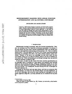
Figure 1. A simple CC network with two inputs and a single output (in gray), and the change in the network as two new nodes are added.

ing a “good” set of basis functions has a very significant and direct effect on the success of the method. As mentioned in Sec. 1, given a problem, it is highly desirable to determine a compact set of such basis functions automatically. In the next section, we will first describe cascade-correlation learning architecture, and then present how they can be utilized in the LSPI algorithm to constuct new basis functions iteratively.

3. Cascade-Correlation Networks Cascade-correlation (CC) is both an architecture and a supervised learning algorithm for artificial neural networks introduced by [2]. It aims to overcome step-size and moving target problems that negatively affect the performance of back-propagation learning algorithm. Instead of having a predefined topology with the weights of the fixed connections between neurons getting adjusted, a CC network starts with a minimal structure consisting only of an input and an output layer, without any hidden layer. All input neurons are directly connected to the output neurons (Fig. 1a). Then, the following steps are taken: 1. All connections leading to output neurons are trained on a sample set and corresponding weights (i.e. only the input weights of output neurons) are determined by using an ordinary learning algorithm (such as “delta” rule, or more efficient methods like RPROP) until the error of the network no longer decreases. Note that, only the input weights of output neurons are being trained, therefore there is no backpropagation. 2. If the accuracy of the network is above a given threshold then the process terminates. 3. Otherwise, a set of candidate units is created. These units typically have non-linear activation functions. Every candidate unit is connected with all input neurons and with all existing hidden neurons (which is initially empty); the weights of these connections are initialized randomly. At this stage the candidate units are not connected to the output neurons, and therefore are not actually active in the network. Let s denote a training sample. The connections leading to a candidate unit are trained with the goal of maximiz-

ing the sum S over all output units o of the magnitude of the correlation between the candidate units value denoted by vs , and the residual error observed neuron o denoted Pat output P by es,o . S is defined as S = o | s (vs − v)(es,o − eo )| where v and eo are the values of vs and es,o averaged over all samples, respectively. As in step 1, learning takes place with an ordinary learning algorithm by performing gradient ascent with respect to each P of the candidate units incoming weights ∂S/∂wi = s,o (es,o − eo )σo fs0 Ii,s where σo is the sign of the correlation between the candidates value and output o, fs0 is the derivative for sample s of the candidate units activation function with respect to the sum of its inputs, and Ii,s is the input the candidate unit received from neuron i for sample s5 . The learning of candidate unit connections stops when the correlation scores no longer improve or after a certain number of passes over the training set. Now, the candidate unit with the maximum correlation is chosen, its incoming weights are frozen (i.e. they are not updated in the subsequent steps) and it is added permanently to the network by connecting it to all output neurons (Fig. 1b and c, solid lines show frozen weights). All other candidate units are discarded. 4. Return back to step 1. Until the desired accuracy is achieved at step 2, or the number of neurons reaches a given maximum limit, a CC network completely self-organizes itself. By adding hidden neurons one at a time and freezing their input weights, training of both the input weights of output neurons (step 1) and the input weights of candidate units (step 3) reduce to one step learning problems. Since there is no error to back-propagate to previous layers the moving target problem is effectively eliminated. Also, by training candidate nodes with different activation functions and choosing the best among them, it is possible to build a more compact network that better fits the training data6 . More importantly, each hidden neuron effectively becomes a basis function in the network; the successive addition of hidden neurons in a cascaded manner allows, and further, facilitates the creation of more complex basis functions that helps to reduce the error and better represent the target function. This entire process is well-matched to our goal of determining a set of good basis functions for function approximation in RL, in particular within the scope of LSPI algorithm. We now describe our approach for realizing this. 5 Note that, since only the input weights of candidate units are being trained there is again no need for back-propagation. Besides, it is also possible to train candidate units in parallel since they are not connected to each other. By training multiple candidate units instead of a single one, different parts of the weight space can be explored simultaneously. This consequently increases the probability of finding neurons that are highly correlated with the residual error. 6 Furthermore, with deterministic activation functions the output of a neuron stays constant for a given sample input; hence, the number of calculations in the network can be reduced by storing the output values of neurons, improving the efficiency compared to traditional networks.

Algorithm 2 LSPI with basis function expansion. ~ init , Require: Set of samples S, initial basis functions φ discount factor γ, number of candidate units n. ~ init | inputs and a single 1: Create a CC network N with |φ output, and set activation functions of input units to φi . ~←φ ~ init 2: φ 3: repeat ~ γ) 4: w ← LSP I(S, φ, 5: Set the weight between ith unit and the output wi . b a) − (r + γ Q(s b 0 , πw (s0 ))) over S. 6: Calculate Q(s, 7: Train n candidate units on N , and choose the one κ having the maximum correlation with the residual error. 8: Add κ to N . ~ . φκ is the function represented by κ. 9: Add φκ to φ 10: until termination condition is satisfied 11: return w and φ

4. Using Cascade-Correlation Learning Architecture in Least-Squares Policy Iteration As described in Sec. 2, in LSPI the state-action value function of a given policy is approximated by a linear combination of basis functions. Our aim here is to employ CC networks as function approximators and at the same time use them to find useful basis functions in LSPI. Given a reinforcement learning problem, suppose that we have a set of state-action basis functions Φ = {φ1 (s, a), φ2 (s, a), . . . , φm (s, a)}. Using this basis functions and applying LSPI algorithm on a set of collected samples of the form (s, a, r, s0 ), we can find a set of parameters wi together with an approximate state-action value function b a) = Pm wi φi (s, a) and derive a policy π Q(s, b which i=1 b Let N be a CC network with is greedy with respect to Q. m inputs and a single output having linear activation function (i.e. identity function). In this case, the output of the network is a linear combination of the activation values of input and hidden neurons of the network weighted by their connection weights. Initially, the network does not have any hidden neurons and all input neurons are directly connected to the output neuron. Therefore, by setting the activation function of the ith input neuron to φi and the weight of its connection to the output neuron to wi , N becomes funcb and outputs Q(s, b a) when all input tionally equivalent to Q neurons receive the (s, a) tuple as their input. Now, the Bellman operator Tπ is known to be a contraction in L∞ norm, that is for any state-action value function Q, Tπ Q is closer to Qπ in the L∞ norm, and in particular as mentioned in Sec. 2, Qπ is a fixed point of Tπ . Ideally, a good approximation would be close to its image under the Bellman operator. As opposed to the Bellman residual minimizing approximation, least-squares fixed-point approxi-

mation, which is at the core of the LSPI algorithm, ignores b and Q b but rather focuses on the the distance between Tπb Q direction of the change. Note that, if the true state-action value function Qπ lies in the subspace spanned by the basis functions, that is the set of basis functions is “rich” enough, fixed-point approximation would be solving the Bellman equation and the solution would also minimize the magnitude of the change. This hints that, within the scope of LSPI, one possible way to drive the search towards solutions that satisfy this property could be to expand the set of basis functions by adding new basis functions that are likely to reduce the distance between the found state-action b and Tπb Q b over the sample set. For this value function Q purpose, given a sample (s, a, r, s0 ), in the CC network we b 0, π can set r + γ Q(s b(s0 )) as the target value for (s, a) tuple, and train candidate units that are highly correlated with the b a) − (r + γ Q(s b 0, π residual output error, that is Q(s, b(s0 ))). At the end of the training phase, the candidate unit having the maximum correlation is added to the network by transforming it into a hidden neuron, and becomes the new basis function φm+1 ; φm+1 (s, a) can be calculated by feeding (s, a) as input to the network and determining the activation value of the hidden neuron. Through another round of LSPI learning, one can obtain a new least-squares fixed-point approximation to the state-action value function b 0 (s, a) = Pm+1 w0 φi (s, a) which is more likely to be a Q i i=1 better approximation also in the sense of Bellman residual minimization. The network is then updated by setting the weights of connections leading to the output neuron to wi0 for each basis function. This process can be repeated, introducing a new basis function at each iteration, until the error falls below a certain threshold, or a policy with adequate performance is obtained. We can regard this as a hybrid learning system, in which the weights of connections leading to the output neuron of the CC network are being regulated by the LSPI algorithm. Note that, the values of all basis functions for a given (s, a) tuple can be found with a feed-forward run over the network.The complete algorithm that incorporates the CC network and basis function expansion to LSPI is presented in Algorithm 2 7 . In the proposed method, LSPI is run to completion at each iteration, and then a new basis function is generated using the cascade correlation training. This benefits from a more accurate approximation of the state-action value function for the current set of basis functions. An alternative approach would be to add new basis functions within the LSPI loop after the policy evaluation step (i.e. after each or several calls to LSTDQ). For situations in which LSPI 7 One possible problem with the proposed method is that, especially when the sample set is small, with increasingly complex basis functions there may be over-fitting. This can be avoided by increasing the amount of samples, or alternatively a cross-validation approach can be ensued by applying LSPI algorithm independently on multiple sample sets but training a single set of candidate units over all sample sets.

Algorithm 3 Within loop variant of Algorithm 2. ~ initial , Require: Set of samples S, initial basis functions φ discount factor γ, number of candidate units n. ~ γ, w0 ) 1: function LSPI(S, φ, ~ inputs and a single 2: Create a CC network N with |φ| output, and set activation functions of input units to φi . 3: w ~ 0 ← initial weights 4: repeat . Update the policy until it converges. ~ γ, πw ) 5: w ~ i ← LSTDQ(S, φ, i−1 6: Run steps 5-10 of Algorithm 2. 7: Add a new weight to w ~i corresponding to the new basis function φκ . 8: until (kwi − wi−1 k <  and residual error is small) or i > imax ~ 9: return wi and φ 10: end function requires a relatively large number of iterations to converge, this within loop variant of the algorithm, as presented in Algorithm 3, may lead to better intermediate value functions and steadier progress towards the optimal solution; since some of the policy evaluation steps may be discarded, it can also potentially be more efficient. However, the resulting basis functions may not be useful at later iterations and more basis functions may be required to achieve the desired performance level. Finally, we would like to note that one can also combine these two approaches by first adding new basis functions temporarily within the LSPI loop, using the resulting state-value function to calculate the residual error in Algorithm 2 and add a new permanent basis function, and then discarding the temporary ones.

5. Experiments We have evaluated the proposed method on three problems: chain walk [7], pendulum swing-up and multisegment swimmer8 In all problems, we started from a set of basis functions consisting of: (i) a constant bias, (ii) a basis function for each state variable, which returns the normalized value of that variable, and (iii) a basis function for each possible value of each control variable, which returns 1 if the corresponding control variable in the state8 Chain walk is an MDP consisting of a chain of n states. There are c two actions, lef t and right, which succeed with probability 0.9, or else fail, moving to the state in the opposite direction. The first and last states are dead-ends, i.e. going left at the first state, or right at the last state revert back to the same state. The reward is 1 if an action ends up in a predefined set of states, and 0 otherwise. The pendulum swing-up and multi-segment swimmer problems are dynamical systems where the state is defined by the position and velocity of the elements of the system, and actions (applied forces) define the next state: these are non-linear control tasks with continuous state spaces. We refer the reader to [1] for a complete specification of both inverted pendulum and swimmer problems. In the sequel, we denote ns the number of segments of the swimmer.

6 5 4 3 2 1 6 5 4 3 2 1 6 5 4 3 2 1 0

10

20

30

40

50

10

20

30

40

10

20

30

40

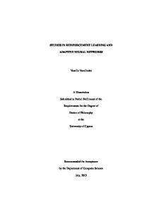
Figure 2. Q-functions for the 50-state chain problem with 5, 10 and 20 basis functions (left to right). See text for description.

action tuple is equal to that value, and 0 otherwise. In the LSPI algorithm, we set  = 10−4 and limit the number of iterations to 20. The samples for each problem are collected by running a random policy, which uniformly selects one of possible actions, for a certain number of time steps (or episodes). In CC network, we trained an equal number of candidate units having Gaussian and sigmoid activation functions using RPROP method [13]9 . We allowed at most 100 passes over the sample set during the training of candidate units, and employed the following parameters: 4min = 0.0001, 4ini = 0.01, 4max = 0.5, η − = 0.5, η + = 1.2. Figure 2 shows the results for the 50-states (numbered from 0 to 49) chain problem using 5000 samples from a single trajectory. Reward is given only in states 9 and 40, therefore the optimal policy is to go right in states 0-8 and 25-40, and left in states 9-24 and 41-49. The number of candidate units was 4. In [7], using 104 samples LSPI fails to converge to the optimal policy with polynomial basis function of degree 4 for each action, due to the limited representational capability, but succeeds with a radial basis function approximator having 22 basis functions. Solid lines denote action “left” and dashed lines denote action “right”. LSPI is run to completion (bottom), a basis function is added after each (middle), or after every two LSTDQ calls (top). Using cascade-correlation basis expansion, optimal policies can be obtained within 10 basis functions, and accuracy of the state-action value approximation increases with additional ones. In this and other problems that we analyzed, LSPI 9 In

RPROP, instead of directly relying on the magnitude of the gradient for the updates, each parameter is updated in the direction of the corresponding partial derivative with an individual time-varying value that depends on the change in the sign of the partial derivatives.

avg. total reward

140 120 100 80 60 40 20 0 -20 -40 -60

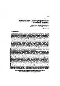
basis functions in case of 5000 and 10000 samples, respectively). We observed a similar behavior on more complex 5-segment swimmer problem as presented in Fig. 3b. For this problem, we collected 100000 samples restarting from a random configuration every 50 time steps. The number of trained candidate units was 10 as in the pendulum problem, but we allowed RPROP to make a maximum of 200 passes over the sample set as the problem is more complex.

rbf (5000 samples) rbf (10000 samples) 5000 samples 10000 samples 5

10

15

20 25 30 35 40 # of basis functions

45

50

55

6. Related Work

(a) 10

avg. reward

5 0 -5 -10 -15 -20 -25 0

5

10

15 iteration

20

25

30

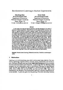
(b) Figure 3. The progress of learned policies after each new basis function in the (a) pendulum and (b) 5 segment swimmer problems.

tends to converge in small (2-4) number of iterations. This is probably due to the fact that the number of initial basis functions does not need to be large and policies are reused after each basis function expansion. Therefore, both Algorithm 2 and its within loop variant Algorithm 3 perform similar. The basis functions start from simpler ones and get more complex in order to better fit the target function. The results for the pendulum problem are presented in Fig. 3a. For this problem, we collected two sets of samples of size 5000 and 10000, restarting from a random configuration every 20 time steps, and trained 10 candidate units. For both data sets, we also run LSPI using a radial basis function approximator on a 16 × 16 regular grid for each action. This corresponds to a set of 514 basis functions, including two bias terms. We averaged over 30 different runs. As it can be clearly seen from Fig. 3, with less number of samples the performance of policies obtained by radial basis function approximator decrease drastically. On the other hand, for both cases, the performance of the policies found by LSPI algorithm using the discovered basis functions converge to the same level. We also observe a consistent improvement as new basis functions are added (except in the very first iterations), yielding better performance levels using much less number of basis functions (10 and about 20

Basis function, or feature selection and generation is essentially an information transformation problem; the input data is converted into another form that “better” describes the underlying concept and relationships, and “easier” to process by the agent. As such, it can be applied as a preprocessing step to a wide range of problems and recently attracted attention from the RL community. In [10], Menache et al. examined adapting parameters of a set of Gaussian radial basis functions for estimating the value function of a fixed policy. In particular, for a given set of parameters, they used LST D(λ) to determine the weights of basis functions that approximate the value function of a fixed control policy, and then applied either a local gradient based approach or global cross-entropy method to tune the parameters in order to minimize the Bellman approximation error in a batch manner. The results of experiments on a grid world problem show that cross-entropy based method performs better. In [6], Keller et al. studied automatic basis function construction for value function approximation within the context of LSTD. Given a set of trajectories and starting from an initial approximation, they iteratively use neighborhood component analysis to find a mapping from the state space to a low-dimensional space based on the estimation of the Bellman error, and then by discretizing this space aggregate states and use the resulting aggregation matrix to derive additional basis functions. This tends to aggregate states that are close to each other with respect to the Bellman error, leading to a better approximation by incorporating the corresponding basis functions. In [11], Parr et al. showed that for linear fixed point methods, iteratively adding basis functions such that each new basis function is the Bellman error of the value function represented by the current set of basis functions forms an orthonormal basis with guaranteed improvement in the quality of the approximation. However, this requires all computations be exact, that is, are made with respect to the precise representation of the underlying MDP. They also provide conditions for the approximate case, where progress can be ensured for basis functions that are sufficiently close to the exact ones. Their application in the approximate case on LSPI is closely related to our work, but differs in the sense that a new basis function for each action

is added at each policy-evaluation phase by directly using locally weighted regression to approximate the Bellman error of the current solution. In contrast to these approaches that make use of the approximation of the Bellman error, including ours, the work by Mahadevan et al. aims to find policy and reward function independent basis functions that captures the intrinsic domain structure that can be used to represent any value function [5, 9]. Their approach originates from the idea of using manifolds to model the topology of the state space; a state space connectivity graph is built using the samples of state transitions, and then eigenvectors of the (directed) graph Laplacian with the smallest eigenvalues are used as basis functions. These eigenvectors possess the property of being the smoothest functions defined over the graph and also capture the nonlinearities in the domain, which makes them suitable for representing smooth value functions. To the best of our knowledge, the use of CC networks in reinforcement learning has rarely been investigated before. One existing work that we would like to mention is by Rivest and Precup (2003), in which CC network purely functions as a cache and an approximator of the value function, trained periodically at a slower scale using the state-value tuples stored in the lookup-table [14]. Finally, we are currently investigating various tracks in our own team. In particular, we would like to mention the use of genetic programming to build useful basis functions [4]. Using a genetic programming approach opens the possibility to obtain human-understandable functions. We also investigate a kernelized version of the LARS algorithm [8]. This basically selects the set of best basis functions to represent a given function, according to set of sample data points; they are automatically generated as in any kernel method.

7. Conclusion In this paper, we explored a new method that combines CC learning architecture with least-squares policy iteration algorithm to find a set of basis functions that would lead to a better approximation of the state-action value function, and consequently results in policies with better performance. The experimental results indicate that it is effective in discovering such functions. An important property of the proposed method is that the basis function generation process requires little intervention and tuning from the user. We believe that learning sparse representations is a very important issue to tackle large reinforcement learning problems. A lot of work is still due to get a proper, principled approach to achieve this, not mentioning the theoretical issues that are pending. Among on-going work, the way LSPI and the basis function construction process are intertwined needs more work. Although, our focus was on LSPI algorithm in this paper, the approach is neither restricted to LSPI, nor value-based reinforcement learning; [3] demon-

strates that the same kind of approach may be embedded in natural actor-critics. In particular, Sigma-Point Policy Iteration (SPPI) and fitted Q-learning may be considered, SPPI being closely related to LSPI, and fitted Q-learning having demonstrated excellent performance and having nice theoretical properties. We pursue future work in this direction and also apply the method to more complex domains.

References [1] R. Coulom. Reinforcement Learning Using Neural Networks with Applications to Motor Control. PhD thesis, Institut National Polytechnique de Grenoble, 2002. [2] S. E. Fahlman and C. Lebiere. The cascade-correlation learning architecture. In D. S. Touretzky, editor, Advances in NIPS, volume 2, pages 524–532. Morgan Kaufmann, 1990. [3] S. Girgin and P. Preux. Basis expansion in natural actor critic methods. In Proc. of the 8th European Workshop on Reinforcement Learning, June 2008. [4] S. Girgin and P. Preux. Feature discovery in reinforcement learning using genetic programming. In Proc. of Euro-GP, pages 218–229. Springer-Verlag, Mar. 2008. [5] J. Johns and S. Mahadevan. Constructing basis functions from directed graphs for value function approximation. In ICML, pages 385–392, NY, USA, 2007. ACM. [6] P. W. Keller, S. Mannor, and D. Precup. Automatic basis function construction for approximate dynamic programming and reinforcement learning. In ICML, pages 449–456, NY, USA, 2006. ACM. [7] M. G. Lagoudakis and R. Parr. Least-squares policy iteration. J. of Machine Learning Research, 4:1107–1149, 2003. [8] M. Loth, M. Davy, and P. Preux. Sparse temporal difference learning using LASSO. In Proc. of the IEEE International Symposium on Approximate Dynamic Programming and Reinforcement Learning, Apr. 2007. [9] S. Mahadevan and M. Maggioni. Proto-value functions: A laplacian framework for learning representation and control in markov decision processes. J. of Machine Learning Research, 8:2169–2231, 2007. [10] I. Menache, S. Mannor, and N. Shimkin. Basis function adaptation in temporal difference reinforcement learning. Annals of Operations Research, 134:215–238(24), 2005. [11] R. Parr, C. Painter-Wakefield, L. Li, and M. Littman. Analyzing feature generation for value-function approximation. In ICML, pages 737–744, NY, USA, 2007. ACM. [12] M. Puterman. Markov Decision Processes — Discrete Stochastic Dynamic Programming. Probability and mathematical statistics. Wiley, 1994. [13] M. Riedmiller and H. Braun. A direct adaptive method for faster backpropagation learning: the rprop algorithm. pages 586–591 vol.1, 1993. [14] F. Rivest and D. Precup. Combining td-learning with cascade-correlation networks. In T. Fawcett and N. Mishra, editors, ICML, pages 632–639. AAAI Press, 2003. [15] R. S. Sutton and A. G. Barto. Reinforcement Learning: An Introduction. MIT Press, Cambridge, MA, 1998. A Bradford Book.