coefficients of basis functions has a unique solution (Bartels et. al. ...... Hagen, Hans (September 1985) \Geometric Spline Curves," Computer Aided Geometric.
Basis Functions for Rational Continuity Dinesh Manocha1 Brian A. Barsky2 Computer Science Division University of California at Berkeley Berkeley, California 94720
Abstract:
The parametric or geometric continuity of a rational polynomial curve has often been obtained by requiring the homogeneous polynomial curve associated with the rational curve to possess parametric or geometric continuity, respectively. Recently this approach has been shown overly restrictive. We make use of the necessary and su�cient conditions of rational parametric continuity for de ning basis functions for the homogeneous representation of a rational curve. These functions are represented in terms of shape parameters of rational continuity, which are introduced due to these exact conditions. The shape parameters may be varied globally, a�ecting the entire curve, or modi ed locally thereby a�ecting only a few segments. Moreover, the local parameters can be represented as continuous or discrete functions. Based on these properties, we introduce three classes of basis functions which can be used for the homogeneous representation of rational parametric curves.
Keywords:
Rational Curves, Parametric Continuity, Geometric Continuity, Shape Parameters, Splines
Supported by Alfred and Chella D. Moore Fellowship. Supported in part by a National Science Foundation Presidential Young Investigator Award (number CCR-8451997) 1 2
1 Introduction The rational formulation of polynomials and splines has received considerable interest in the areas of computer graphics and geometric modeling. The main advantage of the rational form is its ability to represent conic curves and quadric surfaces, as well as free-form curves and surfaces (Piegl 1985; Piegl 1986a; Piegl 1986b; Piegl 1986c; Piegl and Tiller 1987; Salmon 1879; Tiller 1983; Versprille 1975). Moreover, it is invariant under a�ne as well as projective transformations, though the latter is possible with changed weights (Lee 1987). A single rational polynomial usually does not have enough freedom to represent a given curve; several rational polynomial segments are used instead. To obtain a curve of satisfactory smoothness, the segments must connect with some amount of continuity. Thus, the use of rational curves, independent of the particular variety, creates the problem of connecting rational polynomial segments to form piecewise rational curves that are smooth. To obtain rational curves with either parametric or geometric continuity, the parametric continuity constraints or geometric continuity constraints, respectively, have been applied to the components of the curve in homogeneous coordinates, but not to the components of the rational curve (Barsky 1988a; Boehm 1987; Farin 1983; Goldman and Barsky 1989a; Goldman and Barsky 1989b; Joe 1989; Tiller 1983). If the homogeneous curve satis es the relevant continuity constraints then the rational curve will have the corresponding continuity. There are two kinds of continuity for parametric curves: parametric continuity and geometric (or visual) continuity. A curve is said to possess parametric continuity (denoted C n ) if each segment of the curve is C n and the adjacent segments are connected with C n continuity at the joints. There are two notions of geometric continuity. The rst is based on parametric continuity after a suitable reparametrization. That is, a curve is said to be geometrically continuous (denoted Gn ) if there exists some reparametrization of its segments such that the resulting curve is C n . The reparametrization criterion on its segments leads to the derivation of Beta-constraints (Barsky 1988b; Barsky and DeRose 1989; Barsky and DeRose 1990; DeRose 1985). The second notion of geometric continuity of parametric curves is based on the continuity of Frenet Frame and higher order curvatures (Boehm 1985; Boehm 1987; Dyn and Micchelli 1985; Hagen 1985). A curve possesses geometric continuity Gn if each of its components satis es the corresponding constraints at the joints. However, these constraints are su�cient but not necessary for the continuity of rational curves (Hohmeyer and Barsky 1989). The necessary and su�cient constraints for rational continuity (parametric or geometric continuity), as applied to the homogeneous curve, give rise to shape parameters. These shape parameters are di�erent from and in addition to those obtained from the geometric continuity of polynomial or rational curves and surfaces (dubbed as Betas). They are used for modifying the curve independent of the control vertices. Experience has shown us that shape parameters provide a designer with intuitive control of shape. Some of the properties of these parameters are very useful for the 1
development of modern geometric modeling system. In this paper, we introduce three categories of basis functions for the homogeneous representation of rational curves. These basis functions are based upon the necessary and su�cient conditions for rational parametric continuity. The di�erent categories are obtained by varying the shape parameters globally, which a�ects the entire curve, or locally, which a�ects only a few segments only. For the local variation, the shape parameters may be either continuously varying functions or be discretely speci ed at the knot values. The resulting basis functions di�er in the amount of local control (with respect to shape parameters) and evaluation cost. The rest of the paper is organized in the following manner: In Section 2, we give a brief overview of rational curves and specify the notation. The necessary and su�cient conditions for the parametric continuity of rational curves are mentioned in Section 3. They are used in Section 4 for de ning the basis functions for the homogeneous representation of rational curves with uniform shape parameters. In Section 5, the uniform shape parameters are generalized into continuously varying shape parameters by quintic Hermite interpolation. Section 6 speci es a discretely-shaped homogeneous basis. Finally, in Section 7 we present the formulation which can be used for constructing rational curves satisfying the necessary and su�cient conditions for geometric continuity. 3
2 Rational Curves A rational polynomial function is a scalar function, r : R ! R that can be expressed as r(u) = fg((uu)) where f(u) and g(u) are polynomials in u. We will restrict our use of the word polynomial in the following manner: a rational function is not a polynomial function unless its denominator divides its numerator. Such a function is at times referred to as an integral function to distinguish it from a rational function. A curve is simply a vector-valued function q : R ! Rd. A rational curve is a vector-valued function, each component of which is a rational function. There are at least two ways to represent a rational curve (Hohmeyer and Barsky 1989). First, the curve q(u) can be thought of as a vector-valued function, each component of which is a rational function. Alternatively, q(u) can be thought of as a vectorvalued function Q : R ! Rd with a projection function that projects (x ; : : :; xd; xd ) to (x =xd ; : : :; xd=xd ). That is, the function is originally in (d + 1 )-dimensional space but is then projected down to a d-dimensional space. +1
1
+1
1
+1
+1
Any homogeneous representation of a xed degree will be a linear combination of these functions. However, they do not form any basis spanning a vector space, since the rational curves of a xed degree do not constitute a vector space. 3
2
In the rst representation, we write:
q(u) = (r (u); r (u); : : :; rd(u)) 1
2
where each component function, ri(u), is a rational function of the form fg uu . In the second representation, one might consider the same curve as a polynomial curve whose range is the homogeneous coordinate system of dimension d +1. The rational curve q(u), discussed above, would be represented in this scheme by the polynomial curve Q(u), where i(
) ( )
Q(u) = (f (u); : : :; fd(u); g(u)) 1
which is in (d + 1)-dimensional space. We refer to Q(u) as the homogeneous curve associated with q(u), the rational curve or the projected curve, and q(u) as the projection of Q(u). The homogeneous curve is not unique, whereas the projection is. Moreover, we use italics to indicate scalar-valued functions, such as f (u ) or g (u ), boldface lower case to indicate vector-valued rational curves, such as q(u), whose range is Rd , and bold face upper case to indicate the associated homogeneous polynomial curve, such as Q(u), whose range is Rd . The degree of a rational curve is the degree of its homogeneous representation. To illustrate more concretely, consider a curve formulation such as the rational B�ezier curve, the rational B-spline curve, or the rational Beta-spline curve of a xed degree. Each is a function q : R ! Rd that can be expressed as m (1) q(u) = X Vi [ PmwiBwi(Bu)(u) ] j j j i +1
=0
=0
where Vi 2 Rd are the control vertices, Bi(u) are the basis functions for the homogeneous curve, de ned as a polynomial curve, and wi are the weights, for i = 0; : : : ; m, which are independent of the control vertices and the basis functions. One can also consider such a curve as a polynomial B�ezier curve, B-spline curve, or Beta-spline curve in the homogeneous space: m X Q(u) = WiBi(u)
i=0 d +1 where i are control vertices in R , whose coordinates are expressed as i = (wi i; wi) for i = 0; : : :; m. Whenever the Rd coordinates of (u) are required, the division must be
W
q
W
V
performed. For example, the circle in Fig. I is a rational curve in R , which is a projection of a polynomial curve in R . The points on the R curve are obtained by projecting the R curve onto the w = 1 plane. The advantage of this perspective is that the algorithms to manipulate rational curves (i.e. evaluation, subdivision, degree elevation etc.) can be obtained by using the corresponding algorithm for polynomial curves. This method of reducing a problem associated with a rational curve to the analogous problem for its homogeneous counterpart has also 2+1
2
2+1
3
2
been used for the problem of continuity, parametric or geometric, between rational segments. It is true that if the homogeneous curve satis es the relevant continuity constraints then the rational curve will have the corresponding continuity. However, there are cases when the projected curve satis es the required continuity constraints, whereas the corresponding homogeneous curve does not (Hohmeyer and Barsky 1989). Thus, the above approach is overly restrictive. One such case is shown in Fig. I. A circle is being generated with C rational curves. In the gure, the circle has been shown as a projection of a homogeneous curve, Q(u) 2 R , onto the w = 1 plane. The axis of the cone (whose base is also shown) lies along the w-axis. The tip is at the origin and the homogeneous curve Q(u) consists of four segments, lying on the surface (including the base) of the cone and it is C continuous. Q(u) is neither C nor even G , whereas q(u) is trivially C . The necessary and su�cient constraints on the homogeneous curve engenders shape parameters (Hohmeyer and Barsky 1989). The basis functions for the homogeneous representation, Bi(u), as speci ed in (1), become functions of these shape parameters. Changing the shape parameters changes the projected curve, while still satisfying the necessary conQ tinuity constraints. 0
2+1
0
1
1
2
w y
q
w = 1 plane
x
Fig. I A circle q(u) represented by a piecewise rational Q(u). There are kinks in Q(u), but q(u) is C continuous. 2
3 Continuity Constraints In our case the smoothness of a curve has been measured by testing the parametric continuity of the functions de ning the curve. If we have a homogeneous curve Q(u) that is C n, then the projection q(u) of Q(u) will also be C n . However, the converse is not true. As mentioned earlier, there are homogeneous curves Q(u) that are not C n even though 4
their projections q(u) are C n . The curve q(u) is C n , say at u = u , if and only if each component of q(u), which is of the form fi(u)=g (u), is C n at u = u . Consider a generic quotient function of the type f (u)=g(u). The necessary and su�cient conditions so that such a quotient function would be C n at a point u = u are that there exist �i's such that 0
0
0
2 66 66 lim 6 u!u0 + 6 64
3
2
3
2
3
f (u) 7 6 � 0 0 ::: 0 07 66 ff ((uu)) 77 f (u) 77 66 � � 0 ::: 0 0 77 6 7 � ::: 0 0 77 lim 66 f (u) 77 (2) f (u) 777 = 666 � 2� 77 ... ... ... ... 77u!u0 ;66 ... ... 75 64 ... ::: 5 4 5 �n (n)�n; (n )�n; : : : (nn; )� � f n (u) f n (u) and similarly for the function g(u) (with the same set of �i's). At any point u = u , all the functions fi(u) and g(u) need to satisfy the above relation for any set of �'s where � 6= 0 (Hohmeyer and Barsky 1989). In other words, each component of Q(u) is related by the above constraint at each knot value and the set of �'s must be the same for all components. We use the �'s de ned above as shape parameters. Changing the values of the �'s gives a di�erent projected curve q(u), which maintains the desired continuity. In most computer graphics applications, cubic curves are used because they provide a balance between computational cost and the desired smoothness and exibility. The desired smoothness is frequently ensured by requiring the curve to be C continuous in the desired interval. So we formulate a cubic basis for the homogeneous curve and generate a C projected curve q(u). Thus, there are three shape parameters, � ; � , and � , that determine our projected curve q(u). For this case, (2) can be rewritten in the following manner (n=2): 2 3 2 3 2 3 f (u) � 0 0 f (u) 64 f (u) 75 = 64 � � 0 75 lim 64 f (u) 75 lim (3) u!u0 u!u0 ; � 2 � � f (u) f (u) (0) (1)
0 1
(2)
( )
(1)
0
2
1
1
(0)
(2)
0
1
2
2
1
1
( )
0
0
0
2
2
0
(0) (1)
+
(2)
1
2
(0)
0 1
(1)
0
2
1
0
(2)
We will initially use �'s as uniform shape parameters. That is, each shape parameter has the same value at the knots. We later generalize them to continuous functions of shape parameters, where the user is not constrained to use the same value and it o�ers maximum local control of these parameters. The latter formulation turns out to be computationally expensive. Therefore, at the end we introduce a discretely-shaped basis for the homogeneous curve, which provides a balance between evaluation cost and the degree of local control of shape parameters. For each case, we will de ne a basis function and use (1) to determine the projected curve q(u).
4 Uniform Shape Parameters In this section, we de ne the basis functions for the homogeneous curve. Our terminology is similar to that described in (Bartels et. al. 1987, Chapter 2). The rational curve is 5
obtained by projecting the linear combinations of the basis functions. The scalar multiples used for the linear combinations are determined by the control vertices and weights. The representation of a rational curve q(u), as de ned in (1), leads to the formation of the following functions: (4) Ri(u) = PmwiBwi(Bu)(u) ; i = 0; : : : ; m j =0 j j
where the Bj (u) are the basis functions for the homogeneous curve. The resulting curve q(u) must be C continuous in the speci ed interval. The desired continuity could be achieved if Ri(u) were themselves C functions, since the rational curve is a linear combination of these functions. This happens if each Bj (u) and its rst two derivatives are related by (3) at ui. To simplify, we work over a uniform knot sequence and derive the canonical basis function in a manner similar to that described in (Bartels et. al. 1987). 2
2
4.1 The Basis Functions Each Bi (u) consists of four basis segments. We denote these segments by bi(u); i = 0; 1; 2; 3. Each segment is a cubic polynomial of the form
u 2 [0; 1) i = 0; 1; 2; 3
bi(u) = pi + qiu + riu + siu ; 2
3
At the knot values, the Bj (u) are related by (3). This engenders the following fteen relations among the bi (u): 0 � b (1) � b (1) � b (1) � b (1) 0 0
0 1
0 2
0 3
= = = = =
b (0); b (0); b (0); b (0); 0; 0 1
2
3
0 � b (1) + � b (1) � b (1) + � b (1) � b (1) + � b (1) � b (1) + � b (1)
= = = = =
1 0 0 1 0 1 1 0 2 1 0 3
1 0
1 1
1 2
1 3
b (0); b (0); b (0); b (0); 0;
0 � b (1) + 2� b (1) + � b (1) � b (1) + 2� b (1) + � b (1) � b (1) + 2� b (1) + � b (1) � b (1) + 2� b (1) + � b (1)
1 0 1 1 1 2 1 3
1 1 0 1 1 1 1 1 2 1 1 3
2 0
2 1
2 2
2 3
2 0 0 2 0 1 2 0 2 2 0 3
= = = = =
b (0) b (0) b (0) b (0) 0 2 0 2 1 2 2 2 3
There are four cubic functions, b (u); b (u); b (u) and b (u), which constitute Bj (u). Each has four unknowns (equal to the order of each polynomial). Thus, there are sixteen variables in all. Any sixteen independent variables, each being de ned over the real eld R, belong to the 16-dimensional vector space R . In our case, the variables are not independent. On applying the fteen constraints we obtain a 1-dimensional subspace of the 16-dimensional vector space. Geometrically, the fteen constraints given above determine a line in the 16-dimensional space. Moreover, that line passes through the origin (as it is a vector subspace). Any point lying on that line, except the origin, would determine a solution set to the sixteen variables. That solution set is of the following form: 0
1
2
3
16
[s g; s g; : : : ; s g; s g]T 1
2
15
where each si is a function of � , � , and � . 0
1
2
6
16
The variable g acts as a normalizing factor. If g = 0 then the basis function Bj (u) becomes equal to a zero function (it is zero throughout). We let bi (u) be de ned in terms of g. The rational basis functions Ri(u) are independent of g, as it cancels out in the numerator and denominator terms of (4), since g 6= 0. In the case of polynomial B-splines and Beta-splines, formed from C and G continuity constraints, respectively, the fact that the basis functions should form a partition of unity gives rise to the sixteenth constraint and the system of equations used for determining the coe�cients of basis functions has a unique solution (Bartels et. al. 1987). The fact that Ri(u); i = 0; : : : ; m, should form a partition of unity is embedded in their formulation and no such constraint is required on Bi(u). That property engenders another shape parameter, expressed above as g. If we use a di�erent value of g for each Bi(u), then it has a local e�ect on the curve. The e�ect is similar to that of the weights for rational curves expressed as (1). However, the weights are present due to the homogeneous representation of the vertices; i.e., Wi = (wiVi ; wi). If we want to use these basis functions for homogeneous representations of tensor product surfaces, the g's will a�ect the surface in a di�erent manner as compared to the weights. Using Macsyma (Fateman 1982), we obtain the following basis functions for the homogeneous representation of the rational curve: b (u) = gu b (u) = g (� + [� + 3� ]u + [ � + 6�2 + 6� ]u ; [ � + 6�2 + 6� ]u ) b (u) = g ([� � + 4� ] + [ � (4� ; �2 ) + 2� ]u + (5) [� (� ; 6� ) ; 2� ; 6� ]u + [ � (6� ; � )2+ 2� + 6� u ]) b (u) = g� (1 ; 3u + 3u ; u ) 2
2
4
3
0 1
0
2
1
0
0
2
0
2 0
1
2
1
1
2 1
1
3 0
3
2
0
0
2
1
0
3
2 1
2
2 0
2
2
0
1
2 1
2
2 0
3
3
If we set
� = 1; � = 0; � = 0 then the above basis reduces to a basis for the uniform cubic B-spline (Bartels et. al. 1987). These are the default values of the shape parameters and the resulting function is a basis for the homogeneous representation of a cubic rational B-spline with uniform knot spacing. To determine a curve, we select a set of control vertices Vi and use (1) to de ne the curve. The Bi (u) used in the de nition of Ri(u) in (4) are de ned in terms of the segments bi(u) (5). Each Bi(u) is nonzero over four successive intervals only, say from ui to ui . Thus, over the knot interval [ui ; ui ), the portion of the curve de ning q(u) can be represented as (6) Si(u) = Vi wib (uw) i+b (Vui) +wwi i bb(u(u) )++Vwi i wbi (ub) +(uw) +i Vb i(uw) i b (u) 0
1
2
+4
+3
+4
3
+1
3
+1 2
+2
+1 2
+2 1
+2 1
+3
+3 0
+3 0
This is one of the many of formulations of the basis functions. We can let g be a function of the �'s. We tried many combinations and this is the simplest we could achieve in terms of the size of the coe�cients. 4
7
The whole curve q(u) is composed of m ; 2 segments, Si (u); i = 0; : : :; m ; 3. It is also desirable for the resulting curve q(u) obtained from (1) to lie in the convex hull of the control vertices Vi. Using (4), q(u) can be expressed as
q(u) = X ViRi(u): m
(7)
i=0
Since we are considering a uniform knot sequence, all these relations are de ned for u 2 [0; 1). From the de nition of Ri(u) in (4), we know that: m X i=0
Ri(u) = 1
The only other condition that needs to be satis ed for the convex hull property is
Ri(u) � 0;
u 2 [0; 1);
i = 0; : : : ; m
(8)
A su�cient condition for the above inequality may be obtained by non-negative values of � , � , and � . Large positive values of � result in the loss of convex hull property. Each segment of q(u) lies in the convex hull of the four vertices used for de ning it (6). 0
1
2
2
4.2 Varying the �'s Varying the �'s changes the rational curve. A detailed analysis and explanation of their behavior can be found in (Manocha and Barsky 1990). The shape parameters � and � are found to behave very similar to the bias and tension parameters, and , respectively, of the polynomial and rational Beta-spline curves (Barsky 1988b; Barsky and Beatty 1983; Barsky and DeRose 1989; Barsky and DeRose 1990; DeRose 1985). The planar rational curves resulting from di�erent values of � and � have been shown in Fig. II and Fig. III respectively. Some negative values lead to the occurrence of loops or self-intersections. The positions where adjacent segments meet, called joints, of the rational curve are invariant with respect to altering � (as shown in Fig. IV). 0
1
0
1
2
8
2
1
V1
V0
V2
α = 0.1 0
V3
α = 0 1
V5
V1
V4
V0
α = 0 2
V2
V2
V
0
V
3
α = 2
α = 0
0
1
V4
α = 0
α = 0
1
2
α = 0
1
2
V5
V1
V
V
4
V3
V4
α = 0
0
α = 0
V5
V5
V3
α = 1 0
V1
α = 0.5 0
V1
V0
V2
2
V2
V5
V
α = 10 0
V
3
4
α = 0
α = 0
1
2
Fig. II The shape of the rational curves corresponding to di�erent values of � . 0
V 1
V 0
V 2
α0= 1
V 1
V 0
α1= -3 V 2
α0= 1
V 1
V 0
V 3
V 3
α1= 0 V 2
α0= 1
V 3
α1= 5
V 5
V 1
V 4
V 0
V 5
V 1
V 4
V 0
V 5
V 1
V 4
V 0
α2= 0
α2= 0
α2= 0
V 2
α0= 1
V 5
V 3
α1= -1 V 2
α0= 1
V 5
V 3
V 4
α1= 1
α2= 0
V 2
α0= 1
V 5
V 3
α1= 20
Fig. III Di�erent rational curves corresponding to di�erent values of � . 1
9
V 4
α2= 0
V 4
α2= 0
V
V
1
V
2
5
α = -20 2
α = -10 2
α =0 2
α = 10 2
α = 20 2
α = 30 2
V
V
0
V
3
4
α =1
α =0
0
1
Fig. IV The shape of the rational curves corresponding to di�erent values of � . 2
5 Continuous Shape Parameters In the previous sections the formation and usage of basis functions, have been based on the fact that the �'s are uniform shape parameters; i.e., each parameter assumes a unique value. In this section, they are generalized to continuous shape parameters (though we address them as continuous functions of shape parameters, hereafter) each varying continuously along the curve. The continuous analogues of � , � , and � will be denoted by � (u), � (u), and � (u), respectively, and describe the value of each shape parameter along the curve segment SSi(u); i = 0; : : :; m. SSi(u) represents a segment of the rational curve based on continuous function of shape parameters. Its formulation is similar to Si(u) in (6), except that bi(u) is replaced by bbi(u) (described below). This generalization enables the user to have more precise control over the shape of the curve. The user is no longer constrained to choose a unique value for each shape parameter over the entire curve. The di�erent values of the shape parameters can be used to re ect the local character of the shape parameters along the curve. This is in addition to local control, which is available with respect to the control vertices. For simplicity, we again choose to use a uniform knot sequence (ui = ui + 1) to show the derivation of continuous functions of shape parameters. Let , and be the values that are associated with the continuous functions of shape parameters corresponding to the 0
1i
1
2
0i
2i
+1
0i
10
1i
2i
knot value ui (as shown in g. V). They are speci ed by the user and used for changing the curve. We will refer to these values as the user speci ed values for the continuous functions of shape parameters. Now each component of the homogeneous curve, Q(u), is modi ed so that in the neighborhood of the knot ui, it is related in the following manner: 2 3 2 3 2 3 f (u) f (u)
0 0 6 f (u) 75 lim 6 f (u) 75 = 64 0 75 u!lim (9) u!u 4 u ;4
2 f (u) f (u) The above relation is satis ed by each component of Q(u), so that the projected curve, q(u), is C continuous. We choose the basis functions for the fi(u)'s and g(u) (components of Q(u)) by replacing the uniform parameters by their continuous analogues in (5) bb (u) = gu bb (u) = g(� (u) + [� (u) + 3� (u)]u + [� (u) + 6� 2(u) + 6� (u)] u ; [� (u) + 6� (u) + 6� (u)] u ) (10) 2 bb (u) = g([� (u)� (u) + 4(� (u)) ] + [� (u)(4� (u) ; �2 (u)) + 2(� (u)) ] u + [� (u)(� (u) ; 6� (u)) ; 2� (u) ; 6(� (u)) ]u + [� (u)(6� (u) ; � (u)) + 2(� (u)) + 6(� (u)) ] u ) 2 bb (u) = g(� (u)) (1 ; 3u + 3u ; u ) (0)
i+
(0)
0i
(1)
1i
(2)
(1)
0i
2i
i
1i
(2)
0i
2
0
3
1
0i
1i
2i
2
1i
0i
0i
2i
2i
2
0i
2
1i
2
1i
2
1i
3
0i
0i
1i
1i
1i
2
3
2
0i
2i
0i
3
0i
1i
0i
2i
0i
1i
2
2
2
0i
3
3
The basis functions of Q(u) can be represented by many formulations. It is certainly of interest to know about the class of functions which can be used for the continuously varying shape parameters so that (9) holds. Many factors play an important role in the generation of the family of functions. Frequently (i.e., for the choice of user speci ed values and continuous functions for the shape parameters), the convex hull property would not be retained and at times visually undesirable e�ects like cusps or loops are introduced in the curve. We think that using functions, which represent �j (u) as piecewise and local in nature, as compared to global functions, would be of great use since they represent the local behavior of these rational curves in the best possible manner, thereby providing us a lot of exibility for our applications. Each of the �j (u); (j 2 f0; 1; 2g), is a piecewise function that must interpolate the user speci ed values at the knot value. The fact that the resulting function must satisfy the constraints mentioned in (9) limits the class of functions that can be used for �j (u). Currently, our aim is to choose one of minimal degree, in terms of u, since it will be more e�cient to evaluate. We determine the continuous functions of shape parameters as polynomials of degree ve. These functions are obtained by a special case of quintic interpolation. This is derived in detail in (Manocha and Barsky 1990) yielding: �j (u) = j ;1 + ( j ; j ;1 )u [10 ; 15u + 6u ] i
i
i
3
i
i
i
i
11
2
γ0 γ
i
1i
γ2
i
.
.
SS i+1(u)
SS i (u)
α0 (u) i α1 (u)
α 0 (u) i+1 α1 (u)
α2 (u)
α2
.
i+1
i
i
i+1
(u)
Fig. V Continuous and discrete shape parameters for curves
5.1 Locality We have derived the basis functions for the homogeneous curve by using continuous functions of shape parameters. This representation gives the user more precise control over the shape of the curve. Moreover, a change in any j a�ects only two adjacent segments SSi(u) and SSi (u) as their shape parameter functions are a�ected by it. However, we pay a price for this extra control in terms of cost of evaluation. Our basis functions are now polynomials of degree eighteen. But they can be decomposed into products of polynomials of degree ve and three. Any movement of a control vertex a�ects only four segments. This choice is independent of the choice of shape parameters (whether uniform or continuous). This occurs because any basis function will be nonzero only over four intervals. i
+1
5.2 Varying the 's Di�erent values of j a�ect the adjacent segments. A detailed analysis of the behavior of the rational curves in terms of these parameters is given in (Manocha and Barsky 1990). The parameters and behave very similarly to the bias and tension parameters of the i
0
1
12
polynomial and rational Beta-spline curves (Bartels et. al. 1987; Barsky 1988). In Fig. VI, the planar rational curves resulting from di�erent values of 's are shown. A large ratio in the values of at two adjacent joints results in cusps. Methods to analyze an arbitrary degree rational curve for cusps are given in (Manocha and Canny 1990). A modest reduction in the ratios of adjacent 's ameliorates this e�ect (as shown in Fig. VI). This behavior seems to be independent of the control vertices and the weights associated with the knots. The choice of the functions � (u) is responsible for this behavior. behaves like the tension parameter, and the e�ect is local, as shown in Fig. VII. Changes in the values of the 's do not a�ect the position of the joints of the resulting curve (as has been shown in Fig. VIII). However, large values of the 's introduce loops in a curve segment and intersections among di�erent segments. 0
0
0
0i
1
2
2
V1
V2
γ γ
V5
0
= 3
γ
= 3
0
γ
γ
= 0
= 1
0
γ
V0
γ
V1 = 1
γ
0
= 0
1
= 1γ
0
V4
V5
= 3
γ V0
= 1
0
γ
= 1
0
V3
γ
V4
γ
= 0
1
Fig. VI The shape of the rational curves obtained by varying the 's. 0
13
= 0
2
0
0
= 0
= 1
0
V2
= 1
2
γ
γ
= 0
1
V1
V4
γ
= 3
0
V3
γ
γ γ
V3
γ
V0
= 0
= 1 = 1
= 5
0
0
2
0
γ V0
γ = 1
V5
γ
V5
= 0
2
V2
= 1
V2 0
V1
V4
γ
= 0
1
V4
γ
= 0
1
0
V3
γ
γ
γ
= 5
0
V3
= 0
= 3 = 3
= 5
0
γ
0
0
γ
V0
V5
γ
0
= 5
0
2
V2
γ
V5
= 5
0
V4
1
V1
γ
= 1
V3
γ
V2
γ
0
V0
γ
V1
= 5
= 0
2
V1
V2
γ =0
V5
V1 1
1
γ = 25
γ =0
γ = 25
1
1
1
V0
V3
V4
γ =1 0
V5
1
1
V0
γ = 10 1
γ =0
1
1
V4
V0
γ =0 1
V3
γ =0
0
V5
γ =0
V3
γ =1
2
V2
γ =0 γ =0
V4
γ =0
V1
1
1
V3 0
γ =0
1
γ = 25
γ =1
2
V2
γ =0
V0
γ =0
V1
V5
γ = 25 γ = 25 1
γ = 10
1
V2
V4
γ =1
2
γ =0
0
2
Fig. VII Di�erent rational curves obtained by varying the 's. 1
V1
V2
γ = 0 2
V5
V1
2
2
γ = 45 2
2
V4
V0
V1 2
2
2
0
V5
γ = 20
γ = 0
γ = 0
2
V3 γ = 1
1
2
γ = 0 V0
V4
V2
γ = 0
γ = 0
2
γ = 0
0
V5
γ = 0
V3 γ = 1
1
V2 2
2
γ = 0
0
γ = 0
γ = 45
γ = 0
V3 γ = 1
V1
V5
γ = 20 2 γ = 80
γ = 20
V0
V2
2
V4
V0
γ = 0
V4 γ = 0
0
1
Fig. VIII The shape of the rational curves obtained by varying the 's. 2
14
2
V3 γ = 1
1
γ = 0
6 Discretely-Shaped Homogeneous Basis In the previous section, we speci ed a basis for the homogeneous representation, based on the continuous variation of shape parameters. Although, it provides us with a great amount of local control, in terms of shape parameters, the evaluation cost is high. Moreover, our current formulation has undesirable features like cusps and self-intersections. We think that any function which would address these problems would be of higher degree and therefore, the evaluation cost could be more. We now introduce another basis formulation for the homogeneous representation of the rational curve, which provides a balance between the evaluation cost and the desired local control in terms of shape parameters. A discretelyshaped homogeneous basis is obtained by generalizing the uniform shape parameters, so that at each knot value we allow the user to specify a distinct value of each shape parameter. To be able to evaluate e�ciently, we express our basis functions in terms of divided di�erences of one-sided power functions. Again we form a cubic basis and the resulting curve is C continuous. The argument can be easily generalized to any arbitrary degree. 2
6.1 A Truncated Power Basis for the Homogeneous Representation We make use of one-sided power functions and divided di�erences for obtaining our basis. The notation and the terminology is similar to that used in (Bartels et. al. 1987, Chapters 5,6,7). At any given knot value, the basis functions need to satisfy (3). Thus, we need a function that undergoes a jump in its zeroth, rst, and second derivatives as it crosses a knot. It can be represented by a function of the type:
p(u) + ai;i (u ; ui ) + bi;i (u ; ui ) + ci;i (u ; ui ) 0 +1 +
+1
+1
1 +1 +
+1
(11)
2 +1 +
The zeroth, rst, and second derivatives from the left at u = ui are p(ui ), p (ui ), and p (ui ), respectively. The corresponding derivatives from the right are p(ui ) + ai;i , p (ui )+ bi;i , and p (ui )+2ci;i , respectively. Thus, there is a jump of ai;i , bi;i , and 2ci;i in the zeroth, rst, and second derivatives, respectively, at u = ui . Let � ;j , � ;j , and � ;j be the values of shape parameters at the knot uj . Since the function must satisfy the constraints mentioned in (3), we have (2) (1)
+1
+1 +1
+1
(2)
+1
+1
+1
+1
+1
+1
+1
+1
+1
1
(1)
+1 0
2
p(ui ) + ai;i p (ui ) + bi;i p (ui ) + 2ci;i (1)
(2)
+1
+1
+1
+1
+1
+1
= � ;i p(ui ) = � ;i p(ui ) + � ;i p (ui ) = � ;i p(ui ) + 2� ;i p (ui ) + � ;i p (ui ) 0 +1
+1
1 +1
+1
2 +1
0 +1
+1
1 +1
(1)
(1)
+1
+1
0 +1
(2)
(12)
+1
From equations (12), the coe�cients ai;i , bi;i , and ci;i in equation (11) can be determined. These equations show how to modify the coe�cients of the functions used for representing the homogeneous basis of the discretely-shaped rational curve, so that they +1
15
+1
+1
satisfy the necessary and su�cient conditions for rational parametric C continuity. To construct a one-sided basis function for the homogeneous representation, we start with (u ; ui) since it introduces the third derivative discontinuity at u = ui, and the resulting rational curve can be at most C continuous. We modify it as we cross a knot value. Consider the following function: hi (u) = (u ; ui) + ai;i (u ; ui ) + : : : + ai;m (u ; um ) + bi;i (u ; ui ) + : : : + bi;m (u ; um ) + (13) ci;i (u ; ui ) + : : : + ci;m (u ; um ) We want the coe�cients of hi(u) to satisfy (3). In (Manocha and Barsky 1990), we impose the constraints in the following algorithm to compute the coe�cients: for i 0 step 1 until m+2 do Sa 0 Sb 0 Sc 0 for j i+1 step 1 until min(i+4,m+3) do P j pleft (uj ; ui) + Sa + k i (bi;k (uj ; uk ) + ci;k (uj ; uk ) ) pleft 3(uj ; ui) + Sb + 2 Pjk i (ci;k (uj ; uk )) pleft 6(uj ; ui) + 2Sc ai;j (� ;j ; 1)pleft bi;j � ;j pleft + (� ;j ; 1)pleft ci;j [� ;j pleft + 2� ;j pleft + (� ;j ; 1)pleft] Sa Sa + ai;j Sb Sb + bi;j Sc Sc + ci;j 2
3 +
2
3 +
0 +1 +
+1
+1
1 +1 +
+3
1 +3 +
+1
2 +1 +
+3
2 +3 +
(0)
0 +3 +
+3
3
2
= +1
(1)
2
= +1
(2)
(0)
0
(0)
1
1 2
2
(0)
(1)
0
1
(1)
(2)
0
endfor endfor
Thus, given a knot sequence and the shape parameters at the knot values, the functions hi(u) form a basis for the homogeneous representation of C rational parametric curves. We plan to use this procedure for computing the ai's, bi's and ci's for the local basis de ned in the next section. The min operator in line 5 has been speci ed for that purpose. The argument is analogous to that given in (Bartels et. al. 1987) for C and G polynomial splines. 2
2
2
6.2 A Local Basis for the Homogeneous Representation We can construct any homogeneous representation for a C rational curve as a linear combination of one-sided power functions. We are not allowed to choose any arbitrary linear combination. The coe�cients used are determined by the shape parameters at the knot 2
16
values as shown in (12) and the resulting functions are of the type hi(u). However, these functions are computationally unsatisfying. They are only useful for their simplicity and ease of understanding. For constructing splines, they su�er from two severe shortcomings: numerical instability and lack of local control (Bartels et. al. 1987; Barsky 1988b). Therefore, we need to apply di�erencing operations so as to obtain a local basis and to be able to compute them quickly. Let uj � u < uj . Equation (13) can be expressed as +1
j X
hi (u) = u + [ 3
[
k=i+1
j X
ci;k ; 3ui]u + [ 2
j X
k=i+1
j X k=i+1
ci;k uk + 3ui ]u + 2
(14)
(ai;k ; bi;k uk + ci;k uk ) ; ui ] 2
k=i+1
bi;k ; 2
3
Our aim is to apply some form of di�erencing operator to hi (u) so as to obtain a local basis. We do so by successively eliminating the higher powers of u and normalizing each time, as explained in (Manocha and Barsky 1990). We now de ne the constants, which are used for normalization. Let
Ai;j = Bi;j = Ci;j = for j = i; i + 1; i + 2; i + 3 and
i+4 X
k=j +1 i+4 X k=j +1 i+4 X k=j +1
Ai;i Bi;i Ci;i Di;j
+4
+4 +4
Ei;j Fi;j
cj;k ; 3uj [bj;k ; 2cj;k uk ] + 3uj
[aj;k ; bj;k uk + cj;k uk ] ; uj 2
= = = =
3
;3ui
3ui ;ui Bi;j Ai;j = ACi;j i;j E = Di;j i;j
+4
2 +4 3 +4 +1 +1 +1 +1 +1 +1
; Bi;j ; Ai;j ; Ci;j ; Ai;j ; Ei;j ; Di;j
Furthermore, we de ne hj (u) = u + Ai;j u + Bi;j u + Ci;j for 3
(15)
2
2
17
ui � u < ui ; +4
+5
hj (u) for ui � u < ui ; �i hj (u) = hjA (u) ; i;j ; Ai;j �i hj (u) for ui � u < ui ; �i hj (u) = �i hjD (u) ; i;j ; Di;j �i hj (u) �i hj (u) = �i hjF (u) ; for ui � u < ui ; i;j ; Fi;j �i hj (u) = ;[�i hj (u) ; �i hj (u)] for ui � u < ui : +1
1
+4
+1
1
2
+5
1
+1
+4
+1
2
3
2
+1
+4
+1
4
3
+5
3
+1
+5
+4
+5
The function �i hi(u) is de ned for any value of u, but we ensured that it would be zero whenever u 2 [ui ; ui ) or u < ui. To arrange for locality, we de ne our homogeneous basis function Hi(u) as 4
+4
+5
(
0 u < ui or u � ui Hi(u) = � i hi (u) ui � u < ui
+4
4
+4
Given a knot sequence comprising m + 5 knots u ; : : :; um and shape parameters � ;i; � ;i and � ;i associated with each knot value, we construct the m + 1 basis functions Hi(u) in the manner de ned above. Given m + 1 control vertices V ; : : :; Vm , a C discretely-shaped rational curve is de ned as 0
0
1
+4
2
0
m X
2
Q(u) = WiHi (u) u � u < um 3
i=0
+1
in the homogeneous space or as
q(u) = X Vi PmwiHwji(Huj)(u) u � u < um m
i=0
3
j =0
+1
in the projected space, where Wi = (wiVi; wi).
7 Rational Geometric Continuity All our analysis thus far has been for parametric continuity of rational curves. For each notion of geometric continuity of parametric curves, the necessary and su�cient conditions for the corresponding geometric continuity of rational curves are derived in (Hohmeyer and Barsky 1989). Let us consider the notion corresponding to reparametrization. The necessary and su�cient conditions can be expressed as replacing the matrix consisting of �0s in (2) by a matrix that is expressed as the product of an � matrix (the same as the one de ned in (2)) and a matrix as de ned in (Barsky and DeRose 1989; Barsky and DeRose 1990; DeRose 1985). Thus, for second order rational geometric continuity, we will have ve shape parameters � , � , � , , and . A rational curve q(u) is said to possess second 0
1
2
1
2
18
order rational geometric continuity at a knot value u = u if and only if each component of its homogeneous representation, Q(u), say f(u), satis es the following relation: 0
2 (0) 3 2 f (u) �0 0 6 7 6 (1) lim f (u) 5 = 4 �1 �0 u!u0 + 4
32
3
2
3
1 0 0 f (u) 0 7 6 7 6 0 5 4 0 0 5 u!lim f (u) 75 u0 ; 4 � 2� � 0 f (u)
f (u) (2)
2
(1)
1
1
0
(0)
2
1
2
(2)
This relation can be used for developing basis functions for second order rational geometric continuous curves, whose homogeneous representation is cubic. We can use this relation to develop all the three types of basis functions; i.e., we can develop basis functions for homogeneous representation of uniformly-shaped, continuously-shaped, and discretelyshaped curves. A similar relationship has been de ned for Frenet frame continuity of rational curves (Hohmeyer and Barsky 1989)
8 Conclusion The rational curve is more versatile than its polynomial counterpart. The connection with constructions in a higher dimensional space o�ers extra degrees of freedom. These degrees of freedom were exploited in (Hohmeyer and Barsky 1989) to determine the necessary and su�cient conditions for parametric and geometric continuity of rational curves. We used the exact conditions for de ning the basis functions for the homogeneous representation of C cubic rational curves. Although our analysis has been for parametric continuity of rational curves, we have shown how to obtain rational curves with geometric continuity as well. We have highlighted three di�erent formulations for constructing basis functions of C continuous rational curves. Each form has its relative advantages and disadvantages in terms of evaluation cost and the degree of local control relative to the shape parameters. The shape parameters have been shown to provide us with an intuitive way of changing the curve independent of the control vertices (Manocha and Barsky 1990). In particular, we observed that two of the three uniform shape parameters, � and � , behave like the bias and tension parameters, and , respectively, of the G cubic polynomial and rational Beta-splines. The third shape parameter, � , acts like a joint-invariant parameter. The formulation of Ri(u) in (4) possesses the partition of unity property irrespective of the Bi(u)'s and no normalization constraint is required on the Bi(u)'s. Therefore, while determining the basis functions for homogeneous representation, there are sixteen unknowns and fteen continuity constraints (for parametric or geometric continuity). We have not exploited this property in determining basis functions for continuously-shaped or discretelyshaped curves. Moreover, this can be used as a shape parameter whenever these basis functions are used for tensor product surfaces. The use of these basis functions and shape parameters for applications involving surfaces needs further investigation. 2
2
1
2
2
2
19
0
1
9 Acknowledgements We are grateful to John Canny and Michael Hohmeyer for productive discussions and also to Ray Sarraga who read an earlier draft of this paper and gave useful suggestions. The rst author was supported in part by Alfred and Chella D. Moore Fellowship and the second author was supported in part by a National Science Foundation Presidential Young Investigator Award (number CCR-8451997).
10 References Barsky, Brian A. (1988a) \Introducing the Rational Beta-spline," Proceedings of the Third International Conference on Engineering Graphics and Descriptive Geometry, vol. 1, pp.
16-27, Vienna.
Barsky, Brian A. (1988b) Computer Graphics and Geometric Modeling Using Beta-splines,
Springer-Verlag, Heidelberg.
Barsky, Brian A. and Beatty, John C. (1983) \Local Control of Bias and Tension in Betasplines," ACM Transactions on Graphics, vol. 2, no. 2, pp. 109-134, April, 1983. Also published in SIGGRAPH '83 Conference Proceedings, vol. 17, no. 3, pp. 193-218, ACM, Detroit, July 1983. Bartels, Richard H.; Beatty, John C.; and Barsky, Brian A. (1987) An Introduction to Splines for Use in Computer Graphics and Geometric Modeling, Morgan Kaufmann Publishers, Inc., San Mateo, California. Barsky, Brian A. and DeRose, Tony D. (November 1989) \Geometric Continuity of Parametric Curves: Three Equivalent Characterizations," IEEE Computer Graphics and Applications vol. 9, no. 6, pp. 60-68. Barsky, Brian A. and DeRose, Tony D. (January 1990) \Geometric Continuity of Parametric Curves: Constructions of Geometrically Continuous Splines," to appear in IEEE Computer Graphics and Applications vol. 10, no. 1, pp. 60-68. Boehm, Wolfgang (December 1985) \Curvature Continuous Curves and Surfaces," Computer Aided Geometric Design, vol. 2, no. 4, pp. 313-325. Boehm, Wolfgang (July 1987) \Rational Geometric Splines," Computer Aided Geometric Design, vol. 4, no. 12, pp. 67-77. Cohen, Danny and Lee, T.M.P. (1969) \Fast Drawing of Curves for Computer Display," Proceedings of the Spring Joint Computer Conference, vol. 34, pp. 297-307, AFIPS Press, Montvale, N.J.. DeRose, Tony D. (August 1985) Geometric Continuity: A Parametrization Independent Measure of Continuity for Computer Aided Geometric Design, Ph.D. thesis, Computer Science Division, Electrical Engineering and Computer Sciences Department, University of California, Berkeley, California. DeRose, Tony D. and Barsky, Brian A. (January 1988) \Geometric Continuity, Shape Pa-
20
rameters, and Geometric Constructions for Catmull-Rom Splines," ACM Transactions on Graphics, vol. 7, no. 1, pp. 1-41. Dyn, Nira and Micchelli, Charles A. (September 1985) Piecewise Polynomial Spaces and Geometric Continuity of Curves, IBM Thomas J. Watson Research Center, Yorktown Heights, New York. Farin, Gerald (May 1982) \Visually C2 Cubic Splines," Computer Aided Design, vol. 14, no. 3, pp. 137-139. Farin, Gerald (March 1983) \Algorithms for Rational B�ezier Curves," Computer Aided Design, vol. 15, no. 2, pp. 73-77. Fateman, Richard (1982) Addendum to the MACSYMA Reference Manual, University of California, Berkeley. Goldman, Ronald N. and Barsky, Brian A. (1989a) \On Beta-continuous Functions and Their Applications to the Construction of Geometrically Continuous Curves and Surfaces," in Mathematical Methods in Computer Aided Geometric Design, ed. Lyche, Tom and Schumaker, Larry L., pp. 299-311, Academic Press, Boston. Goldman, Ronald N. and Barsky, Brian A. (1989b) \Beta-continuity and Its Applications to Rational Beta-splines," Proceedings of the Computer Graphics'89 Conference, Smolenice, Czechoslovakia, pp. 5-11. Hagen, Hans (September 1985) \Geometric Spline Curves," Computer Aided Geometric Design, vol. 2, no. 1-3, pp. 223-227. Hohmeyer, Michael E. and Barsky, Brian A. (October 1989) \Rational Continuity: Parametric, Geometric, and Frenet Frame Continuity of Rational Curves," ACM Transactions on Graphics, Special Issue on Computer-Aided Geometric Design and Geometric Modeling, vol. 8, no. 2, pp. 335-359. Joe, Barry (April 1989) \Multiple-Knot and Rational Cubic Beta-Splines," ACM Transactions on Graphics, vol. 8, no. 2, pp. 100-120. Lee, Eugene T.Y. (1987) \The Rational Quadratic B�ezier Representations for Conics," in Geometric Modeling: Algorithms and New Trends, ed. Farin, Gerald, SIAM. Manocha, Dinesh and Barsky, Brian A. (1990) \Varying the Shape Parameters of Rational Continuity," Curves and Surfaces, eds. P. Laurent, A. Le Mehaute and L. Schumaker, pp. 307{314, Academic Press, Boston. Manocha, Dinesh and Canny, John F. (January 1990) \Detecting Cusps and In ection Points in Parametric Curves," Technical Report no. UCB/CSD 90/549, Computer Science Division, University of California, Berkeley. Piegl, Leslie (September 1985) \Representation of Quadric Primitives by Rational Polynomials," Computer Aided Geometric Design, vol. 2, no. 1-3, pp. 151-155. Piegl, Leslie (May 1986) \The Sphere as a Rational B�ezier Surface," Computer Aided Geometric Design, vol. 3, no. 1, pp 45-52. Piegl, Leslie (September 1986) \Representation of Rational B�ezier Curves and Surfaces by Recursive Algorithms," Computer Aided Design, vol. 18, no. 7, pp. 361-366. Piegl, Leslie (October 1986) \A Geometric Investigation of the Rational B�ezier Scheme of Computer Aided Design," Computers in Industry, vol. 7, no. 5, pp. 401-410. 21
Piegl, Leslie and Tiller, Wayne (November 1987) \Curve and Surface Constructions for Computer Aided Design Using Rational B-splines", Computer Aided Design, vol. 19, no. 9,
pp. 485-498.
Salmon, George (1879) A Treatise on Conic Sections, Longmans, Green, & Co., London
1879. Sixth edition. Reprinted by Dover Publications Inc., New York. Tiller, Wayne (September 1983) \Rational B-Splines for Curve and Surface Representation," IEEE Computer Graphics and Applications, vol. 3, no. 6, pp. 61-69. Versprille, Kenneth J. (February 1975) Computer Aided Design Applications of the Rational B-spline Approximation Form, Syracuse University, Syracuse, N.Y..
22