Online Normalization Algorithm for Engine Turbofan Monitoring Jérôme Lacaille1, Anastasios Bellas2, Charles Bouveyron2, Marie Cottrell2 1
Snecma, 77550 Moissy-Cramayel, France
[email protected]
2
SAMM, Université Panthéon-Sorbonne, 75013 Paris, France
[email protected]
ABSTRACT To understand the behavior of a turbofan engine, one first needs to deal with the variety of data acquisition contexts. Each time a set of measurements is acquired, and such set may account for tens of parameters, the aircraft evolves in a specific flight mode. A diagnostic of the engine behavior models the observations and tests if anything appears as expected. A model of the engine measurement vector may be very complex to produce and even more to deploy on board. The idea is to solve the problem locally on recurrent phases on which each single problem may be easier to answer. Civil flight missions are straightforward to decompose as they are very recurrent. It is more difficult with military missions and bench tests. Once a set of phases is defined, local regression models may be built. To solve nonlinearities a selection of computed variables is a good approach but such algorithm needs the definition of a stable set of recurrent phases and a very complex learning procedure that uses a huge amount of memory to deal with the high dimensionality of the problem. Such algorithm is very powerful but is not adapted for an online use. Our new solution does not require the a priori knowledge of recurrent phases; it learns recurrent contexts on the fly and adapts a small local regression model on a selected optimal subspace. The application of this algorithm seems to be efficient on long term flight trend monitoring and on real time test bench measurements. It solves the memory problem for calibration by an iterative autoadaptive procedure and suppress the need of preliminary computations of specific parameter as it auto-adapts itself with piecewise linear models. 1. INTRODUCTION Turbofan engine abnormality diagnosis uses three steps: _____________________ Jérôme Lacaille et al. This is an open-access article distributed under the terms of the Creative Commons Attribution 3.0 United States License, which permits unrestricted use, distribution, and reproduction in any medium, provided the original author and source are credited.
reduction of dependencies from the flight context (1), representation of the measurement in an adequate metric space suitable for classification and statistic testing (2) and finally identification of abnormal behavior (3) as represented on Figure 1 (next page). This work essentially deals with the first normalization step. The current text focus on identification of flight phases to extract subsamples of temporal observations where the turbofan gross behavior may be explained by simple (eventually linear) models. This example is easy to visualize, but we also use the same algorithm on different applications. At component level we monitor the start system (Flandrois, Lacaille, Massé, & Ausloos, 2009; Lacaille, 2009), the fuel system and other turbofan components. Even to monitor bench test cells we look at vibration monitoring according to load parameters and lots of different other configurations (Lacaille & Gerez, 2011, 2012). The first step of the algorithm is to get rid of acquisition context. This is mandatory because we need to compare similar events, observations corresponding to one unique and standard context. For this purpose we use a normalization algorithm (Figure 1, step 1). The classical method is to use a model of the engine observation measurements named endogenous parameters according to the flight context also referred as exogenous parameters (see Table 1 for a list of parameter examples). The residual between real endogenous parameters and the model results is then used as inputs to a scoring algorithm (Figure 1, step 2) which is essentially a statistical test that measures the likelihood of the current observation. The main problem is the construction of such residual. As the engine behavior is definitely nonlinear according to the flight measurements a suggestion is to cut the flight in recurrent phases: taxi, takeoff, climb, cruise, descent, etc. and models the behavior locally on those phases. However as such decomposition seems easy to build on civil mission it is a real challenge on
ANNUAL CONFERENCE OF THE PROGNOSTICS AND HEALTH MANAGEMENT SOCIETY 2014
Figure 1 – The mains steps of any diagnostic application for aircraft engine monitoring. military missions which all are different as well as for helicopter missions, business jets and event test bench tests. Table 1 – Example of context information and endogenous measurements. Context parameters are mainly commands that describe the current engine use but also aircraft attitude. Endogenous measurements represent the observation we are really interested in to describe the engine behavior if the context was always the same during acquisition Name
Description
Index information AC_ID
Aircraft ID
ESN
Engine Serial Number
FL_DATE Flight Date Context information TAT
External temperature
ALT
Altitude
AIE
Anti Ice Engine
AIW
Anti Ice Wings
BLD
Bleed valve position
ISOV
ECS Isolation Valve Position
VBV
Variable Bleed Valve Position
VSV
Variable Stator Vane Position
HPTACC
High Pressure Turbine Active Clearance Control
LPTACC
Low Pressure Turbine Active Clearance Control
RACC
Rotor Active Clearance Control
ECS
Environmental Control System
TLA
Thrust Lever Angle
N1
Fan Speed
XM
Mach Number
Endogenous measurements N2
Core Speed
FF
Fuel Flow
PS3
Static pressure after compression
T3
Temperature after compression
EGT
Exhaust Gas Temperature
Our first approaches uses manual extraction of flight phases for civil engines and a LASSO algorithm for the selection of pertinent analytical combinations of parameters to build the regression model and then a autoadaptive clustering method that uses a self-organizing map (SOM) to identify the different faults or behavior differences (Figure 1, step three “identification”). This work was presented in previous work (Côme, Cottrell, Verleysen, & Lacaille, 2010, 2011; Cottrell et al., 2009; Lacaille & Côme, 2011). Even when flight mode identification of recurrent phases is clear, the normalization model that currently uses a LASSO regression algorithm needs a very huge amount of memory. The LASSO algorithm needs a matrix of the parameter measurements in memory: as an example the data for one engine from a set of 500 medium range flights with 100 parameters weight around 1.5 Gb when acquired at 1 Hz. Even this volume of data is not easily manageable with classical tools and standard algebraic operations such as singular values decomposition (SVD) which is the base tool in linear compression. Hence it is only possible to calibrate this model on ground on a subsample of data we may download from a small subset of aircrafts which owners (the airlines or military) let us have access to their digital flight data recorders (DFDR, the black boxes). The resulting model transferred on each engine is finally a general approximation. It misses the specificity of each engine or event the particular way each company and pilot operates its aircrafts. 2. STATISTIC MIXTURE MODEL To solve our normalization problem iteratively with not too much memory resources involved we used a mixture of probabilistic principal component analysis (MPPCA) model. Such model is an extension of the classical PCA which goal is to extract a reduced number of dimensions on which the data may be explained. The reduction of dimension enables the computation of meaningful distances 1 and allows the 1
Distances are needed to compute a score based on the likelihood of the difference between observation and model estimation. In high dimension,
2
ANNUAL CONFERENCE OF THE PROGNOSTICS AND HEALTH MANAGEMENT SOCIETY 2014
computation of scores. However if the general behavior of observations is not linear a classical PCA algorithm will fail. A nice solution is to make the hypothesis that in each flight mode, the local behavior of the engine may have a linear representation. The MPPCA algorithm will use EM (expectation/maximization) optimization scheme to identify the clusters and to build the local projections. We consider that we dispose of a datastream , where the x are independent realizations of a random vector . In addition, are assumed to be independent realizations of an unobserved (latent) random variable Z with values in (there exists K different modes.) The MPPCA model assumes that the observed random vector is, conditionally to Z, linked to a d-dimensional latent random vector through a linear transformation of the form:
.
This implies that the conditional distribution of X is also Gaussian: (4) and its marginal distribution is therefore a mixture of Gaussians:
(5) where is the mixture proportion for the k-th component, is the multivariate Gaussian density function
(1) is the p × d orthogonal transformation matrix, is the mean vector of the k-th factor analyzer and is a noise term. The dimension d of the latent vector is such that and assumed to be known (Figure 2 below shows an illustration of K=2 d=2D subspaces in a p=3D domain).
(3)
(6)
where
and
.
In order to facilitate the description of our online inference procedure, let us slightly re-parameterize the above model. Let us first introduce the orthonormal transformation matrix which is such that its j-th column where is the corresponding column of . If the transformation matrix is orthonormal, it is then necessary to report the variance of the latent factor within the distribution of the latent factor. We therefore now assume that where . The marginal distribution of X is then still a mixture of Gaussians but with covariance matrices . By denoting by the p × p matrix made of and an orthonormal complementary , the projected covariance matrix has the following form:
Figure 2 – Illustration of two Gaussian d=2 subspaces in a main p=3 dimension space. Moreover, is assumed to be, conditionally to Z, a centered Gaussian noise term with a diagonal covariance matrix : where .
(2)
Besides, the unobserved latent factor is assumed to be, conditionally to Z, distributed according to a Gaussian density function such as: distances lose their signification which is also known as the curse of high dimensions. We try to limit ourselves to a selected dimension smaller than 5.
and , for and . With these notations, the mixture of PCA model is fully parameterized by the set of parameters with each . It can be shown (Bouveyron, Girard, & Schmid, 2007) that the MPPCA model is identifiable and its inference can be done using a simple EM algorithm. In particular, the update
3
ANNUAL CONFERENCE OF THE PROGNOSTICS AND HEALTH MANAGEMENT SOCIETY 2014
and
each data sample is being discarded after being processed (Bellas, Bouveyron, Cottrell, & Lacaille, 2013).
the d columns of are estimated by the eigenvectors associated with the d largest eigenvalues of the empirical covariance matrix of the k-th group,
the empirical covariance matrix of the k-th group is where at each current step .
Let us assume that we initially have observed a dataset of data samples and that we have obtained an initial estimate of these data. In practice, we obtain an initial estimation of the model parameters with a standard MPPCA iterative EM algorithm on this initial dataset. Let us set and consider the arrival of a new data sample .
is estimated by the j-th largest eigenvalues of
formula in the M step for the orientation matrices the variance parameters and are as follows:
,
is estimated by the residual variance .
The objective is therefore to update the estimate of θ from the sole knowledge of and . This is a two-step procedure which involves an expectation step (E-step) and a maximization step (M-step). 3.1. The E-step
In addition, these update formulas illustrate the strong link between MPPCA and the principal component analysis (PCA) method, since they both consider eigenvectors corresponding to the largest eigenvalues of the covariance matrix eigen decomposition. 3. ONLINE INFERENCE OF PARAMETERS A standard way to estimate model parameters in parametric mixture models is to maximize the (observed) loglikelihood of the data.
(7)
Before updating the estimate of θ, it is necessary to compute the expectation of the complete log-likelihood conditionally to the current estimate . This quantity will be maximized in the second step to obtain the new estimate of θ. As with all mixture models, the computation of the conditional expectation of the complete log-likelihood reduces, in the context of the MPPCA model, to the computation of the probabilities that the new data sample belongs to the k-th mixture component (Figure 3). These probabilities can be computed as follows:
Note that we prefer the log-likelihood over the likelihood, as it is much more convenient to work with the former from a mathematical point of view. The maximum likelihood method then proposes to estimate the parameters of the model θ by . As we saw earlier, complete data are composed of pairs of data x and class information z. The complete log-likelihood is the log-likelihood calculated from the complete data:
(9)
where the classification function
has the following form:
(10) (8) Here, we have defined t as the indicator variable of the classes, so that if for a data sample i, then and .
with
-
-
In order to extend MPPCA to the online setting, we develop hereafter an online EM-based algorithm which incorporates a probabilistic version of the incremental PCA (Hall, Marshall, & Martin, 1998). We consider here a setting where data samples are arriving in an online manner and
4
ANNUAL CONFERENCE OF THE PROGNOSTICS AND HEALTH MANAGEMENT SOCIETY 2014
(13) where To begin with, let us define:
and this for
.
(14) where is the projection of the data sample on the subspace defined by the eigenvectors and is the residue of the retro-projection on the original space. With these notations, the new eigenvectors correspond to a rotation of the old ones plus the unit residue vector : Figure 3 – Geometric interpretation of the probability that a sample belongs to a given class.
(15)
3.2. The M-step Once the posterior probabilities have been computed, we update the model parameters so that they maximize . In order to derive an online inference strategy which does not keep all past data samples, it is necessary to make use of the following approximation:
(11)
and thus the new eigenvectors may be written: (16) where is a rotation matrix of size (d+1)×(d+1). Note that is a p × d matrix, since we have discarded the p−d less significant eigenvalues. The new covariance matrix for the class k is given by:
(17) Then, it is straightforward to show that the update formulas for the mixture proportions and the component means , for every component , are: ,
where we have set . Then, by substituting equations (16) and (17) into equation (13) we get2:
(12)
,
(18) where
and
.
We then want to estimate the parameters , and , for and . We have already seen that the maximization of with respect to these parameters is equivalent to the eigen decomposition of the empirical covariance matrix for each component . The problem that we seek to solve can be therefore stated as follows: having already calculated eigenvectors and eigenvalues from the n first data samples, we want to update those parameters on the arrival of a (n+1)-th data sample. In particular, on the arrival of the new data sample xn+1, the new eigenproblem that we need to solve is:
The above problem can be written as:
(19)
where we have set . The solution to this new eigenproblem yields the rotation matrix and the new eigenvalues directly. Then, the new eigenvectors can be obtained using equation (16). Note that 2
For simplicity we omit temporal subscript
for vectors
and
5
ANNUAL CONFERENCE OF THE PROGNOSTICS AND HEALTH MANAGEMENT SOCIETY 2014
both and are square matrices of dimension d+1, that is, we only need to solve an eigenproblem of dimension d+1 and not p. The update formulas for the variance parameters and are then:
.
Figure 4 and Figure 5 show the comparative performance of online MPPCA (black), online EM (red) and online CEM (blue) for the datasets and , respectively. For the dataset it is clear, both from the clustering accuracy and the MSE that online MPPCA converges faster than the other two algorithms.
(20)
4. COMPARISONS WITH ONLINE EM AND CEM We compare online MPPCA with two other online algorithms, online EM (Titterington, 1984) and online CEM (Samé, Ambroise, & Govaert, 2007). Note that these latter have not been designed to handle high-dimensional data. This benchmark was done on simulated data because we could control the real problem dimension which is not the case with real observations. An application on turbofan engine measurements is given in the next section. For this experiment, we have generated a dataset of n = 12000 data samples in based on the assumption that data live in low-dimensional subspaces, with p = 30 and K = 3. Hereafter, we refer to this dataset as . The mixture proportions are π1 = 0.4 and π2 = π3 = 0.3. For simplicity, we have considered that for each class, the variance is common across all dimensions, that is , for and . We have set a1 = 150, a2 = 75, a3 = 50, b1 = b2 = b3 = 5 and µ1 = 0, µ2 = {0…5…0} and µ3 = {0…−5…0}, with . We have set the intrinsic dimension (dimension of the subspaces) at d = 2. We also simulate a second dataset of lower dimension (p = 10) , generated with the same parameters as the former. We will refer to this new dataset as . Our goal was to study the behavior of the three algorithms in low dimension and then illustrate the capability of online MPPCA to cluster efficiently even in high dimension. We have evaluated the three algorithms on the quality of their estimation of the class means and on the accuracy of the clustering produced. The quality of the estimation of the means was taken to be the square of the distance of the estimated means to the true ones, averaged over all K = 3 classes, a measure known as the Mean Square Error (MSE) in statistics
(21) Online MPPCA, online EM and online CEM were initialized 30 times by a standard MPPCA, an EM and a CEM, respectively, of which the initialization giving the highest BIC value was kept.
Figure 4 – Evolution of MSE for the dataset versus the number of data samples for online MPPCA (black solid), online EM (red dashed) and online CEM (blue dotted).
Figure 5 – Evolution of MSE for the dataset versus the number of data samples for online MPPCA (black solid), online EM (red dashed) and online CEM (blue dotted). 5. APPLICATION TO ENGINE HEALTH MONITORING We test the proposed method to real data issued from the aircraft engine Health Monitoring domain. The data were obtained by Snecma. Typically, there exists different phases during a flight, called flight modes: taking-off, cruising, landing etc. Each test is actually a sequence of alternating stationary and nonstationary phases at different levels. The stationary phases correspond in general to such flight modes, while the nonstationary ones reflect the transition between two such phases. Nevertheless, a flight mode can include multiple stationary phases, that is, a stationary control on the data is not enough to detect the flight modes. Aircraft engineers can identify these modes by looking at the data but this can be extremely time-consuming. Moreover, due to the high dimensionality of data, there can be relations that humans cannot perceive. Note that by
6
ANNUAL CONFERENCE OF THE PROGNOSTICS AND HEALTH MANAGEMENT SOCIETY 2014
knowing, at any given time, in which flight mode the engine currently is, tasks like anomaly detection can be performed much more reliably, since the ’local’ context of the data is also taken into account. The experiment below (Figure 6) involves a MPPCA stage used to build a residual vector that is finally classified with a self organizing map (SOM). The score represents the distance to the corresponding class center, and the fault
identification is obtained as the map cell number. The data simulates real engine normal degradation (usual wear) to be detected by trend monitoring tools. The result appears to be pertinent for operational analysis as the MRO operator usually waits for confirmation before any customer notification.
Figure 6 – Scoring and identification of trend faults using a self organizing map after MPPCA normalization. Green dots are the true detections and red ones the false alarms. POD stands for probability of detection and is given as a point to point count, as well as the PFA which is the probability of false alarm.
7
ANNUAL CONFERENCE OF THE PROGNOSTICS AND HEALTH MANAGEMENT SOCIETY 2014
6. CONCLUSION We have proposed an online inference algorithm for the MPPCA model which relies on an EM-based procedure and a probabilistic and incremental version of PCA. The proposed strategy allows to incrementally update the estimates of the MPPCA parameters at the arrival of a new data sample. It allows also providing low-dimensional visualizations of the data based on sufficient information. Model selection is also considered in the online setting through parallel computing. Numerical experiments on simulated and real data have shown that the online MPPCA algorithm performs better in high-dimensional spaces compared to existing online EM-based algorithms. NOMENCLATURE ACARS AIC BIC DFDR EM LASSO MPPCA MRO MSE PCA SOM
Aircraft Communications Addressing and Reporting System Akaike Information Criterion Bayesian Information Criterion Digital Flight Data Recorder Expectation Maximization Least Absolute Shrinkage and Selection Operator Mixture of Probabilistic PCA Maintenance Repair Overhaul Mean Square Error Principal Component Analysis Self Organizing Map
REFERENCES Bellas, A., Bouveyron, C., Cottrell, M., & Lacaille, J. (2013). Model-based Clustering of High-dimensional Data Streams with Online Mixture of Probabilistic PCA. ADAC. Bouveyron, C., Girard, S., & Schmid, C. (2007). Highdimensional data clustering. Computational Statistics & Data Analysis, 52(1), 502–519. doi:10.1016/j.csda.2007.02.009 Côme, E., Cottrell, M., Verleysen, M., & Lacaille, J. (2010). Aircraft engine health monitoring using SelfOrganizing Maps. In Industrial Conference on Data Mining. Berlin. Côme, E., Cottrell, M., Verleysen, M., & Lacaille, J. (2011). Aircraft engine fleet monitoring using Self-Organizing Maps and Edit Distance. In WSOM. Espoo (Finland). Cottrell, M., Gaubert, P., Eloy, C., François, D., Hallaux, G., Lacaille, J., & Verleysen, M. (2009). Fault prediction in aircraft engines using Self- Organizing Maps. In WSOM. Miami (FL). Flandrois, X., Lacaille, J., Massé, J.-R., & Ausloos, A. (2009). Expertise Transfer and Automatic Failure Classification for the Engine Start Capability System. In AIAA InfoTech.
Hall, P., Marshall, A., & Martin, R. (1998). Incremental Eigenanalysis for Classification. BMVC, 29.1–29.10. doi:10.5244/C.12.29 Lacaille, J. (2009). Standardized failure signature for a turbofan engine. In IEEE Aerospace conference (p. 11/0505). Big Sky (MT): IEEE Aerospace society. doi:10.1109/AERO.2009.4839670 Lacaille, J., & Côme, E. (2011). Visual Mining and Statistics for a Turbofan Engine Fleet. In IEEE Aerospace Conference (p. 11/0405). Big Sky (MT): IEEE. Lacaille, J., & Gerez, V. (2011). Online Abnormality Diagnosis for real-time Implementation on Turbofan Engines and Test Cells. In PHM. Montreal (Canada): PHMSociety. Lacaille, J., & Gerez, V. (2012). A Batch Detection Algorithm Installed on a Test Bench. In PHM (pp. 1–7). Minneapolis: PHM Society. Samé, A., Ambroise, C., & Govaert, G. (2007). An online classification EM algorithm based on the mixture model. Statistics and Computing, 17(3), 209–218. doi:10.1007/s11222-007-9017-z Titterington, D. M. (1984). Recursive parameter estimation using incomplete data. Journal of the Royal Statistical Society. Series B (Methodological), 46(2), 257–267. BIOGRAPHY Jérôme Lacaille is a Safran emeritus expert which mission for Snecma is to help in the development of mathematic algorithms used for the engine health monitoring. Jérôme has a PhD in Mathematics on “Neural Computation” and a HDR (habilitation à diriger des recherches) for “Algorithms Industrialization” from the Ecole Normale Supérieure (France). Jérôme has held several positions including scientific consultant and professor. He has also co-founded the Miriad Technologies Company, entered the semiconductor business taking in charge the direction of the Innovation Department for Si Automation (Montpellier - France) and PDF Solutions (San Jose - CA). He developed specific mathematic algorithms that where integrated in industrial process. Over the course of his work, Jérôme has published several papers on integrating data analysis into industry infrastructure, including neural methodologies and stochastic modeling. Anastasios Bellas is a mathematic PhD form university Paris 1 Pantheon-Sorbonne. He worked on online autoadaptive clustering methodologies applied to aircraft engine measurements for Snecma. Today, Anthikos is doing is military service in Greece.
8