1
BAYESIAN CHECKING OF HIERARCHICAL MODELS M. J. Bayarri and M. E. Castellanos University of Valencia and Rey Juan Carlos University
Abstract: Hierarchical models are increasingly used in many applications. Along with this increase use comes a desire to investigate whether the model is compatible with the observed data. Bayesian methods are well suited to eliminate the many (nuisance) parameters in these complicated models; in this paper we investigate Bayesian methods for model checking. Since we contemplate model checking as a preliminary, exploratory analysis, we concentrate in objective Bayesian methods in which careful specification of an informative prior distribution is avoided. Numerous examples are given and different proposals are investigated. Key words and phrases: Model checking; model criticism; objective Bayesian methods; p-values.
1. Introduction With the availability of powerful numerical computations, use of hierarchical (or multilevel, or random effects) models have become very common in applications; They nicely generalize and extend classical one-level models to complicated situations, where the classical models would not apply. With their widespread use, comes along an increased need to check the adequacy of such models to the observed data. Recent Bayesian methods (Bayarri and Berger, 1999, 2000) have shown considerable promise in checking one-level models, specially in nonstandard situations in which parameter-free testing statistics are not known. In this paper we show how these methods can be extended to checking hierarchical models; we also review other Bayesian proposals and critically compare them. We approach model checking as a preliminary analysis in that if the data is compatible with the assumed model, then the full (and difficult) Bayesian process of model elaboration and model selection (or averaging) can be avoided. The role of Bayesian model checking versus model selection has been discussed for example in Bayarri and Berger (1999, 2000) and O’Hagan (2003) and we will not repeat it here. In general, in a model checking scenario, we relate observables X with parameters θ through a parametric model X | θ ∼ f (x | θ). We then observe data
2
M.J. BAYARRI AND M.E. CASTELLANOS
xobs and wish to assess whether xobs is compatible with the assumed (null) model f (x | θ). Most of the existing methods for model checking (both Bayesian and frequentist) can be seen to correspond to particular choices of: 1. A diagnostic statistic T , to quantify incompatibility of the model with the observed data through tobs = T (xobs ). 2. A completely specified distribution for the statistic, h(t), under the null model, in which to locate the observed tobs . 3. A way to measure conflict between the observed statistic, and the null distribution, h(t), for T . The most popular measures are tail areas (pvalues) and relative height of the density h(t) at tobs . In this paper, we concentrate on the optimal choice in 2, which basically reduces to choice of methods to eliminate the nuisance parameters θ from the null model. Our recommendations then apply to any choices in 1 and 3. (We abuse notation and use the same h(·) to indicate both, the completely specified distribution for X, after elimination of θ, and the corresponding distribution for T . ) Of course, choice of 1 is very important; as a matter of fact, in some scenarios an optimal T can make choice of 2 nearly irrelevant. So our work will be most useful in complicated scenarios when such optimal T ’s are not known, or extremely difficult to implement (for an example of these, see Robins, Van der Vaart and Ventura, 2000). In these situations, T is often chosen casually, based on intuitive considerations, and hence we concentrate on these choices (with no implications whatsoever that these are our recommended choices for T ; we simply do not address choice of T in this paper). As measures of conflict in 3, we explore the two best known measures of surprise, namely the p-value and the relative predictive surprise, RPS (see Berger, 1985, section 4.7.2) used (with variants) by many authors. These two measures are defined as: p = P rh(·) (t(X) ≥ t(xobs )), RP S =
h(t(xobs )) . sup h(t)
(1.1) (1.2)
t
Note that small values of (1.1) and (1.2) denote incompatibility. Frequentist and Bayesian choices for h(·) are discussed at length in Bayarri and Berger (2000), and we limit ourselves here to an extremely brief (and incomplete) mention of some of them. The natural Bayesian choice for h(·) is the prior
FILL IN A SHORT RUNNING TITLE
3
predictive distribution, in which the parameters get naturally integrated out with respect to the prior distribution (Box, 1980 pioneered use of p-values computed in the prior predictive for Bayesian model criticism). However, this requires a fairly informative prior distribution which might not be desirable for model checking for two reasons: i) it might not be desired to carefully quantify a prior in these earlier stages of the analysis, since the model might well not be appropriate and hence the effort is wasted; ii) most importantly, model checking with informative priors can not separate inadequacy of the prior from inadequacy of the model. In the sequel we will concentrate on objective Bayesian methods for model checking in which the priors are default, objective priors, usually improper. Note that this impropriety makes the prior predictive distribution undefined and hence not available for (objective) model checking. Guttman (1967) and Rubin (1984) choice for h(·) is the posterior predictive distribution, resulting from integrating θ out with respect to the posterior distribution instead of the prior. This allows use of improper priors, and hence of objective model checking. This proposal is very easy to implement by MCMC methods, and hence has become fairly popular in Bayesian model checking. However, its double use of the data can result in an extreme conservatism of the resulting p-values, unless the checking statistic is fairly ancillary (in which case the way to deal with the parameters is basically irrelevant). This conservatism is shown to hold asymptotically in Robins, van der Vaart and Ventura (2000), and for finite n and several scenarios in, for example, Bayarri and Berger (1999, 2000), Bayarri and Castellanos (2001) and Bayarri and Morales (2003). Alternative choices of h(·) for objective model checking are proposed in Bayarri and Berger (1997, 1999, 2000); Their asymptotic optimality is shown in Robins, van der Vaart and Ventura (2000). In this paper we implement these choices in hierarchical model checking; we also compare the results with those obtained with posterior predictive distributions and several ‘plug-in’ choices for h(·). In this paper we restrict attention to checking of a fairly simple normalnormal hierarchical model so as to best illustrate the different proposals and critically judge their behavior. However, the main ideas also apply to the checking of many other hierarchical models. In Section 2 we briefly review the different measures of surprise that we will derive and compare. In Section 3 we derive these measures for the hierarchical normal-normal model; we also study the sampling distribution of the different p-values, both when the null model is
4
M.J. BAYARRI AND M.E. CASTELLANOS
true, and when the data comes from alternative models. In Section 4 we apply these measures to a particular simple test which allows easy and intuitive comparisons of the different proposals. In Section 5 we briefly summarize other methods for Bayesian checking of hierarchical models, namely those proposed by Dey, Gelfand, Swartz and Vlachos (1998), O’Hagan (2003) and Marshall and Spiegelhalter (2001), comparing them with the previous proposals in an example.
2. Measures of surprise in the checking of hierarchical models In this paper we will be dealing with the measures of surprise defined in equations (1.1) and (1.2). Their relative merits and drawbacks are discussed at length in Bayarri and Berger (1997, 1999) and will not be repeated here. In this section we derive these measures in the context of hierarchical models, and for some specific choices of the completely specified distribution h(·). We consider the general two-level model: Xij | θi
ind.
θ|η
ind.
∼
∼
f (xij | θi ) i = 1, . . . , I; j = 1, . . . , ni , Q π(θ | η) = Ii=1 π(θi | η),
η ∼ π(η) , where θ = (θ1 , . . . , θI ) and η = (η1 , . . . , ηp ) . To get a completely specified distribution h(·) for X, we need to integrate θ out from f (x | θ) with respect to some completely specified distribution for θ. We next consider three possibilities that have been proposed in the literature for such a distribution: empirical Bayes types (plug-in), posterior distribution, and partial posterior distribution, as they apply in the hierarchical scenario. Notice that, since we will be dealing with improper priors for η, the natural (marginal) prior π(θ) is also improper and can not be used for this purpose (it would produce an improper h(·)). 2.1. Empirical Bayes (plug-in) measures This is the simplest proposal, very intuitive and frequently used in empirical Bayes analysis (see for example Carlin and Louis, 2000, Chap.3). It simply consists in replacing the unknown η in π(θ | η) by an estimate (we use the MLE, but moment estimates are often used as well). In this proposal, θ is integrated out with respect to b ) = π(θ | η = η b ), π EB (θ) = π(θ | η
(2.1)
FILL IN A SHORT RUNNING TITLE
5
b maximizes the integrated likelihood: where η Z f (x | η) = f (x | θ)π(θ | η)dθ. The corresponding proposal for a completely specified h(·) in which to define the measures of surprise is Z EB mprior (t) = f (t | θ)π EB (θ)dθ. (2.2) EB The measures of surprise pEB prior , and RP Sprior are now given by equations (1.1) and (1.2), respectively, in which h(·) = mEB prior (·) . Strictly for comparison purposes, we will be using later another empirical Bayes type of distribution in which the empirical Bayes prior (2.1) gets needlessly (and inappropriately) updated using again the same data. In this (wrong) proposal, θ gets integrated out with respect to
π EB (θ | xobs ) ∝ f (xobs | θ)π EB (θ), resulting in
(2.3)
Z mEB post (t)
=
f (t | θ)π EB (θ | xobs )dθ .
(2.4)
EB The corresponding measures of surprise pEB post and RP Spost are again computed using (1.1) and (1.2), respectively, with h(·) = mEB post (t).
2.2. Posterior predictive measures This proposal is also intuitive and seems to have a more Bayesian ‘flavour’ than the plug-in solution presented in the previous section. This along with its ease of implementation has made the method a popular one for objective Bayesian model checking. The idea is simple: since the prior π(θ) is improper (for improper π(η)), use the posterior instead to integrate θ out. Thus, the proposal for h(·) is the posterior predictive distribution Z mpost (t | xobs ) = f (t | θ)π(θ | xobs )dθ , (2.5)
6
M.J. BAYARRI AND M.E. CASTELLANOS
where π(θ | xobs ) is the marginal from the joint posterior π(θ, η | xobs ) ∝ f (xobs | θ)π(θ, η) = f (xobs | θ)
I Y
π(θi | η)π(η).
i=1
The posterior p-value and the posterior RPS are denoted by ppost and RP Spost , and computed from (1.1) and (1.2), respectively, with h(·) = mpost (·). It is important to remark that, under regularity conditions, the empirical Bayes posterior π EB (θ | xobs ) given in (2.3) approximates the true posterior π(θ | xobs ); Both are, in fact, asymptotically equivalent. Hence whatever inadequacy of mEB post (t) in (2.4) for model checking is likely to apply as well to the posterior predictive mpost (t | xobs ) in (2.5). We will see demonstration of the similar behavior of both predictive distributions in all the examples in this paper. 2.3. Partial Posterior predictive measures Both, the empirical Bayes and posterior proposals presented in Sections 2.1 and 2.2 use the same data to i) ‘train’ the improper π(θ) into a proper distribution to compute a predictive distribution and ii) compute the observed tobs to be located in this same predictive through the measures of surprise. This can result in a severe conservatism incapable of detecting clearly inappropriate models. A natural way to avoid this double use of the data is to use part of the data for ‘training’ and the rest to compute the measures of surprise, as in cross-validation methods. The proposal in Bayarri and Berger (1999, 2000) is similar in spirit: since tobs is used to compute the surprise measures, use the information in the data not in tobs to ‘train’ the improper prior into a proper one, called a partial posterior distribution: πppp (θ | xobs \ tobs ) ∝ f (xobs | tobs , θ)π(θ) ∝
f (xobs | θ)π(θ) . f (tobs | θ)
The corresponding proposal for the completely specified h(·) is then the partial posterior predictive distribution computed as: Z mppp (t | xobs \ tobs ) = f (t | θ)π(θ | xobs \ tobs )dθ . The partial posterior predictive measures of surprise will be denoted by pppp and RP Sppp and, as before, computed using (1.1) and (1.2), respectively, with h(·) =
FILL IN A SHORT RUNNING TITLE
7
mppp (·). Extensive discussions of the advantages and disadvantages of this proposal as compared with the previous ones can be found in Bayarri and Berger (2000) and Robins, van der Vaart and Ventura (2000). In this paper we demonstrate their performance in hierarchical models. 2.4. Computation of ph(·) and RPSh(·) Often, for a proposed h(·), the measures ph(·) and RP Sh(·) can not be computed in close form; even more, the same h(·) is often not of close-form itself. In these cases we use Monte Carlo (MC), or Markov Chain Monte Carlo (MCMC) methods, to (approximately) compute them. If x1 , . . . , xM is a sample of size M generated from h(x), then ti = t(xi ) is a sample from h(t), and we approximate the measures of surprise as: 1. p-value P rh(·) (T ≥ tobs ) =
# of ti ≥ tobs M
2. Relative Predictive Surprise RP Sh(·) =
ˆ obs ) h(t , ˆ sup h(t) t
ˆ where h(t) is an estimate (for instance, a kernel estimate) of the density h at t.
3. Checking hierarchical Normal models Consider the usual normal-normal two-level hierarchical (or random effects) model with I groups and ni observations per group. The I means are assumed to be exchangeable. For simplicity, we begin by assuming the variances σi2 at the observation level to be known. The model is: i
∼ N (θi , σi2 ) i = 1, . . . , I, j = 1, . . . , ni , QI 2 π(θ | µ, τ ) = i=1 N (θi | µ, τ ) , Xij | θi
π(µ, τ 2 )
= π(µ) π(τ 2 ) ∝
1 τ
(3.1)
.
In this paper we concentrate in checking the adequacy of the second level assumptions on the means θi . Of course, checking the normality of the observations
8
M.J. BAYARRI AND M.E. CASTELLANOS
is also important, but it will not be considered here; the techniques considered in this paper as applied to the checking of simple models have been explored in Bayarri and Castellanos (2001), Castellanos (1999) and Bayarri and Morales (2003). Assume that choice of the departure statistic T is done in a rather casual manner, and that we are specially concerned about the upper tail of the distribution of the means. In this situation, a natural choice for T is T = max {X 1· , . . . , X I· },
(3.2)
where X i· denotes the usual sample mean for group i. This T is rather natural, but the analysis would be virtually identical with any other choice. Recall that if the statistic is fairly ancillary, then the answers from all methods are going to be rather similar, no matter how we integrate θ out. The distribution of the statistic (3.2) under the (null) model specified in (3.1) can be computed to be: fT (t | θ) =
I X k=1
µ ¶ I µ ¶ σ2 Y σ2 N t | θk , k F t | θl , l , nk nl
(3.3)
l=1 l6=k
where N (t | a, b) and F (t | a, b) denote the density and distribution function, respectively, of a normal distribution with mean a and variance b evaluated at t. We next integrate the unknown θ from (3.3) using the techniques outlined in Section 2. 3.1. Empirical Bayes distributions It is easy to see that the likelihood for µ and τ 2 is simply 2
f (x | µ, τ ) =
I Y i=1
µ ¶ σi2 2 N x ¯i | µ, +τ , ni
(3.4)
from which µ ˆ and τˆ2 can be computed. Then (2.1) is given by π
EB
2
(θ) = π(θ | µ ˆ, τˆ ) =
I Y
N (θi | µ ˆ, τˆ2 ),
i=1
which we use to integrated θ out from (3.3). The resulting mEB prior (x) does not have a close-form expression, but simulations can be obtained by simple MC
9
FILL IN A SHORT RUNNING TITLE
methods: For l = 1, . . . , M simulate θ (l) = (θ1(l) , . . . , θI(l) ) ∼ π EB (θ) =
I Y
π(θi | µ ˆ, τˆ2 ) ,
i=1
and for each θ (l) , l = 1, . . . , M , simulate ¯ (l) = (x1·(l) , . . . , xI·(l) ) ∼ f (¯ x x | θ (l) ) =
I Y
f (xi· | θi(l) ) .
i=1
For comparison purposes, we will also consider integrating θ w.r.t. the (inappropriate) empirical-Bayes posterior distribution. The resulting mEB post (x) is also trivial to simulate from using a similar MC scheme, except that θ is now simulated from : θ (l) = (θ1(l) , . . . , θI(l) ) ∼ π
EB
(θ | xobs ) =
I Y
bi , Vbi ) N (E
i=1
where
2 ˆ/ˆ τ2 bi = ni xi· /σi + µ E 2 ni /σi + 1/ˆ τ2
and Vbi =
1 . ni /σi2 + 1/ˆ τ2
3.2. Posterior Predictive distribution This proposal integrates θ out from (3.3) w.r.t. its posterior distribution. For the non-informative prior π(µ, τ 2 ) ∝ 1/τ , the joint posterior is πpost (θ, µ, τ 2 |xobs ) ∝ f (x | θ, µ, τ 2 )π(θ | µ, τ 2 )π(µ, τ 2 ) µ ¶ I I Y σi2 Y 1 = N xi· | θi , N (θi | µ, τ 2 ) ni τ i=1
i=1
(3.5) To simulate from the resulting posterior predictive distribution mpost (x | xobs ), we first simulate from πpost (θ, µ, τ 2 |xobs ) and for each simulated θ, we simulate x from f (x | θ). To simulate from the joint posterior (3.5) we use an easy Gibbs
10
M.J. BAYARRI AND M.E. CASTELLANOS
sampler defined by the full conditionals: µ | θ, τ 2 , xobs ∼ N (Eµ , Vµ ) with Eµ =
τ 2 | θ, µ, xobs θi | µ, τ 2 , xobs
(3.6)
PI
i=1 θi
τ2
and Vµ = , I PI (θi − µ)2 ∼ χ−2 (I − 1, τe2 ) where τe2 = i=1 , (3.7) I −1 ∼ N (Ei , Vi ), where (3.8) 2 2 ni xi· /σi + µ/τ 1 Ei = and Vi = ni /σi2 + 1/τ 2 ni /σi2 + 1/τ 2 I
All the full conditionals are standard distributions, trivial to simulate from; refers to an scaled inverse Chi-square distribution: it is the distribution of (ν a)/Y where Y ∼ χ2 (ν). χ−2 (ν, a)
3.3. Partial Posterior distribution To simulate from the partial posterior predictive distribution, mppp , we proceed similarly to Section 3.2, except that simulations for the parameters are generated from the partial posterior distribution: πppp (θ, µ, τ 2 | xobs \ tobs ) ∝
πpost (θ, µ, τ 2 | xobs ) , f (tobs | θ)
where πpost (θ, µ, τ 2 | xobs ) is given in (3.5). The full conditionals for the Gibbs sampler are:
µ | θ, τ 2 , xobs \ tobs ∝ τ 2 | θ, µ, xobs \ tobs ∝ θ | µ, τ 2 , xobs \ tobs ∝
π(µ | θ, τ 2 , xobs ) f (tobs | θ) π(τ 2 | θ, µ, xobs ) f (tobs | θ) π(θ | µ, τ 2 , xobs ) . f (tobs | θ)
∝ π(µ | θ, τ 2 , xobs )
(3.9)
∝ π(τ 2 | θ, µ, xobs )
(3.10) (3.11)
The full conditionals (3.9) and (3.10) are identical to (3.6) and (3.7), respectively, and hence they are easy to simulate from. On the other hand, (3.11) is not of close form, and we use Metropolis-Hastings within Gibbs for the full conditional of each θi
FILL IN A SHORT RUNNING TITLE
πppp (θi | µ, τ, θ −i , xobs \ tobs ) ∝
πpost (θi | µ, τ 2 , xobs ) N (θi | Ei , Vi ) ∝ , f (tobs | θ) f (tobs | θ)
11
(3.12)
where Ei , Vi are given in (3.8). Next we need to find a good proposal to simulate from (3.12). An obvious proposal would simply be the posterior πpost (θi | µ, τ 2 , xobs ), but this can be a very bad proposal when the data is indeed ‘surprising’ for the entertained model. In particular, the posterior distribution centers around the b while the partial posterior centers around the conditional MLE, θ bcM LE , MLE θ that is, bcM LE = arg max f (xobs | tobs , θ) = arg max f (xobs | θ) . θ f (tobs | θ) It is intuitively obvious that, when the data is not ‘surprising’, that is, when tobs comes from the ‘null’ model, then f (xobs | tobs , θ) would be similar to f (xobs | θ) and the partial and posterior distributions would also be similar. However, when the data is ‘surprising’ and tobs is not a ‘typical’ value, then the ‘null” model and the conditional model can be considerably different, as well as the corresponding MLE’s. For Metropolis proposals, Bayarri and Berger (2000) then suggest generating from the posterior distribution but then ‘moving’ the generated values closer to the mode of the target distribution (the partial posterior) by adding bcM LE,i − θ bM LE,i , θ possibly multiplied by a Uniform(0,1) random generation. bcM LE , which can be rather time consuming, we use To avoid computation of θ ec which we expect to be close enough (for our purposes) to instead an estimate θ bcM LE for this model and this T (see Bayarri and Morales, 2003). In particular, θ we take all components to be equal and given by θec =
PI−1
X (l·) , I −1
l=1
where (X (1·) , . . . , X (I·) ) denote the group means sorted in ascendent order. That is, we simple remove the largest sample mean and then average (we could have also used a weighted average if the sample sizes were very different). Then, the resulting algorithm to simulate from (3.12) at stage k, given the (simulated) values (θ k−i , θik , µk , τ 2(k) ), is: 1. Simulate θi∗ ∼ N (θi | Ei , Vi ).
12
M.J. BAYARRI AND M.E. CASTELLANOS
2. Move the simulation θi∗ to θei∗ = θi∗ + U · (θec − θeM LE,i ) where U is random number in (0,1). 3. Accept candidate θei∗ with probability: ½ ¾ N (θei∗ | Ei , Vi )N (θik | Ei , Vi )f (tobs | θ k−i , θeik ) α = min 1, N (θeik | Ei , Vi )N (θi∗ | Ei , Vi )f (tobs | θ k−i , θei∗ ) 3.4. Examples For illustration, we now compute the measures of surprise, that is, the pvalues and the Relative Predictive Surprise indexes for the different proposals. We use a couple of data sets with 5 groups and 8 observations in each group. In both of them the null model is not the model generating the data; in Example 1 one of the means comes from a different normal with a larger mean, whereas in Example 2 the means come from a Gamma distribution. Recall that the null model (3.1) had the group means i.i.d normal. Example 1. The group means are 1.560, 0.641, 1.982, 0.014, 6.964, simulated from: Xij
∼ N (θi , 4) i = 1, . . . , 5, j = 1, . . . , 8
θi ∼ N (1, 1) j = 1, . . . , 4 θ5 ∼ N (5, 1)
Example 2. The group means are: 0.749, 0.769, 5.770, 1.856, 0.753, simulated from: Xij
∼ N (θi , 4)
i = 1, . . . , 5, j = 1, . . . , 8
θi ∼ Ga(0.6, 0.2) i = 1, . . . , 5
In Table 3.1 we show all measures of surprise for the two examples. The partial posterior measures clearly detect the inadequate models, with very small p-values and RPS. On the other hand, none of the other predictive distributions
13
FILL IN A SHORT RUNNING TITLE
Table 3.1: p-values and RP S for Examples 1 and 2 Ex. 1 Ex. 2
pEB prior
EB RP Sprior
pEB post
EB RP Spost
ppost
RP Spost
pppp
RP Sppp
0.13 0.12
0.46 0.43
0.35 0.30
0.94 0.89
0.41 0.38
0.95 0.95
0.01 0.01
0.02 0.04
work well for this purpose, no matter how we choose to locate the observed tobs in them (with p-values or RPS). The prior empirical Bayes are conservative, with p and RP S an order of magnitude larger than the ones produced by the partial posterior predictive distribution. Both, the posterior empirical Bayes and predictive posterior measures are extremely conservative, indicating almost perfect agreement of the observed data with the quite obviously wrong null models. Besides, it can be seen that EB posterior and posterior predictive measures are very similar to each other. This is not a specific feature of these examples, but occurs very often. We further explore it in a rather simple null model in Section 4. We next study the behavior of the different p-values, when considered as a function of X, under the null and under some alternatives. 3.5. Null sampling distribution of the p-values A crucial characteristic of p values is that, when considered as random variables, p(X) have U (0, 1) distributions under the null models (at least asymptotically). This endorses p-values with a very desirable property, namely having the same interpretation across models. The uniformity of p-values has often taken as their defining characteristic (more discussion and references can be found in Bayarri and Berger, 2000). In this section we simulate the null sampling distribution of pEB prior (X), ppost (X) y pppp (X), when X comes from a hierarchical normal-normal model as defined in (3.1). (We do not show the behavior of pEB post (X) because it is bassically identical to that of ppost (X).) In particular, we have simulated 1000 samples from the following model: Xij
∼ N (θi , 4)
θi ∼ N (0, 1)
i = 1, . . . , I, j = 1, . . . , 8 , i = 1, . . . , I .
We have considered three different ‘group sizes’: I = 5, 15 and 25. (Since here we are checking the distribution of the means, the adequate “asymptotics” is in the number of groups.)
14
M.J. BAYARRI AND M.E. CASTELLANOS
We compute the different p-values for 1000 simulated samples. Figure 3.1 shows the resulting histograms. As we can see, pppp (X) has already a (nearly) uniform distribution even for I (number of groups) as small as 5. On the other hand, the distributions of both pEB prior (X) and ppost (X) are quite far from uniformity, the distribution of ppost (X) being the farthest. Moreover, the deviation from the U (0, 1) is in the direction of more conservatism (given little probability to small p values, and concentrating around 0.5), as it is the case in simpler models. Notice that conservatism usually results in lack of power (and thus in not being able to detect data coming from wrong models). Particularly worrisome is the behavior of ppost (X) for small number of groups. We have also performed similar simulations for larger I’s (number of groups) to investigate whether the distribution of these p-values approaches uniformity as I grows. In Figure 3.2 we show the histograms for I = 100 and I = 200 of p-values ppost (X) and pEB prior (X) (we do not show pppp (X) as it is virtually uniform). The distributions of these p-values do not seem to change much as I is doubled from I = 100 to I = 200, and they are still quite far from uniformity, still showing a tendency to concentrate around middle values for p. We do not know whether these p-values are asymptotically U (0, 1). 3.6. Distribution of p-values under some alternatives In this section we study the behavior of pEB prior (X), ppost (X) y pppp (X), when the ‘null’ normal-normal model is wrong. In particular, we focus on violations of normality at the second level. Specifically, we simulate data sets from three different models. In all the three, we take the distribution at the first level to be the same and in agreement with the first level in the null model (3.1): Xij
∼
N (θi , σ 2 = 4) i = 1, . . . , I, j = 1, . . . , 8
We use three different distributions for the group means (remember, under the null model, the θi ’s were normal): 1. Exponential distribution: θi ∼ Exp(1),
i = 1, . . . , I.
2. Gumbel distribution: θi ∼ Gumbel(0, 2), i = 1, . . . , I, where the Gumbel(α, β) density is µ ¶ µ µ ¶¶ 1 x−α x−α f (x | α, β) = exp − exp −exp − β β β
15
FILL IN A SHORT RUNNING TITLE
0.0
0.2
0.4
0.6
0.8
1.0
1.2 0.8 0.0
0.4
Density
2.0 0.0
1.0
Density
1.0 0.0
0.5
Density
1.5
3.0
2.0
I=5
0.0
0.2
pEB prior(X)
0.4
0.6
0.8
1.0
0.0
0.2
ppost(X)
0.4
0.6
0.8
1.0
0.8
1.0
0.8
1.0
pppp(X)
0.0
0.2
0.4
0.6
0.8
1.0
0.8 0.0
0.4
Density
1.0 0.0
0.5
Density
1.0 0.5 0.0
Density
1.5
1.2
1.5
I=15
0.0
0.2
pEB prior(X)
0.4
0.6
0.8
1.0
0.0
0.2
ppost(X)
0.4
0.6
pppp(X)
0.0
0.2
0.4
0.6
0.8
1.0
pEB prior(X)
0.8
Density
0.0
0.4
1.5 1.0 0.0
0.5
Density
1.2 0.8 0.4 0.0
Density
1.2
I=25
0.0
0.2
0.4
0.6
0.8
1.0
ppost(X)
0.0
0.2
0.4
0.6
pppp(X)
Figure 3.1: Null distribution of pEB prior (X) (first column), ppost (X) (second column) and pppp (X) (third column) for I = 5 (first row), 10 (second row) and 15 (third row).
for −∞ < x < ∞ 3. Log-Normal distribution: θi ∼ LogN ormal(0, 1),
i = 1, . . . , I.
We have considered I = 5 and I = 10, simulated 1000 samples from each model and computed the different p-values for each sample. In Table 3.2 we show P r(p ≤ α) for the three p − values and some values of α. pppp seems to show adequate power (lower for the exponential alternative, and largest for the
16
M.J. BAYARRI AND M.E. CASTELLANOS
1.0 0.0
0.4
0.6
0.8
1.0
0.0
0.2
0.4
0.6
pEB prior(X)
ppost(X)
I=200
I=200
0.8
1.0
0.8
1.0
1.0 0.5 0.0
0.0
0.5
Density
1.0
1.5
0.2
1.5
0.0
Density
0.5
Density
1.0 0.5 0.0
Density
1.5
I=100
1.5
I=100
0.0
0.2
0.4
0.6
0.8
1.0
pEB prior(X)
0.0
0.2
0.4
0.6
ppost(X)
Figure 3.2: Null distribution of pEB prior (X) and ppost (X) when I = 100 (first row) and I = 200 (second row).
log-normal); both pEB prior and ppost show considerable lack of power in comparison. In particular, notice the extreme low power of ppost in all instances, producing basically no p-values smaller than 0.2.
4. Testing µ = µ0 As we have seen in Section 3, the specified predictive distributions for T (empirical Bayes, posterior and partial posterior) used to located the observed tobs had to be dealt with by MC and MCMC methods. To gain understanding in the behavior of the different proposals to ‘get rid’ of the unknown parameters, we address here a simpler “null model” which results in simpler expressions and allows for easier comparisons. Suppose that we have the normal-normal hierarchical model (3.1) (with σi2 known) but that we are interested in testing: H0 : µ = µ0 . A natural T to consider to investigate this H0 is the grand mean:
17
FILL IN A SHORT RUNNING TITLE
Table 3.2: P r(p ≤ α) for pppp , ppost , y pEB prior , for different values alternative models α 0.02 0.05 0.1 0.2 0.02 0.05 0.1 Normal-Exponencial I=5 I=10 pppp 0.04 0.08 0.15 0.24 0.12 0.20 0.29 ppost 0.00 0.00 0.00 0.00 0.00 0.00 0.01 pEB 0.00 0.00 0.00 0.23 0.00 0.06 0.18 prior Normal-Gumbel I=5 I=10 pppp 0.12 0.22 0.32 0.46 0.21 0.31 0.42 ppost 0.00 0.00 0.00 0.00 0.00 0.00 0.00 pEB 0.00 0.00 0.00 0.23 0.00 0.07 0.19 prior Normal-Lognormal I=5 I=10 pppp 0.16 0.22 0.31 0.41 0.32 0.42 0.50 ppost 0.00 0.00 0.00 0.00 0.00 0.00 0.00 pEB 0.00 0.00 0.00 0.23 0.01 0.06 0.13 prior
PI T =
i=1 P I
ni X i·
i=1 ni
of I and the three 0.2
0.42 0.05 0.37
0.55 0.00 0.38
0.61 0.02 0.23
,
where X i· , i = 1, . . . , I are the sample means for the I groups. The (null) sampling distribution of T is: PI
T | θ ∼ N (µT , VT ), with µT = Pi=1 I
ni θi /σi2
2 i=1 ni /σi
,
VT = PI
1
2 i=1 ni /σi
(4.1)
Again we will integrate θ out from (4.1) with the previous proposals and compare the resulting predictive distributions for T , h(t), and the corresponding measures of surprise (which we take relative to µ0 ): p = P rh(·) (|t(X) − µ0 | ≥ |t(xobs ) − µ0 |), RP S =
h(t(xobs ))/h(µ0 ) . sup h(t)/h(µ0 )
(4.2) (4.3)
t
4.1. Empirical Bayes Distributions In this case the integrated likelihood for τ 2 is simply given by (3.4) with µ
18
M.J. BAYARRI AND M.E. CASTELLANOS
replaced by µ0 , from which τˆ2 the m.l.e. of τ 2 can be computed. For this null model, it is possible to derive close-form expressions for the prior and posterior empirical Bayes distributions given in (2.2) and (2.4) respectively. ¯ = (X ¯ 1· , . . . , X ¯ I· ) is Indeed, the joint Empirical Bayes prior predictive for X mEB x) prior (¯
=
I Y i=1
µ ¶ σi2 2 N x ¯i· | µ0 , + τˆ , ni
so that the corresponding distribution for T , mEB prior (t), is normal with mean and variance given by EB Eprior
= µ0 ,
EB Vprior
1
= PI ( i=1 ni )2
I X
µ n2i
i=1
σi2 + τˆ2 ni
¶ .
(4.4)
The Empirical Bayes posterior predictive distribution mEB x) can be derived in post (¯ EB a similar manner resulting also in a normal mpost (t) with mean and variance: EB Epost
where
PI =
e
i=1 ni Ei , P I i=1 ni
EB Vpost
1
= PI ( i=1 ni )2
2 τ2 ei = ni xi· /σi + µ0 /ˆ E ni /σi2 + 1/ˆ τ2
and
I X
µ n2i
i=1
Vei =
ni /σi2
¶ σi2 e + Vi , ni
(4.5)
1 + 1/ˆ τ2
The measures of surprise (4.2) and (4.3) can also be computed in close form. The (prior) Empirical Bayes measures are
pEB prior
µ µ ¶¶ |tobs − µ0 | =2· 1−Φ q , EB Vprior
EB RP Sprior
¾ ½ (tobs − µ0 )2 , = exp − EB 2Vprior
where Φ denotes the standard normal distribution function. The posterior Empirical Bayes measures can similarly be derived in close-form, but they are of much less interest and we do not produce them here (see Castellanos, 2002). The inadequacies of mEB post for testing the null model can already be seen in the above formulae, but they are more evident in the particular homocedastic, balanced case: σi2 = σ 2 and ni = n ∀ i, i = 1, . . . , I. In this case the distribution of T simplifies to: µ PI ¶ 2 i=1 θi σ T ∼ N , . I In
FILL IN A SHORT RUNNING TITLE
19
Also, there is a closed-form expression for the m.l.e. of τ 2 : ½ PI ¾ 2 σ2 i=1 (xi· − µ0 ) τˆ = max 0, − . I n 2
Then, the mean and variance of mEB prior , as given in (4.4) are EB Eprior
= µ0 ,
EB Vprior
=
σ2 n
+ τˆ2 . I
Similarly, the mean and variance of mEB post , given in (4.5) reduce to EB Epost =
ntobs /σ 2 + µ0 /ˆ τ2 , n/σ 2 + 1/ˆ τ2
EB Vpost =
2nσ 2 τˆ2 + σ 4 . nI(nˆ τ 2 + σ2)
For a given µ0 (and fixed τ ), it is now easy to investigate the behavior of mEB prior and mEB as t → ∞, indicating flagrant incompatibility between the data obs post and H0 . mEB prior centers at µ0 , which in principle allows for declaring incompatible a very large value tobs ; however, the variance also grows to ∞ as tobs grows, thus alleviating the incompatibility, and maybe ‘missing’ some surprisingly large tobs . Thus, the behavior of mEB prior is reasonable, but might be conservative. On the other hand, the behavior of mEB post is completely inadequate. Indeed, for very large tobs , it centers precisely at tobs thus precluding detecting as unusual any value tobs , no matter how large!. Moreover, the variance is seen to go to (2σ 2 )/(n I), a finite constant. It is immediate to see that mEB post should not be used to check this particular (and admittedly simple) model; as a matter of fact, for tobs → ∞ (extremely inadequate models) we expect p-values of around 0.5. We remark that the previous argument does not belong to any particular measure of surprise, rather it reflects the inadequacy of mEB post for model checking, whatever measure of surprise we use. Note also that we expect similar inadequacies to occur with the posterior predictive distribution. 4.2. Posterior Distribution No major simplifications occur for this specific H0 . The posterior distribution is not of close-form (nor even for the homocedastic, balanced case), and hence neither is the posterior predictive distribution. We can however easily generate from it with virtually the same Gibbs sampler used in Section 3.2: if suffices to (obviously) ignore the full conditional for µ and replace µ with the value µ0 in the other two full conditionals (3.7) and (3.8), which were standard distributions.
20
M.J. BAYARRI AND M.E. CASTELLANOS
4.3. Partial Posterior Distribution There is no close-form expression for the partial posterior distribution either, but considerably simplification occurs since the Metropolis-within-Gibbs step is no longer needed and a straight Gibbs sampler suffices. The full conditional for τ 2 is as given in (3.10) with µ replaced by µ0 ; the full conditional of each θi is here also normal: π(θi | τ 2 , θ −i , xobs \ tobs ) = N (θi | Ei0 , Vi0 ) where Ei0 1 Vi0
=
P ¸ · µ 2¶ 1 ni 1 l6=i nl θl /σl P + µ x − t + 0 , i· obs 2 τ2 Vi0 σi2 j nj /σj
(4.6)
=
ni 1 n2i P + . − τ 2 σi4 j nj /σj2 σi2
(4.7)
Details of the derivations appear in the Appendix. 4.4. Some examples We next consider four examples in which we carry out the testing H0 : µ = 0. We consider I = 8 groups, with n = 12 observations per group, and σ 2 = 4. In one of the examples (Example 1) H0 is true and the means θi are generated from a N (0, 1). In the remaining three examples the null H0 is wrong, with θi ∼ N (1.5, 1) in Example 1, θi ∼ N (2.5, 1) in Example 2, and θi ∼ N (2.5, 3) in Example 3. The simulated sample means are: Example 1: x = (-2.18, -1.47, -0.87, -0.38, 0.05, 0.29, 0.96, 2.74). Example 2: x = (-0.05, 0.66, 1.37, 1.70, 1.72, 2.14, 2.73, 3.68). Example 3: x = (1.53, 1.65, 1.71, 1.75, 1.87, 2.16, 2.47, 3.68). Example 4: x = (0.50, 1.52, 1.59, 2.73, 2.88, 3.54, 4.21, 5.86). In Figure 4.3 we show the predictive distributions for all proposals in the 4 examples. A quite remarkable feature is that in every occasion, mEB post basically coincides with mpost , so much that they can hardly be told apart; We were expecting them to be close, but not so close. Also, when the null is true (Example 1), all distributions rightly concentrate around the null and, as expected, the EB most concentrated is mEB post (and mpost ), and the least the mppp (mprior ignores
FILL IN A SHORT RUNNING TITLE
21
the uncertainty in the estimation of τ 2 ). When the null model is wrong, however, even though both mppp and mEB prior have the right location, mppp is more EB concentrated than mprior , thus indicating more promise in detecting extreme tobs ; Notice the hopeless (and identical) behavior of mEB post and mpost : both concentrate around tobs , no matter how extreme; that is, there is no hope that it can detect incompatibility of a very large tobs with the hypothetical value of 0. In Table 4.3 we show the different measures of surprise for the four Examples. All behave well when the null is true, but only the ppp and the prior empirical Bayes measures detect the wrong models (ppp more clearly, thus anticipating greater power). On the other hand mEB post and mpost produce very similar measures and both are incapable of detecting clearly unappropriate null models. Notice that the conservatism of the posterior predictive measures (and the posterior empirical Bayes ones) is extreme. Table 4.3: p-values and RP S for testing Example 1 Example 2 p RP S p RP S ppp 0.86 0.97 0.01 0.02 EB prior 0.83 0.98 0.02 0.06 EB post 0.71 0.99 0.31 0.89 post 0.71 0.99 0.33 0.94
µ = 0 in the four examples. Example 3 Example 4 p RP S p RP S 0.00 0.00 0.00 0.01 0.01 0.03 0.01 0.05 0.30 0.88 0.38 0.95 0.32 0.92 0.39 0.99
5. A comparison with other Bayesian methods In this section we retake the main goal of checking the adequacy of the hierarchical model: i
Xij | θi ∼ N (θi , σ 2 ) π(θ | µ, τ ) =
I Y
i = 1, . . . , I, j = 1, . . . , ni ,
N (θi | µ, τ 2 ),
i=1
with σ 2 unknown, as well as µ, τ 2 . We first provide some few details needed to derive the MS used so far when σ 2 is unknown, then we briefly review three recent methods for Bayesian checking of hierarchical models, proposed in Dey, Gelfand, Swartz and Vlachos (1998), O’Hagan (2003) and Marshall and Spiegelhalter (2003). We do not specifically address here (because the philosophy is
22
M.J. BAYARRI AND M.E. CASTELLANOS
mpost
mppp
mpost
mEB prior
tobs
mEB prior
tobs
1.5
mppp
1.0
EB mpost
0.0
0.0
0.5
1.0
Density
EB mpost
0.5
Density
1.5
2.0
Example 2
2.0
Example 1
−2
−1
0
1
2
3
−2
−1
2
3
2.0
mppp
mpost
tobs
mEB prior
tobs
1.5
mpost
mEB prior
mEB post
0.0
0.0
0.5
1.0
Density
mEB post
1.0
1.5
mppp
0.5
Density
1
Example 4
2.0
Example 3
0
−3
−2
−1
0
1
2
3
−3
−2
−1
0
1
2
3
Figure 4.3: Different predictive distribution for T in each example.
somewhat different) the much earlier, likelihood/Empirical Bayes proposal of Lange and Ryan (1989), which basically consists in checking the normality of some standardized version of estimated residuals. We apply the four methods considered so far and the three new methods to a data set proposed by O’Hagan (2003).
O’Hagan (2003) Example: In the general scenario of checking the normal-normal hierarchical model, O’Hagan (2003) uses the following data set: Group Group Group Group Group
1 2 3 4 5
2.73, 1.60, 1.62, 0.96, 6.32,
0.56, 2.17, 0.19, 1.92, 3.66,
0.87, 1.78, 4.10, 0.96, 4.51,
0.90, 1.84, 0.65, 1.83, 3.29,
2.27, 1.83, 1.98, 0.94, 5.61,
0.82. 0.80. 0.86. 1.42. 3.27.
x1· = x2· = x3· = x4· = x5· =
Note that x5· is considerably far from the other 4 sample means. 5.1. Methods used so far
1.36 1.67 1.57 1.34 4.44 2
FILL IN A SHORT RUNNING TITLE
23
The empirical Bayes methods (both the prior and the posterior) have an easy generalization to the unknown σ 2 case. It suffices to substitute σ 2 by its usual m.l.e. estimate and apply the procedures in Section 3 for σ 2 known. For both, the posterior predictive and the partial posterior predictive measures, we need to specify a new (non-informative) joint prior. Since we can use the standard non-informative prior for σ 2 , we take: 1 1 . (5.1) σ2 τ To simulate from the posterior distribution, we again use Gibbs sampling. The full conditionals for θ, µ and τ 2 are the same as for the known σ 2 and they are given in (3.8), (3.6) and (3.7), respectively. The full conditional for the new parameter, σ 2 , is: σ 2 | θ, µ, τ 2 , xobs ∼ χ−2 (m, σ e2 ) , P P i P (xij − θi )2 /n. e2 = Ii=1 nj=1 where m = Ii=1 ni and σ The (joint) partial posterior distribution is π(µ, σ 2 , τ 2 ) ∝
πppp (θ, σ 2 , µ, τ 2 | xobs \ tobs ) ∝
π(θ, σ 2 , µ, τ 2 |xobs ) , f (tobs | θ, σ 2 )
and again we use the same general procedure as for the σ 2 known scenario (see Section 3). We only need to specify how to simulate from the full conditional of σ2: χ−2 (m, σ e2 ) πppp (σ 2 | θ, µ, τ 2 , xobs \ tobs ) ∝ . f (tobs | θ, σ 2 ) We use Metropolis-Hastings with χ−2 (m, σ e2 ) as proposal distribution. The acceptance probability (at stage k) of candidate σ 2 ∗ , given the simulated values (θ (k) , σ 2 (k) , µ(k) , τ 2 (k) ) is: ½ ¾ f (tobs |θ (k) , σ 2 (k) ) α = min 1, . f (tobs |θ (k) , σ 2 ∗ ) We next derive the different measures of surprise for O’Hagan data.
O’Hagan (2003) Example (cont.) : The empirical Bayes, posterior predictive and partial posterior predictive measures of surprise applied to this data set are shown in Table 5.4. We again observe the same behavior as the one repeatedly observed in pre-
24
M.J. BAYARRI AND M.E. CASTELLANOS
Table 5.4: M S (σ 2 unknown) for O’Hagan data set. pEB prior
EB RP Sprior
pEB post
EB RP Spost
ppost
RP Spost
pppp
RP Sppp
0.19
0.62
0.37
0.97
0.40
0.98
0.01
0.04
vious examples: in spite of such an ‘obvious’ data set, only the partial posterior measures detect the incompatibility between data and model; the empirical Bayes prior measures are too conservative, and the posterior predictive measures (and their very much alike empirical Bayes posterior ones) are completely hopeless. 2
5.2. Simulation-based model checking This method is proposed in Dey, Gelfand, Swartz and Vlachos (1998), as a computationally intense method for model checking. This methods works not only with checking statistics T , but more generally, with discrepancy measures d, that is, with functions of the parameters and the data; this feature also applies to the posterior predictive checks that we have been considering all along. In essence, the method consists in comparing the posterior distribution d | xobs with R posterior distributions of d given R data sets xr , for r = 1, . . . , R, generated from the (null) predictive model; note that the method requires proper priors. Comparison is carried out via Monte Carlo Tests (Besag and Clifford, 1989). Letting xr , for r = 0 denote the observed data xobs , their algorithm is as follows: - For each posterior distribution of d given xr , r = 0, . . . R, compute the (r) (r) (r) (r) (r) vector of quantiles q(r) = (q.05 , q.25 , q.5 , q.75 , q.95 ). - Compute the vector q of averages, over r, of these quantiles: q = (q .05 , q .25 , q .5 , q .75 , q .95 ). - Compute the r + 1 Euclidean distances between q(r) , r = 0, 1, . . . , R and q . - Perform a 0.05 one-sided, upper tail Monte Carlo test, that is, check whether or not the distance corresponding to the original data is smaller than the 95% percentile of the r + 1 distances. In reality, this method is not a competitor of the ones we have been considering previously, since it requires proper priors, and hence is not available for objective model checking. We, however, apply it also to O’Hagan data.
FILL IN A SHORT RUNNING TITLE
25
O’Hagan (2003) Example (cont.) : In order to perform the Simulation-based model checking, we need proper priors. We use the ones proposed in O’Hagan (2001): µ ∼ N (2, 10),
σ 2 ∼ 22W,
τ 2 ∼ 6W,
where W ∼ χ−2 20 .
(5.2)
Along with the statistic used so far, we have also considered a measure of discrepancy which in this case is just a function of the parameters: T1 = max X i· ,
T2 = max |θi − µ| .
With 1000 simulated data sets from the null, the results are shown in Table 5.5. It can be seen that, with the given prior, incompatibility is detected with T2 , but not with T1 . We do not know whether T2 would detect incompatibility with other priors (see related results in Section 5.3). Table 5.5: Euclidean distance between q(0) and q and the 0.95 quantile of all distances. kq(0) − qk .95 quantile T1 2.31 13.46 T2 1.82 0.81
2 5.3. O’Hagan method O’Hagan (2003) proposes a general method to investigate adequacy of graphical models at each node. We will not describe his method in full generality, but only in how it applies to checking the second level of our normal-normal hierarchical model. To investigate conflict between the data and the normal assumption for each of the group means, the proposal investigates conflict between the likelihood for Q i θi ni=1 f (xij | θi , σ 2 ), and the (null) density for θi , π(θi | µ, τ 2 ). To check conflict between two known univariate densities/likelihoods, O’Hagan proposes a “measure of conflict” based on their relative heights at an ‘intermediate’ value. Specifically, the likelihoods/densities are first normalized so that their maximum height is 1 (notice that this is equivalent to dividing by their respective maximum, as in RPS before). Then the (common) density height, z, at the intersection point between the two modes is computed. The proposed
26
M.J. BAYARRI AND M.E. CASTELLANOS
measure of conflict is c = −2 ln z. For the particular case of comparing two normal distributions, N (ωi , γi2 ), for i = 1, 2, this measure is: µ c=
ω1 − ω2 √ √ γ1 + γ2
¶2 .
(5.3)
O’Hagan indicates that a conflict measure smaller than 1 should be taken as indicative of no conflict, whereas values of 4 or larger would indicate clear conflict. No indication is given for values lying between 1 and 4. When, as usual, the distributions involved depend on unknown parameters, the measures of conflict (in particular (5.3)), can not be computed. O’Hagan proposal is then to use the median of their posterior distribution. Notice that this is closely related to computing a relative height on the posterior predictive distribution and, hence, the concern exists that it can be too conservative for useful model checking. In fact this conservatism was highlighted in the discussions by Bayarri (2003) and Gelfand (2003). Interestingly enough, O’Hagan defends use of proper priors for the unknown parameters, so neither posterior predictive nor posterior distributions are needed for implementation of his proposal (since the prior predictives and priors are proper). Alternatively, if one wishes to insist on using posterior distributions (instead of the, more natural, prior distributions), then proper priors are no longer needed, and the method can thus be generalized. Accordingly, we also apply his proposal with the non-informative prior (5.1).
O’Hagan (2003) Example (cont.): We compute the measure (5.3) for the data set proposed by O’Hagan (2003). To derive the posterior distributions, we use both, the proper priors proposed by O’Hagan for this example, given in (5.2), and the non informative prior (5.1). The posterior medians for c are shown in Table 5.6. It can be seen that the results are very dependent on the prior used: the spurious group 5 is detected with the specific proper prior used , but not with the non-informative priors (thus suffering from the expected conservatism). We recall that data was clearly indicating an anomalous group 5. 2 5.4 ‘Conflict’ p-value Marshall and Spiegelhalter (2003) proposed this approach based on, and gen-
FILL IN A SHORT RUNNING TITLE
27
Table 5.6: Posterior medians of ci , i = 1, . . . , 5, for O’Hagan data set. θ1 θ2 θ3 θ4 θ5 O’Hagan priors 0.43 0.14 0.22 0.46 4.81 Non informative Priors 0.16 0.09 0.11 0.16 1.36
eralizing, cross-validation methods (see Gelfand, Dey and Chang, 1992; Bernardo and Smith, 1994, Chap.6). In cross-validation, to check adequacy of group i, data in group i, Xi , is used to compute the ‘surprise’ statistic (or diagnostic measure), whereas the rest of the data, X−i , is used to train the improper prior. A mixed p-value is accordingly computed as: pi,mix = P rmcross (· | X−i ) (Ti ≥ Tiobs ) , (5.4) where the completely specified distribution used to computed the i-th p-value is Z mcross (ti | X−i ) = f (ti | θi , σ 2 ) π(θi | µ, τ 2 ) π(µ, τ 2 , σ 2 | X−i ) dθ, and thus there is no double use of the data. To avoid the issue of defining the statistic or discrepancy measure Ti = T (Xi ) (which can be difficult for non-normal generalized linear models) Marshall and Spiegelhalter (2003) aim to preserving the cross-validation spirit while avoiding choice of a particular statistic or discrepancy measure Ti = T (Xi ). Specifically, they propose use of conflict p-values for each group i, computed as follows: – Simulate θirep from the posterior θi | X−i . – Simulate θif ix from the posterior θi | Xi . – Compute θidif f = θirep − θif ix . – Compute the ‘conflict’ p-value for group i, i = 1, . . . , I as pi, con = P r(θdif f ≤ 0 | x) .
(5.5)
Marshall and Spiegelhalter (2003) show that for location parameters θi , the conflict p-value (5.5) is equal to the cross-validation p-value (5.4) based on statistics θˆi with symmetric likelihoods and using uniform priors in the derivation of θif ix . A clear disadvantage of this approach (as well as with the cross-validation mixed p-values) is that we have as many p-values as groups, and multiplicity
28
M.J. BAYARRI AND M.E. CASTELLANOS
might be an issue. (O’hagan measures might suffer from it too.) Since we are dealing with p-values, adjustment is most likely done by classical methods (controlling either the family-wise error rate, as the Bonferroni method, or the false discovery rate and related methods, as the Benjamini and Hochberg, 1995, method). None of these methods is full proof and the danger exists that they also result in a lack of power.
O’Hagan (2003) Example (cont.): We compute the conflict p-values for O’Hagan data set. We again use both, O’Hagan priors and non-informative priors. The results are shown in Table 5.7. Taken at face value, these p-values behave nicely and detect the outlying group. We have not explored any ‘corrections’ for multiplicity. Table 5.7: Conflict p-values for the O’Hagan data set using Non Informative Priors and O’Hagan Priors. Group 1 Group 2 Group 3 Group 4 Group 5 O’Hagan priors 0.84 0.74 0.73 0.88 0.00 Non Informative 0.66 0.59 0.61 0.68 0.00
2
6. Conclusions In this paper we have investigated the checking of hierarchical models from an objective Bayesian point of view (that is, introducing only the information in the data and model). We have explored several ways of eliminating the unknown parameters to derive ‘reference’ distributions. We have also explored different ways of characterizing ‘incompatibility’. We propose use of the partial posterior predictive measures, which we compare with many other proposals. Some of our findings are: EB , M S EB – M Sppp behave considerably better than the alternative M Sprior post and M Spost . The behavior of M Spost can be particularly bad with casually chosen T ’s, failing to reject clearly wrong models (but notice that the T we use is also proposed in Gelman, Carlin, Stern and Rubin (2003, Section 6.8). As a matter of fact, the measures M Spost are very similar to the clearly EB . inappropriate M Spost
29
FILL IN A SHORT RUNNING TITLE
– In our (limited) simulation study, the null sampling distribution of pppp is found to be approximately uniform, while these of pEB prior and ppost are far from uniformity. Also, pppp is the most powerful for the considered alternatives. – The simulation-based model checking seems to work well in detecting the incompatibility between the model and the data, but it requires proper priors. – O’Hagan method is highly sensitive to the prior chosen, and in fact it seems to be conservative with non-informative priors. – The conflict p-values pi,con seems to work well, but they produce as many p-values as number of groups and multiplicity might be an issue.
7. Appendix: Derivation of the full conditional of θ’s in 4.3 The full conditional partial posterior density for θi : π(θi | τ 2 , θ1 , . . . , θi−1 , θi+1 , . . . , θI , xobs \ tobs ) ∝
∝ ∝
πpost (θi | τ 2 , θ1 , . . . , θi−1 , θi+1 , . . . , θI , xobs ) f (tobs | θ1 , . . . , θi , . . . , θI ) PI ½ µ µ ¶µ ¶2 ¾ ½ X 2 ¶2 ¾ I ni xi· /σi2 + µ0 /τ 2 1 ni nl 1 1 j=1 nj θj /σj exp − t − θ − + exp P i obs I 2 2 σi2 τ2 ni /σi2 + 1/τ 2 2 σ2 j=1 nj /σj l=1 l | {z } s
½
∝
∝
µ µ ¶ µ ¶¶¾ ½ µ X n l ¶2 ¾ 1 1 2 ni 1 ni 1 ni x + exp − θi + − 2θ µ exp st − θ − θl i· i 0 i obs 2 σi2 τ2 σi2 τ2 2s σi2 σl2 l6=i ¶ µ P 2 µ µµ ¶ ¶ µ ½ n θ /σ − st n i obs ¶¶¾ l l6=i l l ni 1 n2i ni 1 1 2 θi − µ − + 2θ x + , exp − 0 i i· 2 σi2 τ2 σi4 s σi2 τ2 σi2 s
which, after some algebra, reduces to ½ ¾ 1 π(θi | τ 2 , θ1 , . . . , θi−1 , θi+1 , . . . , θI , xobs \ tobs ) ∝ exp − 0 (θi − Ei0 )2 , 2Vi whith Ei0 and Vi0 given in (4.6) and (4.7) respectively. The result then follows if Vi0 can be shown to be greater than 0, which is equivalent to showing that (Vi0 )−1
= ⇔
1 n2i ni + − > 0 P σi2 τ2 σi4 Ij=1 nj /σj2 µ ¶ ni ni 1 1 − + 2 > 0, P I 2 2 σi2 τ σi j=1 nj /σj
30 which is true because 1 −
M.J. BAYARRI AND M.E. CASTELLANOS n /σ 2 PI i i 2 j=1 nj /σj
> 0.
2
Acknowledgment This work was supported by the Spanish Ministry of Science and Technology, under Grant SAF2001-2931.
References Bayarri, M.J. and Berger, J.O. (1997). Measures of surprise in Bayesian analysis. ISDS Discussion Paper 97-46, Duke University. Bayarri, M.J. and Berger, J.O. (1999). Quantifying surprise in the data and model verification. In Bayesian Statistics 6 (Edited by J.M. Bernardo, J.O. Berger, A.P. Dawid and A.F.M. Smith), 53-82. London: Oxford University Press, Bayarri, M.J. and Berger, J.O. (2000). P-values for composite null models. J. Amer. Statist. Assoc. 95, 1127-1142. Bayarri, M.J. and Castellanos, M.E. (2001). A comparison between p-values for goodness-of-fit checking. In Monographs of Official Statistics. Bayesian Methods with applications to science, policy and official statistics (Edited by E. I. George), 1-10. Eurostat. Bayarri, M.J. and Morales, J. (2003). Bayesian measures of surprise for outlier detection. J. Statist. Plann. Infer. 111, 3-22. Bayarri, M.J. (2003). Which ‘base’ distribution for model criticism? Discussion on HSSS model criticism by A. O’hagan. In Highly Structured Stochastic Systems (Edited by P. J. Green, N. L. Hjort and S. T. Richardson), 445-448. Oxford University Press. Benjamini, Y. and Hochberg, Y. (1995). Controlling the false discovery rate: a practical and powerful approach. J. Roy. Statist. Soc. Ser.B 57, 289-300. Berger, J.O. (1985). Statistical Decision Theory and Bayesian Analysis, 2nd ed. New York: Springer-Verlag. Bernardo, J.M. and Smith, A.F.M. (1994). Bayesian Theory. Wiley, Chichester.
FILL IN A SHORT RUNNING TITLE
31
Besag, J. and Clifford, P. (1989). Generalized Monte Carlo Significance Tests. Biometrika 76, 633-642. Box, G.E.P. (1980). Sampling and Bayes inference in scientific modelling and robustness. J. Roy. Statist. Soc. Ser.A 143, 383-430. Carlin, B.P. and Louis, T.A. (2000). Bayes and Empirical Bayes Methods for Data Analysis, 2nd ed. Chapman & Hall. Castellanos M.E. (1999), Medidas de sorpresa para bondad de ajuste, Master Thesis. Dpto. Estad´ıstica i I.O. Universitat de Val`encia. Castellanos M.E. (2002), Diagn´ osticos Bayesianos de Modelos, PhD. Dissertation. Dpto. Estad´ıstica y Mat. Aplicada. Universidad Miguel Hern´andez. Dey, D.K., Gelfand, A.E., Swartz, T.B. and Vlachos, A.K. (1998). A simulationintensive approach for checking hierarchical models. Test 7, 325-346. Gelfand, A.E., Dey, D.K. and Chang, H. (1992). Model determination using predictive distributions with implementation via sampling-based methods. In Bayesian Statistics 4 (Edited by J.M. Bernardo, J.O. Berger, A.P. Dawid, and A.F.M. Smith), 147-167. Oxford University Press, Oxford. Gelfand, A.E. (2003). Some comments on model criticism, discussion on HSSS model criticism. In Highly Structured Stochastic Systems(Edited by P. J. Green, N. L. Hjort and S. T. Richardson), 449-454. Oxford University Press. Gelman, A., Carlin, J.B., Stern, H.S. and Rubin, D.B. (2003) Bayesian Data Analysis, 2nd ed. Chapman & Hall/CRC. Guttman, I. (1967). The use of the concept of a future observation in goodnessof-fit problems. J. Roy. Statist. Soc. Ser.B 29, 83-100. Lange, N. and Ryan L. (1989). Assessing Normality in Random Effects Models. Ann. Statist. 17, 624-642. Marshall, E.C. and Spiegelhalter D.J. (2003). Approximate Cross-Validatory predictive checks in disease mapping models. Statist. Medicine 22, 16491660. O’Hagan, A. (2003). HSSS model criticism (with discussion). In Highly Structured Stochastic Systems (Edited by P. J. Green, N. L. Hjort and S. T. Richardson), 423-445. Oxford University Press.
32
M.J. BAYARRI AND M.E. CASTELLANOS
Rubin, D.B. (1984). Bayesian justifiable and relevant frequency calculations for the applied statistician. Ann. Statist. 12, 1151-1172. Robins, J.M., van der Vaart, A., and Ventura, V. (2000). The asymptotic distribution of p-values in composite null models. J. Amer. Statist. Assoc. 95, 1143-1156.
Department of Statistics and Operation Research, University of Valencia, Burjassot, (Valencia), 46100 Spain Ph: +34 96 354 4309, Fax:+34 96 354 4735 E-mail:
[email protected] Department of Computer Science, Statistics and Telematics, Rey Juan Carlos University, M´ostoles (Madrid) 28933 Spain E-mail:
[email protected]