The 2010 Military Communications Conference - Unclassified Program - Networking Protocols and Performance Track
Bayesian Detection and Classification for Space-Augmented Space Situational Awareness Under Intermittent Communications Y. Wang, I. I. Hussein and R. S. Erwin Abstract— This paper examines the problem of detecting and classifying objects in Earth orbit using a spaceaugmented space surveillance network (SA-SSN). A SA-SSN uses a combination of ground- and space-based sensors to monitor activities over a range of space orbits from low earth orbits up to an altitude higher than the geosynchronous orbit. We develop a cost-aware Bayesian risk analysis approach for object detection and classification, using range-angle sensors with intermittent information-sharing between the sensors. The problem is formulated in a simplified two-dimensional setting where the SA-SSN is composed of four groundbased sensor and a space-based orbiting sensor satellite. This is done in order to reduce computational complexity while retaining the basic nontrivial elements of the problem. We will demonstrate that objects in geosynchronous orbits can be detected and perfectly classified (under appropriate sensor models) if they intermittently cross the field of view of some sensor in the SA-SSN, and that performance degrades for objects located in non-geosynchronous orbits. We will conclude the paper with future research directions on how to address the detection and classification of objects in nongeosynchronous orbits.
I. I NTRODUCTION Space Situational Awareness (SSA), that is, the monitoring of activities surrounding in- or through-space operations and the assessment of their implications, has received a great deal of attention in recent years, which was motivated initially by the publication of the Rumsfeld Commission Report [1]. More recently, the needs to keep track of all objects orbiting Earth has greatly increased due to the desire to prevent collisions, increased radio frequency interference, and limited space resources. NASA wants all objects as little as 1 cm to be tracked to protect the International Space Station, which would increase the number of tracked object from 10,000 to over 100,000 [2]. There are multiple decompositions of what SSA represents; from a capabilities point of view, SSA includes such things as: • the ability to detect and track new and existing space objects to generate orbital characteristics and predict future motion as a function of time; • monitoring and alert of associated launch and groundsite activities; Y. Wang is a Ph.D. Candidate in the Mechanical Engineering Department, Worcester Polytechnic Institute, 100 Institute Road, Worcester, MA 01609, USA,
[email protected] I. I. Hussein is with Faculty of the Mechanical Engineering Department, Worcester Polytechnic Institute, 100 Institute Road, Worcester, MA 01609, USA,
[email protected] R. S. Erwin is at the Air Force Research Laboratory, Space Vehicles Directorate AFRL/RV, Albuquerque, NM 87117, USA,
[email protected]
978-1-4244-8179-8/10/$26.00 ©2010 IEEE
•
•
•
identification and characterization of space objects to determine country of origin, mission, capabilities, and current status/intentions; understanding of the space environment, particularly as it will affect space systems and the services that they provide to users; and the generation, transmission, storage, retrieval, and discovery of data and information produced by sensor systems, including appropriate tools for fusion/correlation and the display of results in a form suitable for operators to make decisions in a timeframe compatible with the evolving situation.
An excellent summary of the current system used by the United States to perform the detection and tracking functions of SSA, the Space Surveillance Network (SSN), is contained in [3], which includes current methods for tasking the network as well as proposed improvements. In this paper, however, we focus on the detection and classification problems in a space-augmented space situational network (SA-SSN). A SA-SSN is an SSN with space-based sensors augmented to it. We use a cost-aware Bayesian sequential risk analysis approach [4], [5] to determine whether an object exists at a certain location (a cell in a discretization of the search space) or not, and, if an object exists, what class it belongs to. We will extend previous work by the authors (that applied the cost-aware approach to planar aerial and ground search, detection and classification [6], [7]) to the space-augmented space surveillance problem. This is a nontrivial extension since, firstly, objects of interest are now constantly in orbital motion. Secondly, the search space is non-cartesian and will be discretized using a polar parameterization. A third extension of our previous work is that instead of having a single sensor vehicle, in the SA-SSN we have multiple sensors that share information intermittently whenever sensors come within communication range. It will be shown that direct application of the proposed scheme will result in perfect detection and classification results for any object that exists in a geosynchronous orbit as long as it (at least) intermittently penetrates the fieldof-regard of at least one sensor in the SA-SSN. This is because, as observed in an earth-fixed coordinate frame, objects in geosynchronous orbit appear to be immobile. For objects in non-geosynchronous orbits, the assumption of immobility no longer holds and performance of the proposed approach significantly degrades. In this paper, we will use sequential detection methods for the detection and classification of space objects. Se-
960
y
S4 O4 O3 S1 S 3 S2
x O2
O5
O1
Fig. 1.
Planar model of orbital and sensor platform.
quential detection [4] allows the number of observation samples to vary in order to achieve an optimal decision. The Baysian sequential detection method used in this paper is such that the Bayes risk is minimized at each time step. Another sequential detection method is the Sequential Probability Ratio Test (SPRT) [4] based on a binary Neyman-Pearson formulation, which needs on average a smaller number of observations compared with an equally reliable method with a predetermined fixed number of observations [8]. The paper is organized as follows. In Section II we will describe the system, sensor and communications models. In Section III we summarize the cost-aware Bayesian risk analysis approach and the Bayes probability updates using sensor data fusion over intermittent communications. In Section III-C, we define an uncertainty-based metric to evaluate the performance of the system. In Section IV, we provide a simulation result for a four ground-based sensor and one orbiting sensor SA-SSN to demonstrate the approach and its performance. We will conclude the paper with a summary of open questions and potential solutions to overcome the shortcomings of the proposed approach. II. S YSTEM M ODEL
AND
DYNAMICS
A. System Model We assume a uniform, spherical Earth. Figure 1 shows an example of the planar orbital and sensor platform for the detection and classification of space objects used in this work. We consider a network of m sensors and n objects. Let S = {S1 , S2 , ..., Sm } represent the set of sensors, that is, an entity that will accept the detection and classification tasks and will produce data and information. Let O = {O1 , O2 , ..., On } represent the set of objects, that is, an entity that is not controllable or able to be tasked, and furthermore which it is desired to establish information about. The ground-based sensors are stationary with respect to an earth-fixed frame. The dynamics of motion for ground-
based sensors are as follows: r˙is = 0, (1) ˙θs = ωE , i where ris and θis are the polar coordinates centered at the Earth for sensor i, and ωE is the Earth’s angular velocity. The space-based sensors follow Keplerian motion with the dynamics in polar r form given by µ s es sin(θis − ωis ), (2) r˙i = s ai (1 − (esi )2 ) i r 1 + esi cos(θis − ωis ) µ , θ˙is = asi (1 − (esi )2 ) ris where µ is the Earth’s gravitational parameter and equals to 398, 600km3 /s2 , asi is the semi-major axis, esi is the eccentricity, ωis is the argument of perigee, and θis − ωis gives the true anomaly. All objects to be detected and classified are assumed to be in orbit,rand thus µ r˙jo = eo sin(θjo − ωjo ), (3) aoj (1 − (eoj )2 ) j r 1 + eoj cos(θjo − ωjo ) µ , j ∈ O. θ˙jo = aoj (1 − (eoj )2 ) rjo Define D ⊂ R2 as the planar space domain from the Earth’s surface up to an altitude higher than the geosynchronous orbit in which objects to be found and classified are located. We discretize the domain in polar coordinates as shown in Figure 1. Let c˜ be an arbitrary cell in D ˜ be the centroid of cell ˜c. Denote Ntot as the total and q number of cells in D. Define roj = (rjo , θjo ) as the position of object j, which is unknown beforehand. Assume that the objects are i.i.d distributed over D, and the partition of the domain is fine enough so that at most one object can exist in a cell. A cell is said to have an ‘object present’ if there exists an object, and ‘object absent’ if not. An object can be assigned as many property types as needed, but without loss of generality, we assume that an object can have one of two properties, either Property ‘F’ or Property ‘G’. Define nF and nG as the (unknown) total number of objects having Property ‘F’ and Property ‘G’, respectively, with 0 ≤ nF + nG = n ≤ Ntot . Let SF be the set of all cells containing an object having Property ‘F’ and SG be the set of all cells containing an object having Property ‘G’. Let X(˜c) be a ternary state random variable, where 0 corresponds to object absent, 1 corresponds to object having Property ‘F’, and ‘2’ corresponds to object having Property ‘G’. Note that the realization of X(˜c) depends on the cell being observed: 1 ˜c ∈ SF 2 ˜c ∈ SG X(˜c) = . 0 otherwise Since both SF and SG are unknown and random, X(˜c) is a random variable with respect to every ˜c ∈ D. In this work, we focus on the detection and classification of objects located in geosynchronous orbits, and hence X(˜c) is invariant with respect to time. For objects not in geosynchronous orbit, X(˜c) will change with time as
961
replacements
y
by
Ψi Γi
local vertical
Oj Ψi ρij ψ ij ∆i
Si x
Fig. 2.
Sensor model.
objects enter and leave cells. Hence, the actual state with respect to every cell c˜ becomes a random process. To emphasize this time dependence, we will denote the state by Xt (˜c). B. Sensor Model We assume that the sensors are simple range-angle sensors [9]. We first define (4) ρ(rsi , roj ) = krsi − roj k, ! s s o ri · (ri − rj ) ψ(rsi , roj ) = cos−1 . ris krsi − roj k For the sake of brevity, we will use the following shorthand notation ρij , ρ(rsi , roj ) and ψij , ψ(rsi , roj ). For each sensor i ∈ S, we define its maximum range as ∆i and its maximum angle span as Ψi . We restrict the sensors to generate data only within a limited field-ofregard, e.g. an area around the sensor’s position that it can effectively detect and classify targets within. We denote this area as Γi and define its boundary as the area swept out by a ray of length ∆i relative to the sensor’s current position and an angle Ψi measured in both directions from the local vertical direction at the sensor location. Thus Γi = {r = (r, θ) : ρ(rsi , r) ≤ ∆i and ψ(rsi , r) ≤ Ψi }. (5) These quantities are illustrated in Figure 2. For groundbased sensors, which are limited by the local horizon, − π2 ≤ Ψi ≤ π2 . For space-based sensors, assuming they are allowed to arbitrarily re-orient their sensor payloads, would allow −π ≤ Ψi ≤ π. Each sensor is assumed to have a ternary discrete probability distribution within its sensory area Γi . That c ∈ Γi , there could be 3 different is, for a single cell ˜ types of observations: object absent, object present and having Property ‘F’, or object present and having Property ‘G’. Let Y (˜c) be the ternary observation random variable, where 0 corresponds to an observation indicating object absent at cell ˜c, 1 corresponds to an observation indicating that there exists an object having Property ‘F’, and 2 corresponds to an observation indicating an object having Property ‘G’. Given a state X(˜ c) = i, i = 0, 1, 2, the probability mass function f of the observation distribution is given
βi0 if y = 0 βi1 if y = 1 , (6) fY (y|X(˜c) = i) = βi2 if y = 2 P2 where j=0 βij = 1, Y corresponds to the ternary random variable and y is a dummy variable. Because the states X(˜c) are spatially i.i.d., the observations Y (˜c) taken at every cell c˜ within the mission domain D are spatially i.i.d. and hence the probability distribution for every c˜ ∈ D follows the same structure. Conditioned on the actual state X(˜c) at a particular cell ˜c, the observations Yt (˜c) taken along time are temporally i.i.d. Let Z0 (˜c), Z1 (˜c), and Z2 (˜c) be the number of times that observation Y (˜c) = 0, 1, and 2, respectively, appears during a window of L time steps. The quantities Z0 (˜c), ZP c), and Z2 (˜c) are integer random variables that 1 (˜ 2 c) = L, Zk (˜c) ∈ [0, L]. Therefore, satisfy k=0 Zk (˜ given an actual state X(˜c) = i, the probability of having observation z0 , z1 , z2 in a window of L time steps follows a multinomial distribution Prob (Z0 (˜c) = z0 , Z1 (˜c) = z1 , Z2 (˜c) = z2 |X(˜c) = i) 2 X L! z0 z1 z2 = zk = L. (7) βi1 βi2 , βi0 z0 !z1 !z2 ! k=0 The sensor probabilities of making a correct observation are β00 , β11 and β22 . For the sake of simplicity, here we assume that the values are some constants greater than 1 1 2 within Γi and 2 otherwise. For the sensor probability of making an erroneous observation P βij , i 6= j, any model follows the probability axiom 2j=0 βij = 1 can be assumed. Here, we use a simple linear combination model βij = λj (1 − βii ), i 6=Pj, where λj is some weighting parameter that satisfies j6=i λj = 1, 0 ≤ λj ≤ 1. This implies that the sensor is able to better distinguish the actual state from the other two states. C. Communication Model Two sensors can communicate with each other if they are within the communication region of one another and a line of sight between them exists. The neighbors of a sensor i are all sensors within the communication region Γci of i. Γci can be modeled in a similar way as the sensor’s field-of-regard Γi given by Equation (5). The set of neighbors of sensor i including itself will be denoted by N i (t). We will assume that the communication link is error free whenever a channel is established. Future work will focus on the case where the communicated state is subject to communication channel errors. In this work, whenever a communication link between two sensors is established, each sensor is assumed to have access to all the current observations from its neighboring sensors. Any previous observation from sensor i’s neighbors at the current time step does not contribute to the state estimate associated with it at that time instant. The sensor updates its state estimate through data fusion and makes a decision based on the posterior. This will be discussed in detail in Section III-B. Another fusion technique that
962
III. D ECISION -M AKING FOR D ETECTION AND C LASSIFICATION A. Bayesian Sequential Risk Analysis In this section, we summarized the main results of the cost-aware Bayesian sequential decision-making strategy developed in [7]. ˜ i , i = 0, 1, 2 as the conditional Bayes risk of Define R deciding X(˜c) = j 6= i at c˜ given that the actual state is ˜ 0 is the conditional Bayes risk X(˜c) = i. For example, R of deciding there is an object having Property ‘F’ or ‘G’ at ˜c given that there is actually none. Under Uniform Cost ˜ i can be interpreted as the error Assignment (UCA) [4], R probability of making a wrong decision. According to [7], ˜ i is a function of the cell c˜ being observed, the number R of observations (L ≥ 0) taken before a decision is made, and the deterministic decision rule ∆, which defines the rule that a decision is made given certain L observations. We now assign an observation cost cobs > 0 each time the sensor makes a new observation. This is because when a sensor makes an observation it is active and that withdraws power, which is a valuable resource, from the satellite. When all cells within a sensor domain are satisfactorily decided upon, the sensor can then be put in standby mode to save energy. In future work, when we allow for the sensors to be non-omnidirectional and have control over the look direction of the sensor, cobs will include both energy costs and costs associated with observing one group of cells at the cost of others. Under Bayesian sequential risk analysis, for each cell, the sensor has to choose among: (i) deciding object absent, (ii) deciding object having Property ‘F’, (iii) deciding object having Property ‘G’, or (iv) taking one more observation. This same decision-making procedure is repeated until the cost of making a wrong decision based on the current observation is less than that of taking one more observation for a possibly better decision. That is to say, a final decision regarding object presence or its classification can be made directly without taking any further observation. Let φ = {φk }∞ k=0 be the stopping rule for the above decision-making strategy and define the expected stopping time under state X(˜ c) = i as Ei [N (φ)] = E[N (φ)|X(˜c) = i]. By considering the observation cost, ˜ i can be modified as Ri = the conditional Bayes risk R ˜ i +cobs Ei [N (φ)], which includes both the risk of making R a wrong decision and the cost of taking new observations. Define the Bayes risk as the expected conditional Bayes
risk: r = (1 − π1 − π2 )R0 + π1 R1 + π2 R2 , (8) where π1 = P (X(˜c) = 1; t = tv ) and π2 = P (X(˜c) = 2; t = tv ) are the probabilities of object having Property ‘F’ and Property ‘G’, respectively, at cell ˜c and π0 = 1−π1 −π2 gives the probability of object absence. Here, tv is the time instant whenever an observation is taken at cell ˜c. Fix P2a pair of (π1 , π2 ) under the constraints πi ∈ [0, 1] and i=1 πi ≤ 1 (since π0 + π1 + π2 = 1), the minimum ∗ Bayes risk surface rmin at a cell ˜c has the minimum r value over all possible lengths L ≥ 0 of observations. We illustrate the above scheme via the following preliminary simulation for a single cell. The sensing parameters in Equation (6) are chosen as follows: β00 = 0.8, β01 = 0.1, β02 = 0.1, β10 = 0.2, β11 = 0.7, β12 = 0.1, (9) β20 = 0.1, β21 = 0.15, β22 = 0.75. The observation cost is set as cobs = 0.05. Figure 3 shows ∗ the overall minimum Bayes risk rmin at a cell c˜ as a function of π and π under the constraints πi ∈ [0, 1] 1 2 P2 and i=1 πi ≤ 1. Here, we only show the risk planes ∗ that constitute rmin as annotated by the numerals 1−10 in Figure 3. Please refer to [6], [7] for a detailed explanation of these risk planes. The intersections of these risk planes ∗ give the minimum Bayes risk surface rmin .
0.4
Bayes risk r
one can apply is the decision fusion approach [10], [11]. Each sensor sends its neighbors a local decision derived by independent processing of its own observation. Some optimal decision rule is then used to fuse these local decisions. Due to the relatively lower amount of data to be transmitted, the decision fusion technique results in lower communication cost and higher data quality. Future work will extend the current results to an optimal decision fusion framework.
6
0.3
7 (Back) 4
9 (Back) 10
2
0.2
3
0.1
5
0 1
8 1
prior π2
Fig. 3.
0.8
1
0.5
0.6 0.4
0.2 0
0
prior π1
∗ . Minimum Bayes risk surface rmin
The Bayes risk under more than 3 observations (L ≥ 3) ∗ have larger r values and do not contribute to rmin for the particular choice of sensing parameters and cobs here. Therefore, with Bayesian sequential risk analysis, when a final decision is made at cell c˜, the corresponding mini∗ mum Bayes risk rmin is given by either Risk Plane 1, 2 or 3. Denote Risk Plane 1, 2 and 3 as the decision planes. The sensor will stop taking observation and makes the corresponding decision of ‘object absent’, ‘object having Property ‘F”, or ‘object having Property ‘G”. Otherwise, the sensor always takes one more observation. B. Bayesian Probability Updates In this section, we employ Bayes’ rule to update the probability of object absence (X(˜c) = 0), object having Property ‘F’ (X(˜c) = 1), or object having Property ‘G’ (X(˜c) = 2) associated with a particular sensor i of a cell ˜c, based on observation taken by sensors in the set N i (t) through intermittent communications.
963
90
Let us consider the Bayesian probability update equations given an observation sequence Y¯ti (˜ c) = {j ∈ N i (t) : ¯ Yj,t (˜c)} available to sensor i at time step t. According to O1 Bayes’ rule, for each ˜ c, we have O2 Pi (X = 0|Y¯ti ; t + 1) = αP (Y¯ti |X = 0)Pi (X = 0; t) O3 S1 i i ¯ ¯ Pi (X = 1|Yt ; t + 1) = αP (Yt |X = 1)Pi (X = 1; t) , (10) Pi (X = 2|Y¯ti ; t + 1) = αP (Y¯ti |X = 2)Pi (X = 2; t) where Pi (X = k|Y¯ti ; t + 1), k = 0, 1, 2 is the posterior probability of the actual state being X = k associated c at time step t + 1, P (Y¯ti |X = k) is with sensor i at cell ˜ the probability of the particular observation sequence Y¯ti being taken at c˜ at time step t given that the object state type is X = k, which is given by the ternary sensor model Fig. 4. Space system architecture used in the simulation. (6), the βii and βij (i 6= j) function. Pi (X = k; t) is the prior probability of being state type X = k associated with sensor i at t, and α serves as a normalizing parameter. indicated by the green solid disc located at the origin of the C. Uncertainty Metrics polar coordinate system. The radius of the geosynchronous In this section, we define uncertainty functions based orbit rGEO = 42, 157 km is represented by the green circle. on the posterior probabilities updated via Bayes rule in We discretize the space extending from the Earth’s surface Section III-B. We use the information entropy function to up to an altitude of 43, 629 km into 120 cells as shown model the uncertainty at every cell ˜ c ∈ D. Let the probain the figure. One space-based sensor and four groundbility distribution Pi (˜ c, t) associated with sensor i at cell based sensors are indicated by the blue stars. The magenta ˜c at time t be Pi (˜ c, t) = {Pi (X(˜ c) = 0; t), Pi (X(˜c) = ellipse shows the orbital trajectory of the orbiting sensor 1; t), Pi (X(˜c) = 2; t)}. We define the information entropy 1. For the sake of simplicity in the simulation, we assume for the ith sensor as: that Γci = Γi for all sensor and is indicated by the yellow Hi (Pi (˜c, t)) = −Pi (X(˜ c) = 0; t) ln Pi (X(˜ c) = 0; t) area. The sensors communicate with each other and fuse −Pi (X(˜ c) = 1; t) ln Pi (X(˜ c) = 1; t) their observations whenever they are within each other’s c) = 2; t). (11) communication region. The objects to be detected and c) = 2; t) ln Pi (X(˜ −Pi (X(˜ Hi measures the uncertainty level of object detection and classified are indicated by the diamond shapes, where the classification associated with sensor i at cell c˜ at time t. objects having Property ‘F’ are in black, and the object The greater the value of Hi , the larger the uncertainty having Property ‘G’ is in red. is. Note that Hi ≥ 0. The desired uncertainty level is We simulate the orbital motions of the sensors and Hi = 0, i.e., there is no uncertainty about object existence objects in the space system for 2 sidereal days. Figure 5(a) or lack thereof and its classification. The maximum value shows the probability of object 1 on geosynchronous orbit attainable by Hi is Hi,max = 1.0986 when Pi (X(˜c) = (cell 19) having property ‘G’ P1 (X = 2|Y¯t1 ; t + 1) and k; t) = 13 . its corresponding uncertainty function H1 (P1 (˜c19 , t)) asThe information entropy distribution at time step t over sociated with the space-based sensor 1. Figure 5(b) shows the entire multi-cell search domain D forms an uncertainty P2 (X = 2|Y¯t2 ; t + 1) and H2 (P2 (˜c19 , t)) associated with map at that time instant and can be used to evaluate the the ground-based sensor 2. Because object 1 is constantly detection and classification performance of each sensor. within the field-of-regard of sensor 2, the probability and When a sensor is taking observations at a cell ˜c, the uncertainty converge very quickly as shown by Figure value of Hi varies with the probability Pi (X(˜c) = i; t), 5(b). The space-based sensor 1 does not pass through cell which is updated according to Bayes rule in Section III- 19 until after 1 day 11 hours and 37 minutes, hence the B. The ground-based sensors take observations at certain probability and uncertainty begin to evolve right after that fixed cells within their sensory area, while the space-based time instant and also converge as shown by Figure 5(a). sensors follow the motion dynamics given by Equation (2) and travel through different cells with time. When a space1 1 based sensor Si leaves a cell whether it made a decision 0.5 0.5 or not, the uncertainty level Hi at this cell remains 0 0 5 10 15 5 10 15 t (sec) t (sec) x 10 x 10 constant until the sensor comes back when possible. This 1 1 is repeated until the uncertainty of the cell is within a 0.5 0.5 small neighborhood of zero, i.e, when the detection and 0 0 5 10 15 5 10 15 t (sec) t (sec) classification task is completed. x 10 x 10 (a) (b) IV. S IMULATION R ESULTS 50000
120
60
40000
30000
30
150
20000
10000
180
0
210
330
240
300
P2 (X = 2)
P1 (X = 2)
270
4
Figure 4 shows the initial deployment of the space system architecture used in this simulation. The Earth is
4
H2
H1
4
4
Fig. 5. The probability of object 1 on geosynchronous orbit (cell 19) having property ‘G’ and the corresponding uncertainty function of (a) space-based sensor 1, and (b) ground-based sensor 2.
964
P5 (X = 0)
P1 (X = 0)
P1 (X = 1)
1
0.5
1
0.5
0 0
5
10
15
t (sec)
4
x 10
0
5
10
t (sec)
1
15
H1
10
15
t (sec)
0
4
x 10
Fig. 6. The probability of the space-based sensor 1 of object 2 on geosynchronous orbit (cell 59) having property ‘F’ and the corresponding uncertainty function.
P2 (X = 0)
P1 (X = 0)
1
0.5 0
5
10
t (sec)
15
0
5
4
x 10
10
t (sec)
15 4
x 10
1
H2
H1
1 0.5 0
1
0.5
0.5
5
10
t (sec)
0
15 4
x 10
5
10
t (sec)
15 4
x 10
(a) (b) Fig. 7. The probability of object absence and the corresponding uncertainty function of (a) space-based sensor 1 at cell 61, and (b) ground-based sensor 2 at cell 41.
15 4
x 10
0.5
5
10
t (sec)
0
15 4
x 10
5
10
t (sec)
15 4
x 10
(a) (b) Fig. 8. The probability of object absence and the corresponding uncertainty function of (a) space-based sensor 1 at cell 60, and (b) ground-based sensor 5 at cell 71.
V. C ONCLUSION Figure 6 shows the probability of object 2 on the geosynchronous orbit (cell 59) having property ‘F’ P1 (X = 1|Y¯t1 ; t + 1) and its corresponding uncertainty function H1 (P1 (˜ c59 , t)) associated with the space-based sensor 1. Because object 2 enters sensor 1’s field-of-regard after 3 hours 50 minutes, the probability and uncertainty converge after that as shown by Figure 6. From the above results, it is shown that the objects on geosynchronous orbit can be detected and satisfactorily classified under the proposed approach because they appear to be immobile as viewed from an Earth-fixed frame. Next, we investigate the performance for objects on nongeosynchronous orbits. Object 3 has entered and left cell 61 (within sensor 1’s field-of-regard) and cell 41 (within sensor 3’s field-of-regard) during the entire period. Figure 7(a) shows the probability of object absence P1 (X = 0|Y¯t1 ; t + 1) at cell 61 and the corresponding uncertainty function H1 (P1 (˜ c61 , t)) associated with the space-based sensor 1. Figure 7(b) shows P3 (X = 0|Y¯t3 ; t + 1) and H3 (P3 (˜c41 , t)) associated with the ground-based sensor 3 at cell 41. Because object 3 is not on GEO orbit, its position varies with respect to any discretized cell. The probability of object absence is decreased whenever an object passes through the cell within a sensor’s field-ofregard and increases when the object is out of sight as shown by Figure 7. Once the probability of object absence approaches 1 at a cell, it will not decrease any more even if an object passes through it. Figure 8 shows similar results for object 4, which is also not on GEO orbit. Therefore, as anticipated, we conclude that the proposed method does not guarantee good performance for the detection and classification of non-geosynchronous objects.
10
t (sec)
H5
H1 5
5
1
0.5
0 0
0
4
x 10
1
0.5
1
0.5
AND
F UTURE W ORK
In this paper, we investigate the detection and classification problems using SA-SSN under the framework of cost-aware Bayesian risk analysis approach. The Bayes probability updates of multiple sensors with intermittent communications is introduced assuming error-free communication links. An uncertainty-based metric is defined to evaluate the performance of the system. A set of simulation results is provided to demonstrate and compare the performance of the proposed approach for the detection and classification of objects on both geosynchronous or non-geosynchronous orbits. Future work includes: 1) extending the result to the detection and classification of objects in non-geosynchronous orbits; 2) modeling of intermittent information sharing between neighboring sensor with faulty communications; and 3) limited sensory resources management (control over the look direction for non-omnidirectional sensors) using Bayes risk analysis. R EFERENCES [1] D. H. Rumsfeld, “Report of the commission to assess united states national security space management and organization,” United States Congress, Technical report, January 2001. [2] W. Ailor, “Distributed detection with multiple sensors: Part 2 advanced topics,” Space Policy, vol. 18, no. 2, pp. 99–105, May 2002. [3] J. G. Miller, “A new sensor allocation algorithm for the space surveillance network,” Military Operations Research, vol. 12, pp. 57–70, 2007. [4] H. V. Poor, An introduction to signal detection and estimation. Princeton, NJ: Princeton University Press, 1994. [5] H. V. Poor and O. Hadjiliadis, Quickest Detection. Cambridge, UK: Cambridge University Press, 2008. [6] Y. Wang, I. I. Hussein, D. Brown, and R. S. Erwin, “Cost-aware sequential bayesian tasking and decision-making for search and classification,” in Proceedings of 2010 American Control Conference, 2010, to appear. [7] ——, “Cost-aware bayesian sequential decision-making for domain search and object classification,” in IEEE Transactions on Aerospace and Electronic Systems, 2010, under review. [Online]. Available: www2.me.wpi.edu/ihussein/Publications/ WaHuBrEr-TAES-10.pdf [8] A. Wald, Sequential Analysis. Dover Publications, 2004. [9] R. S. Erwin, P. Albuquerque, S. K. Jayaweera, and I. I. Hussein, “Dynamic sensor tasking for space situational awareness,” in Proceedings of 2010 American Control Conference, 2010, to appear. [10] R. Viswanathan and P. K. Varshney, “Distributed detection with multiple sensors: Part 1 - fundamentals,” Proc. IEEE, vol. 85, no. 1, pp. 54–63, Jan 1997. [11] R. S. Blum, A. Kassam, and H. V. Poor, “Distributed detection with multiple sensors: Part 2 - advanced topics,” Proc. IEEE, vol. 85, no. 1, pp. 64–79, Jan 1997.
965