arXiv:quant-ph/0201145v1 31 Jan 2002. Bayesian feedback versus Markovian feedback in a two-level atom. H. M. Wiseman1, Stefano Mancini2, Jin Wang3.
Bayesian feedback versus Markovian feedback in a two-level atom H. M. Wiseman1 , Stefano Mancini2 , Jin Wang3 1
School of Science, Griffith University, Brisbane, Queensland 4111, Australia INFM, Dipartimento di Fisica, Universit` a di Camerino, I-62032 Camerino, Italy 3 Department of Physics, The University of Queensland, Brisbane, Queensland 4072, Australia (February 1, 2008)
arXiv:quant-ph/0201145v1 31 Jan 2002
2
We compare two different approaches to the control of the dynamics of a continuously monitored open quantum system. The first is Markovian feedback as introduced in quantum optics by Wiseman and Milburn [Phys. Rev. Lett. 70, 548 (1993)]. The second is feedback based on an estimate of the system state, developed recently by Doherty et al. [Phys. Rev. A 62, 012105 (2000)]. Here we choose to call it, for brevity, Bayesian feedback. For systems with nonlinear dynamics, we expect these two methods of feedback control to give markedly different results. The simplest possible nonlinear system is a driven and damped two-level atom, so we choose this as our model system. The monitoring is taken to be homodyne detection of the atomic fluorescence, and the control is by modulating the driving. The aim of the feedback in both cases is to stabilize the internal state of the atom as close as possible to an arbitrarily chosen pure state, in the presence of inefficient detection and other forms of decoherence. Our results (obtain without recourse to stochastic simulations) prove that Bayesian feedback is never inferior, and is usually superior, to Markovian feedback. However it would be far more difficult to implement than Markovian feedback and it loses its superiority when obvious simplifying approximations are made. It is thus not clear which form of feedback would be better in the face of inevitable experimental imperfections. 42.50.Lc, 42.50.Ct, 03.65.Ta
tion to the laser driving the atom proportional to the just-measured homodyne photocurrent, the atom would obey a master equation having any given pure state on the Bloch sphere as its stationary state. Without feedback, the only pure stationary state is the ground state, in the absence of driving. That work generalized the earlier results by Hofmann, Mahler and Hess [13,14] on the same problem in a number of ways. One generalization was to study the effect of a non-unit efficiency of the homodyne detection. This was shown to be deleterious to the maximum purity of the stationary states, especially those in the upper half of the Bloch sphere. For non-Markovian feedback, the master equation approach of Wiseman and Milburn cannot be used. However, the formalism first used to derive the WisemanMilburn master equation, quantum trajectories, can be used. Quantum trajectories [15] describe the stochastic evolution of the state of an open quantum system conditioned upon the results of measurements performed upon its environment. They were first derived from abstract quantum measurement theory [16–19] but were independently invented in quantum optics for practical purposes [20,21,15]. In the special case where the system has linear dynamics, the measurement is linear (e.g. homodyne detection), and the feedback dynamics is linear, the quantum trajectories including feedback can be solved analytically. In this case older techniques, based on quantum Langevin equations [22–24,3] can also be used. However for nonlinear systems, a numerical solution of the nonMarkovian quantum trajectories is the only recourse. The simplest system with nonlinear dynamics is the two-level atom. Non-Markovian feedback for controlling
I. INTRODUCTION
Quantum feedback arises when the environment of an open quantum system is deliberately engineered so that information lost from the system into that environment comes back to affect the system again. Typically the environment is large and would be regarded at least in part as a classical system. In the case where the system dynamics are Markovian in the absence of feedback, the information lost to the environment can be treated as classical information: the measurement result. The feedback loop thus consists of a quantum system, a classical detector (which turns quantum information into classical information) and a classical actuator (which uses the classical information to affect the quantum system). In general quantum feedback is difficult to treat because any time delay or filtering in the feedback loop makes the system dynamics non-Markovian. A great simplification arises for Markovian feedback, where the measurement results are used immediately to alter the system state, and may then be forgotten. In this case the dynamics including feedback may be described by a master equation in the Lindblad form. This was shown by Wiseman and Milburn [1,2] for homodyne detection and Wiseman [3] in general. This description of feedback has been applied to a wide variety of systems and for a wide variety of purposes (see for example Refs [4–10]). In a previous work [11], two of us applied the WisemanMilburn feedback theory to show that almost [12] all pure states of a fluorescent two-level atom can be stabilized by Markovian feedback based on homodyne detection of the fluorescence. That is, by adding an amplitude modula1
this system was considered earlier by two of us [25]. We considered the simplest form of non-Markovicity, a time delay τ in the feedback loop [26] which was otherwise kept exactly as for the Markovian feedback in Ref. [11]. We showed numerically that the time delay had an effect qualitatively similar to that of inefficient detection. For the special case where the Markovian feedback would stabilize the atom in the excited state we obtained an approximate analytical expression for the purity (as measured by p = 2Tr[ρ2 ] − 1) in the presence of a time delay. The result for short delays, which was found numerically to be valid for quite large delays, was p = 1 − 4γτ.
system. In Sec. V we do likewise for Bayesian feedback. In Sec. VI we consider the prospects for approximating this Bayesian feedback so that the feedback is a linear functional of the current. We conclude with a discussion in Sec. VII. II. QUANTUM FEEDBACK A. Quantum Trajectories
Quantum trajectories are the stochastic paths followed by the state of an open quantum system conditioned on the monitoring of its environment. In this context, the state of the system mean the state of knowledge of the system that an ideal observer (unlimited by computational power) would have given the results of the monitoring. As we cannot assume that this monitoring will give complete knowledge of the system, the quantum trajectory will not be a path in Hilbert space. Rather, it will in general be a path in the (Banach) space of state matrices ρ. This path is generated by stochastic and nonlinear equation for the conditioned state matrix, which we call a stochastic master equation (SME). Its classical analogue is the Kushner-Stratonovich equation for a probability distribution [28]. The system may be coupled to many independent baths, but let us assume for simplicity that only one bath is monitored. Then we write the (deterministic) master equation as
(1.1)
Here γ is the decay rate for the atom. That is, the attainable purity decreases linearly with the time delay. This appears to be true in general for this system. It should not be concluded from this result that nonMarkovian feedback is necessarily worse than Markovian feedback. A different paradigm for quantum feedback has recently been developed by Doherty et al. [27,28]. It is based on an analogy with classical feedback according to so-called “modern control theory” [29]. Conceptually, the change is from basing the feedback directly on the measurement results, to basing the feedback on an estimate of the system state. That state estimate is of course based on the measurement results, but the extra step usually makes the feedback non-Markovian from the point of view of the system. That is because the best state estimate will use all previous measurement results, not just the latest ones. Determining the conditioned state of the quantum system from classical measurement results is a quantum version of Bayesian reasoning. Classical Bayesian reasoning updates an observer’s knowledge of a system (as described by a probability distribution over its variables) based on new data [29]. For this reason, we call feedback based on a state estimate Bayesian feedback. In classical control theory it is common to replace Bayesian feedback with a simpler approximation to it. For example, a linearization approximation leads to the Kalman filter, which makes the feedback a linear functional of the observed current [29]. The quantum version of this was explored in Refs. [27,28], and had previously been treated in Ref. [30]. In this paper we investigate what improvement is offered by Bayesian feedback over Markovian feedback for the simple problem discussed above, stabilizing an arbitrary state of the two-level atom. We begin in Sec. II by discussing the different sorts of feedback in a general context. Then we present the specific system of interest, the two-level atom, in Sec. III. This is more general than that considered previously [11,13,14,25] in that we include a term in the master equation corresponding to dephasing, as caused for instance by elastic collisions with other (background) atoms. In Sec. IV we present and discuss the performance of Markovian feedback in this
ρ˙ = Lρ = L0 ρ + D[c]ρ,
(2.1)
where the last term, described by the Lindblad [31] superoperator D[c]ρ = cρc† − {c† c, ρ}/2, is that which is “unraveled” [15] by monitoring the relevant bath. This monitoring yields a current I(t), and we denote the state conditioned on this record I[0,t) = {I(s) : 0 ≤ s < t} up to time t by ρI (t). The SME for this conditioned system state ρI can then be written [32] dρI = LρI dt + UρI dt,
(2.2)
¯ ¯ Uρ ≡ (I − I)dt(M − M)ρ.
(2.3)
where
Here I represents the measurement result in the infinitesimal interval [t, t + dt), which has the expected ¯ The notation M, ¯ on the other hand, value E[I] = I. represents Tr[Mρ], where M is a superoperator. The form of Eq. (2.3) guarantees two necessary conditions: Tr[Uρ] = 0, and E[Uρ] = 0. These imply that the SME preserves trace and, on average, reproduces the master equation. In addition, U must satisfy {π, (D[c] + U)π} + dt[Uπ][Uπ] = (D[c] + U)π
(2.4)
for an arbitrary rank-one projector π. This implies that, if D[c] were the only irreversible term, the monitoring would maintain the purity of the state. 2
For the case of homodyne detection we have [15,33] Mρ = cρ + ρc† .
C. Bayesian Feedback
(2.5) Following the lines sketched by Doherty et al. [27] we now consider controlling the system dynamics using a Hamiltonian that depends not directly on the current, but rather on the observer’s state of knowledge of the system ρI . By definition there is nothing better with which to control the system. We thus have in general
The homodyne current I is a real-valued stochastic variable satisfying (Idt)2 = dt ,
(2.6)
¯ = Tr[ρ(c + c† )] . I¯ = M
(2.7)
and
Hfb = F (t, ρI ) .
(2.14)
In other words, Idt = Tr[ρI (c + c† )]dt + dW ,
It is an odd fact about Bayesian feedback that, although strictly it is non-Markovian, if the experimenter controlling the system has perfect knowledge of the system dynamics, then the system state actually does obey a Markovian equation, namely
(2.8)
where dW is an infinitesimal Wiener increment [34]. So far we have considered efficient detection. If an efficiency η < 1 is included then the conditional evolution will no longer preserve purity. However Eq. (2.2) still applies. The only difference is that in the equations for M √ and I, c is replaced by η c. In particular, I(t) becomes √ Idt = ηTr[ρI (c + c† )]dt + dW . (2.9)
dρI = dt [L + U] ρI − i[F (t, ρI ), ρI ] .
However it is not possible to average over the stochasticity to obtain a master equation. This reveals the underlying non-Markovicity. The presence of a nonlinear stochastic Markovian equation for the conditioned system state is an artifact of the assumption of perfect knowledge of the system dynamics. In reality the system dynamics would not be known perfectly, and the experimenter’s estimate ρˇI of the system state ρI would be governed by an equation different from Eq. (2.2), namely
This is simple to understand, as the Lindbladian D[c] can be split into ηD[c] + (1 − η)D[c], with only the former being unraveled. B. Markovian Feedback
Consider Markovian [35] feedback of the homodyne photocurrent. Since this current is singular and of indefinite sign, the only possible form of Markovian feedback is via a Hamiltonian Hfb (t) = F (t) × I(t),
dˇ ρI = L˜ρˇρˇI dt + U˜ρˇρˇI dt,
(2.16)
¯ ρˇ)ˇ U˜ρˇρˇ ≡ (I − I¯ρˇ)dt(M − M ρ.
(2.17)
where
(2.10)
with F an Hermitian operator. Although Hfb at time t contains the current I at the same time, it must act after the measurement. Taking this, and the singularity of I(t) into account, yields the following stochastic equation for the conditioned system state with feedback [1]
Here L˜ρˇ is an approximation to L. The approximation may be necessary due to lack of information, or it may be convenient to allow a simpler treatment of the system. This approximation may depend on the estimated system state ρˇI . The stochastic unraveling superoperator U˜ may also be approximated for reasons such as these, ˜ However in Eq. (2.17) we have with M replaced by M. shown it as approximate for a necessary reason, namely that in general it depends upon an estimate of ρ, ρˇ, in ¯ order to evaluate I¯ and M. Linearization of dynamics is a good example of a convenient approximation. It is typically applied to systems with infinite dimensional Hilbert spaces, corresponding to a classical phase space. Under linear dynamics of such a system, the conditioned state of the system will tend towards a Gaussian state. For a system with N co-ordinates (2N phase-space variable), the state ρˇI is describable by 2N 2 + 3N variables, recording the covariance matrix and the means. This compares with of order
dρI = dt {L0 ρI + D[c]ρI + D[F ]ρI − i[F, Mρ]} ′ ¯ ¯ ′ )ρI . + (I − I)dt(M −M (2.11) Here M′ ρ ≡ Mρ − i[F, ρ] .
(2.15)
(2.12)
As noted in the introduction, the great theoretical convenience offered by Markovian feedback is that it is a simple matter to remove the nonlinearity and stochasticity in this equation by taking an ensemble average. This re¯ yielding the Wiseman-Milburn feedback places I(t) by I, master equation √ ρ˙ = L0 ρ + D[c]ρ − i η[F, cρ + ρc† ] + D[F ]ρ . (2.13) 3
−4α , (1 + 2Γ) + 8α2 yss = 0, −(1 + 2Γ) zss = . (1 + 2Γ) + 8α2
D2N real numbers required to record ρI , where D is an approximation to infinity. Moreover, the equation for the co-variance matrix is deterministic, and that for the means is linear. This is what leads to the Kalman filter, where the feedback is a linear functional of the observed current [29]. If the experimenter’s best estimate of the system is ρˇI then with the feedback included this estimate would still obey a Markovian equation, namely i h (2.18) dˇ ρI = dt L˜ρˇ + U˜ρˇ ρˇI − i[F (t, ρˇI ), ρˇI ].
xss =
(3.4) (3.5)
For Γ fixed, this is a family of solutions parameterized by the driving strength α ∈ (−∞, ∞). All members of the family are in the x–z plane on the Bloch sphere. Thus for this purpose we can reparametrize the relevant states using r and θ by
However a second, more diligent, observer would use the full knowledge of the system dynamics to obtain the system state ρI . This would obey the stochastic master equation dρI = dt [L + U] ρI − i[F (t, ρˇI ), ρI ] .
(3.3)
x = r sin θ, z = r cos θ,
(2.19)
(3.6) (3.7)
where θ ∈ [−π, π]. Since
Note that this is not a Markovian equation for ρI , because the feedback depends on the estimate ρˇI . The two equations together are Markovian, and in control theory language this would be considered an example of Markovian control. However from the usual perspective of quantum mechanics, where the “system” is the quantum system, not the quantum system plus control loop, this is an example of non-Markovian feedback control.
p = 2Tr[ρ2 ] − 1 = x2 + y 2 + z 2 ,
(3.8)
is a measure of the purity of the Bloch sphere, r = √ x2 + z 2 , the distance from the centre of the sphere, is also a measure of purity. Pure states correspond to r = 1 and maximally mixed states to r = 0. The stationary states we can reach by driving the atom are limited, and generally far from pure [11]. In particular, they are confined to the lower half of the Bloch sphere, as shown in Figs. 1 and 2.
III. THE SYSTEM
The simplest nonlinear system to consider is an atom, with two relevant levels {|gi, |ei} and lowering operator σ = |gihe|. Let the decay rate be unity, and let it be driven by a resonant classical driving field with Rabi frequency 2α. Furthermore, let us add dephasing of the atomic dipole at rate Γ.
1
0.5
c b
A. The Master Equation
z
0
b
The evolution of this system is described by the master equation ρ˙ = D[σ]ρ − iα[σy , ρ] + ΓD[σz ] ≡ Lρ .
a -0.5
(3.1)
In this master equation we have chosen to define the σx = σ + σ † and σy = iσ − iσ † quadratures of the atomic dipole relative to the driving field. The effect of driving is to rotate the atom in Bloch space around the y-axis. The state of the atom in Bloch space is described by the three-vector (x, y, z). It is related to the state matrix ρ by ρ=
1 (I + xσx + yσy + zσz ) . 2
-1 -1
-0.5
0
0.5
1
x FIG. 1. Locus of the ensemble average solutions to the Bloch equations with detector efficiency η = 0.8 and dephasing rate Γ = 0 under various conditions: (a) no feedback (driving only); (b) Markovian feedback; (c) Bayesian feedback. The dashed line is the surface of the Bloch sphere which is stabilizable for η = 1 by Bayesian feedback and (except for the equatorial points) by Markovian feedback.
(3.2)
It is easy to show that the stationary solution of the master equation (3.1) is 4
1
IV. MARKOVIAN FEEDBACK
Markovian feedback in this system has been considered before [11], except for the effect of dephasing Γ. This can be treated by the same techniques, so our presentation here will be brief. The aim of this feedback scheme, and indeed all feedback schemes considered in this paper, is to make the stationary state of the atom as close as possible to a pure state |θ0 i, defined by
0.5 b
z
0
c
b a
|θ0 i = cos
-0.5
-0.5
0
0.5
1
x FIG. 2. Locus of the ensemble average solutions to the Bloch equations with detector efficiency η = 1 and dephasing rate Γ = 1/20 under various conditions: (a) no feedback (driving only); (b) Markovian feedback; (c) Bayesian feedback. The dashed line is the surface of the Bloch sphere which is stabilizable for Γ = 0 by Bayesian feedback and (except for the equatorial points) by Markovian feedback.
√ Hfb = I(t)λσy / η,
ρ˙ = −i[ασy , ρ] + D[σ − iλσy ]ρ +
We do not know a priori what values of λ and α to choose to give the best results. Hence we simply solve for the stationary matrix in terms of α and λ. Using the Bloch representation we find xss = −4α(1 + 2λ)/D, yss = 0, zss = −(1 + 2λ) 1 + 4λ + 2Γ + 4λ2 /η
√ η(σρ + ρσ † ) .
�. D,
D = 8α2 + 1 + 4λ + 2Γ + 4λ2 /η � × 1 + 2λ + 2λ2 /η .
(3.9)
(4.6)
�
(4.7)
The “best results” for the feedback system is achieved by maximizing the radius r in Eq. (3.6) and Eq. (3.7) for each θ0 . From these two equations we have
(3.10)
tan θ = xss /zss .
The conditioning SME is thus ¯ ¯ I. dρI = LρI dt + (I − I)dt(M − M)ρ
(4.4) (4.5)
where
and the measurement superoperator by Mρ =
λ2 D[σy ]ρ + ΓD[σz ]. η (4.3)
Now consider subjecting the atom to homodyne detection. We assume that all of the fluorescence of the atom is collected and turned into a beam. This could be achieved in principle by placing the atom at the focus of a parabolic mirror, but in practice it is more likely to be achievable in a cavity QED setting [36], with the atom strongly coupled (g) to to a single cavity mode, which is strongly damped (κ). Then the combined system acts like an effective two-level atom, and the output beam of the cavity is effectively the spontaneous emission of the atom, with the rate (which we have defined as unity) being O(κ/g 2 ). Under homodyne measurement of the x quadrature of the output field, the conditioned state will continue to be confined to the x–z plane. In this case the homodyne photocurrent is given by √ ηTr[ρI σx ]dt + dW (t) ,
(4.2)
where λ is the feedback parameter. Since the driving Hamiltonian is ασy , this feedback is physically realized simply by modulation of the driving. The deterministic master equation including feedback is, in the Lindblad form,
B. Homodyne Measurement
I(t)dt =
(4.1)
Here θ0 is a given parameter in [−π, π). The state |θ0 i is a state with r and θ, as defined above, given by r = 1 and θ = θ0 . Since the desired state is in the y = 0 plane, control of the atomic state can be effected by a feedback Hamiltonian proportional to σy . For Markovian feedback we have
-1 -1
θ0 θ0 |ei + sin |gi. 2 2
(4.8)
From Eqs. (4.4) and (4.6) we can immediately find the desired driving in terms of λ and θ0 as � α = 1/4 + λ + Γ/2 + λ2 /η tan θ0 . (4.9)
(3.11)
5
The aim is then, for each θ0 , to find the feedback λ which maximizes p 2 (4.10) rss = x2ss + zss (1 + 2λ) cos θ0 (4.11) = 1 + 2λ + 2λ2 /η + (Γ − 1/2) sin2 θ0
B. Stabilizing the Excited State
Another case where the parameters (and the purity) have simple expressions is for θ0 = 0; that is, trying to stabilize near the excited state. For this we desire xss = 0 so α = 0. We find from Eq. (4.13) that
We find that
max rss = r0 , where r0 is the solution of � � � 0 = r02 1 − η + cos2 θ0 /2 + Γ sin2 θ0 + r0 (1 − η) cos θ0 − η(cos2 θ0 )/2 .
(4.12)
zss = E[r] =
(4.17)
for λ = −1. Another simple case is stabilizing the ground state. This is of course always possible to do perfectly, simple by turning the feedback and driving off.
(4.13)
This maximum is achieved for � η λ = − 1 + r0−1 cos θ0 . (4.14) 2 Note that for η 6= 1, this optimal λ, and the resultant r0 , were only found numerically in previous work [11]. The analytical results here, which also include Γ 6= 0, are new. The curve resulting from Eq. (4.13) is shown in Fig. 1 and Fig. 2 for different parameters. For prefect conditions (η = 1 and Γ = 0) it is possible to stabilize any state |θ0 i except those on the equator (see Sec. IV A below). Under imperfect conditions, the maximum purity rss decreases, with a gap opening up at the equator. For inefficient detection, the purity of the optimal states in the upper half of the Bloch sphere is affected much more than those in the lower half, whereas the two halves remain symmetrical for non-zero phase diffusion. This is explicable as follows. In the limit η → 0 (no detection) the feedback cannot be effective, so the locus of states must reduce smoothly as η → 0 to the no-feedback result also shown in Fig. 1. By contrast, as Γ increases there is no necessity that the no-feedback result should be recovered, and moreover the phase diffusion term ΓD[σz ] is unchanged by reflection about the equator (σz → −σz ). A number of cases of interest now need consideration.
C. Stabilizing an Equatorial State
A final case where the purity can be found analytically is for θ0 = ±π/2. That is, trying to stabilize an equatorial state. Markovian feedback cannot achieve this at all. From Eq. (4.4) and Eq. (4.6), if zss = 0 then necessarily xss = 0 also. The stochastic conditioned dynamics that underly this were explored in Ref. [11].
V. BAYESIAN FEEDBACK
Because Bayesian feedback is based on knowledge of the conditioned state ρI , we need to examine its evolution in Eq. (2.2) in more detail. As noted above, the state is confined to the y = 0 plane, so it is very convenient to write the evolution in terms of r and θ as defined in Eqs. (3.6) and (3.7). Using the Itˆ o stochastic calculus [34], the result is � � drI = −rI 1 + cos2 θI /2 − ΓrI sin2 θI − cos θI � � η cos2 θI + + 2 cos θI + rI 2 rI �� √ � √ + η sin θI 1 − rI2 [I(t) − η rI sin θI ] dt , (5.1) � �� sin θI 1 − Γ sin θI cos θI + 2α + dθI = 2 rI � � �� 1 + η sin θI (rI + cos θI ) 1 − 2 rI � � � √ √ cos θI + η 1+ [I(t) − η rI sin θI ] dt . rI (5.2)
A. Perfect Conditions
In the case η = 1, Γ = 0 the above parameters simplify greatly. We find, in agreement with Ref. [11], α = (cos θ0 sin θ0 )/4 , λ = −(1 + cos θ0 )/2 .
η , 2−η
(4.15) (4.16)
With these parameters any |θ0 i can be stabilized, except |θ0 | = π/2 (that is, on the equator of the Bloch sphere). This is clear from the parameters, since the values of α and λ are the same for θ0 = π/2 and θ0 = −π/2. For a two-level system the same master equation cannot have two different stable stationary states. Thus the equatorial states cannot be stabilized by Markovian feedback even under perfect conditions of efficient detection and no dephasing.
For perfect state-estimation, the experimenter knows these values of rI and θI from the measurement record I[0,t) . Now we wish to add feedback, the aim of which is to 6
stabilize the state of the system to be as close as possible to a given pure state |θ0 i. We again consider feedback by modulation of the driving Hamiltonian, where the modulation can depend in an arbitrary way upon ρI (that is, rI and θI ). This can change θI but not rI . To maximize the closeness to the state |θ0 i we wish to force θI to equal θ0 . This is achieved by the feedback Hamiltonian Hfb = F (ρI ) = lim −βσy (θI − θ0 ) . β→∞
this case, rI cannot typically wander far from rss , since it is bounded above by unity. This suggest that it may be possible to linearize Eq. (5.5), because the fluctuations are small. Assuming Γ ≪ 1 and setting η = 1 − ǫ with ǫ ≪ 1, we get A(r) ≃ − cos2 θ0 × (r − r0 ) .
Here r0 is the solution of Eq. (4.13) for Γ, ǫ ≪ 1, namely
(5.3)
r0 ≃ 1 − ǫ(1 + 1/ cos θ0 ) − Γ tan2 θ0 .
This adds the term lim −2β(θI − θ0 )dt ,
β→∞
(5.10)
(5.11)
Clearly this argument only works for θ0 6= ±π/2. Now it turns out that it is not valid to approximate B(r) by a constant B(r0 ) because it varies rapidly when r is close to one. However, this is actually irrelevant, because as long as A(r) can be approximated by a linear function of r plus a constant, the equation for the expectation value of rI is
(5.4)
to dθI in Eq. (5.2). Clearly with the limit β → ∞ this term will suppress all fluctuations in θI and force it to take the value θ0 . The SME for the system then reduces to a single equation for rI , found by substituting θI = θ0 in Eq. (5.1): p (5.5) drI = A(rI )dt + B(rI )dW (t),
d E[rI ] = A(E[rI ]). dt
(5.12)
In this case, it is clear that rss = r0 . That is, Bayesian feedback can offer no improvement over Markovian feedback for the case of near-perfect conditions. This is evident in Fig. 3.
where
� A(r) = −r 1 + cos2 θ0 /2 − Γr sin2 θ0 − cos θ0 , � � η cos2 θ0 + + 2 cos θ0 + r (5.6) 2 r �2 (5.7) B(r) = η sin2 θ0 1 − r2 . √ Here we are using dW for I − η rI sin θI . This stochastic differential equation is equivalent to the following Fokker-Planck equation for the probability P (r) = Prob[rI = r] � � ∂ 1 ∂2 ˙ P (r) = − A(r) + B(r) P (r) . (5.8) ∂r 2 (∂r)2
1 0.8
r ss
0.6 0.4 0.2 0
It is then easy to show [34] that the stationary mean of rI is R1 � Rr � rdrC(r) exp 2 0 dr′ A(r′ )C(r′ ) (5.9) rss = R0 1 � Rr �, ′ A(r′ )C(r′ ) drC(r) exp 2 dr 0 0
0
0.2
0.4
η
0.6
0.8
1
FIG. 3. Purity rss achievable for Markovian (solid) and Bayesian (dashed) feedback as a function of η for θ0 = π/4 and Γ = 0. Note that they perform identically for η ≃ 1.
where C(r) = 1/B(r). This will clearly depend upon θ0 . These integrals can be easily solved numerically, and the results are shown in Fig. 1 and Fig. 2. Under perfect conditions, any state |θ0 i can be stabilized perfectly, as discussed below. For η < 1 or Γ > 0 the purity decreases, in a qualitatively similar way to Markovian feedback. However, the purity for Bayesian feedback is better than for Markovian feedback for almost all θ0 , and is never worse.
B. Stabilizing the Excited State
It will have been noted from Figs. 1 and 2 that Bayesian feedback is also no more effective at stabilizing a state near the excited state |0i than Markovian feedback. This can be proven analytically. With θ0 = 0 we have from Eq. (5.5) � � dr η 1 = −r − 1 + +2+r , (5.13) dt 2 r
A. Near-Perfect Conditions
which is independent of I(t) (and of Γ) and has the stationary solution (4.17). That is, here is another case where Bayesian feedback offers no improvements over Markovian feedback.
It is interesting to consider the case of near-perfect conditions, where rss ≃ 1. This requires η ≃ 1 and Γ ≪ 1. In 7
Eq. (5.5). That is, the point r0 satisfying A(r0 ) = 0. But this r0 turns out to be exactly the same as the r0 defined by Eq. (4.13). That is, it seems that we should linearize about the point that is the stationary solution of the Markovian feedback master equation. If the linearization of the dynamics were valid, then the variables rˇI , θˇI with linear dynamics would be good approximations to the exact variables rI . Let us consider the best case scenario where the feedback would be a good enough approximation to the full Bayesian feedback for fluctuations in θI to be completely suppressed. Then rˇI would obey a linearized version of Eq. (5.5), and the stationary mean solution would give rss . But, as already noted in Sec. V A, if the drift term A(ˇ rI ) consists of a constant and a linear term, then the stationary mean solution is the fixed point r0 . In other words, E[ˇ r]ss = r0 . This fact bodes ill for linearized Bayesian feedback. If the linearization were valid then rI ≃ rˇI and so rss ≃ r0 . That is, the linearized Bayesian feedback would do no better than Markovian feedback. If the linearization were not valid, then there would be no reason to expect the linearized algorithm to work at all. It is quite possible that by fluke there is some linear functional of the current I(t) that would give a better result than Markovian feedback. However that is of no great conceptual significance, if the linear functional is not derived from an approximation to the Bayesian theory. The linearized Bayesian feedback described above is not based on a Kalman filter, because the variables r and θ have no correspondence with classical phase space variables. In particular, r is itself a measure of purity, and here obeys a (linearized) stochastic equation. In the Kalman filter, the purity is determined by the covariance matrix, which obeys a deterministic equation. It might therefore be thought that a better approach to linearizing the Bayesian feedback would be to approximate the surface of the Bloch sphere by a plane, thereby creating an analogue to the classical phase plane. Since the Bloch sphere dynamics are confined to the transverse plane y = 0, the tangential plane reduces to a line, parametrized by θ in the neighbourhood of θ0 . In this alternative approach, the linearization would then be based upon describing the state of the atom by a Gaussian distribution P (θ) of states |θi, localized about θ0 . Averaging over this distribution would give a purity
C. Stabilizing an Equatorial State
One case where Bayesian feedback clearly has an advantage over Markovian feedback is for stabilizing an equatorial state. At first sight this seems in contradiction with Eq. (5.5), which for θ0 = π/2 becomes √ drI = −[Γ + (1 − η)/2]rI dt + η(1 − rI2 )dW. (5.14) This has an expectation value that decays to zero, the same as in the Markovian case. However, this equation also allows rI to become negative, which invalidates the basis for the equation, namely that θI is fixed at θ0 so that rI is positive and represents the purity. If rI becomes negative then this indicates that θI has switched from π/2 to −π/2 say. Bayesian feedback could then correct this. This can be treated with the above equation (5.14) if we assume that whenever rI becomes negative it is made positive (with its magnitude unaltered). This sort of assumption has already been used in Eq. (5.9) in setting the lower limits of the integrals to zero. In the limit of large Γ or small η, where rI will tend to be small, we can approximate the coefficient of the noise term in √ Eq. (5.14) by η. Then Eq. (5.9) can be solved analytically to yield r η . (5.15) rss ≃ [Γ + (1 − η)/2]π
VI. LINEARIZED BAYESIAN FEEDBACK?
The Bayesian feedback of the previous section was unrealistically perfect in two aspects. First, we allowed for infinitely strong feedback. However, this is only fair for comparison with Markovian feedback since it also allows for infinitely strong feedback, since the current I(t) in the Markovian feedback Hamiltonian is a singular function of time. Second, we assumed that the state estimation was perfect. That is, we assumed that the experimenter could solve the nonlinear stochastic Bloch equations in real time to obtain ρI and hence θI . This is a much more demanding task than for Markovian feedback, where the current is fed-back without any processing. It would thus be of interest to see how well Bayesian feedback performs if the processing is reduced to a level more comparable with that required in Markovian feedback. Specifically, feeding back a linear functional of the current would be well comparable. What we desire is a systematic way of deriving an appropriate linearized Bayesian feedback of this sort. An obvious approach is to linearize the stochastic equations of motion for the state vector parameters rI and θI . Assuming that this feedback does approximate the full Bayesian feedback, the linearization for θI should be done about θ0 . It then follows that the linearization for rI should be done about the deterministic fixed point of
r = E[exp (i(θ − θ0 ))] ≃ 1 − E[(θ − θ0 )2 ]/2.
(6.1)
It is possible to obtain an equation for P (θ) by considering fictitious noises (corresponding to hypothetical measurements of the undetected fluorescence and of the bath causing the dephasing), and then averaging over them. However to obtain a linear feedback algorithm, the resulting equation must be linearized, thus yielding a Gaussian solution for P˜ (θ) with constant variance. This would be possible only if the variance is much less than unity. That is, this approach could only work if r were close to one. However, we have already seen in Sec.V A that in 8
cases. The second approach they note is potentially illdefined and in any case “sub-optimal”. For the purposes of developing a linearized quantum feedback algorithm, Doherty et al. consider only one approach to quantum control. This is the one (the first they discuss) based on describing the quantum system by a quasi-probability distribution on classical phase space. This description for quantum systems is naturally linearized to yield the Kalman filter, as discussed in Sec. II C. The negative results obtained here for non-Kalman linearized feedback suggests that perhaps good linearized quantum feedback control algorithms exist only for quantum systems whose state can be well described by a classical phase space distribution. This of course rules out the two-level atom and other “deep quantum” systems. To conclude, if there were no restrictions placed upon an experimenter’s processing ability or knowledge of relevant parameters then Bayesian feedback would be optimal by definition. Moreover, we have shown that in most parameter regimes, it does strictly better than Markovian feedback in stabilizing the state of a twolevel atom. However, for nonlinear systems (such as the atom), Bayesian feedback would be far more difficult to implement that Markovian feedback. Systematic linear approximations to Bayesian feedback fail even to match Markovian feedback for the two-level atom, so it is possible that inevitable experimental imperfections would unmake the general superiority of Bayesian feedback in this system. This is related to issues of robustness in classical control theory [37], which has only begun to be explored in in quantum systems [28,38]. Quite probably Markovian, Bayesian, and perhaps other forms of feedback will all have roles to play in the control of nonlinear quantum systems.
this regime, the full Bayesian feedback is no better than Markovian feedback, so the linearized Bayesian feedback cannot do better either. In fact, in this limit, it can be shown that direct linearization of the Bayesian feedback reproduces the Markovian feedback.
VII. CONCLUSIONS
In this paper we have contrasted two different approaches to quantum control, Markovian feedback (where the current is fed-back with no filtering) and Bayesian feedback (where the feedback is based upon an estimate of the state). We have applied them to the problem of stabilizing the quantum state of the simplest nonlinear system, a two-level atom, to be near an arbitrarily chosen pure state |θ0 i. Due to the simplicity of our system, we are able to obtain all of our results without numerical stochastic simulations, as required in previous work on Bayesian feedback in nonlinear systems [28]. Unsurprisingly, Bayesian feedback never performs worse than Markovian feedback. For close to ideal conditions (small atomic dephasing, and detection efficiency close to one), Bayesian feedback performs identically to Markovian feedback, except for |θ0 | ≃ π/2. In less ideal situations, it performs better for almost all values of θ0 . However, Bayesian feedback is far more demanding experimentally than Markovian feedback. That is because it relies upon the real-time solution of nonlinear stochastic differential equations, namely those that determine the state-estimate. For Markovian feedback, the effect of imperfections (such as a time delay in the feedback loop) have been studies [25] and they are not disastrous if they are small. In the present study we have not considered the effect of imperfections in Bayesian feedback, and it is not clear how disastrous such inevitable imperfections would be. As a partial attempt to this question, we have considered replacing the full Bayesian feedback with a linearized version. This would yield a feedback signal which is a linear functional of the feedback current, and so would also be experimentally more reasonable and comparable to Markovian feedback. Unfortunately we find that any systematic approach to such a linearization results in a feedback algorithm that would be expected to perform worse than Markovian feedback in general. Two approaches to linearization for the two-level atom were considered. The first is based on treating the parameters (r, θ) of the state matrix ρ as the objects to be controlled. The second describes ρ as a narrow Gaussian mixture of state vectors {|θi}θ about θ0 . In effect, it seeks to control the hypothetical “true state” |θi. Both of these approaches to quantum control were considered by Doherty et al. [28], but not as paths to a linear feedback algorithm. Indeed, the first approach (which they actually discuss last) is described by them as “necessarily nonlinear”, although it can of course be linear in some
ACKNOWLEDGMENTS
HMW is grateful to Andrew Doherty and Kurt Jacobs for enlightening discussions. This work was supported by the Australian Research Council.
[1] H. M. Wiseman and G. J. Milburn, Phys. Rev. Lett. 70, 548 (1993). [2] H. M. Wiseman and G. Milburn, Phys. Rev. A 49, 1350 (1994). [3] H. M. Wiseman, Phys. Rev. A 49, 2133 (1994). [4] H. M. Wiseman, Phys. Rev. A 51, 2459 (1995). [5] P. Tombesi and D. Vitali, Phys. Rev. A 51, 4913 (1995). [6] H. Mabuchi and P. Zoller, Phys. Rev. Lett. 76, 3108 (1996).
9
Phys. 268, 221 (2001). [26] V. Giovannetti, P. Tombesi and D. Vitali, Phys. Rev. A 60, 1549 (1999). [27] A. C. Doherty and K. Jacobs, Phys. Rev. A 60, 2700 (1999). [28] A. C. Doherty, S. Habib, K. Jacobs, H. Mabuchi and S. M. Tan, Phys. Rev. A 62, 012105 (2000). [29] O. L. R. Jacobs, Introduction to Control Theory, (Oxford University Press, Oxford, 1993); P. Whittle, Optimal Control, (John Wiley & Sons, Chichester, 1996). [30] V. P. Belavkin, “Non-demolition measurement and control in quantum dynamical systems”, in Information, complexity, and control in quantum physics, edited by A. Blaqui`ere, S. Dinar, G. Lochak (Springer, New-York, 1987). [31] G. Lindblad, Commun. Math. Phys. 48, 199 (1976). [32] D. A. R. Dalvit, J. Dziarmaga, and W. H. Zurek, Phys. Rev. Lett. 86, 373 (2001). [33] H. M. Wiseman and G.J. Milburn, Phys. Rev. A 47, 642 (1993). [34] C. W. Gardiner, Handbook of Stochastic Methods (Springer, Berlin, 1985). [35] Note that when we describe the feedback as Markovian, we mean that the resulting dynamics of the quantum system is Markovian. This is a much stronger notion than that usually implied by the use of the word Markovian in classical control theory [29], where it means that the dynamics of the total system, including the monitoring device and feedback loop, is Markovian. [36] Q.A. Turchette et al. Phys. Rev. A 58, 4056 (1998). [37] K. Zhou, J. C. Doyle, and K. Glover, Robust and Optimal Control (Prentice Hall, New Jersey, 1995). [38] J. Gambetta and H.M. Wiseman, Phys. Rev. A 64, 042105 (2001).
[7] D. B. Horoshko and S. Y. Kilin, Phys. Rev. Lett. 78, 840 (1997). [8] S. Mancini and P. Tombesi, Phys. Rev. A 56, 2466 (1997). [9] S. Mancini, D. Vitali and P. Tombesi, Phys. Rev. Lett. 80, 688 (1998). [10] H. M. Wiseman and L. K. Thomsen, Phys. Rev. Lett. 86, 1143 (2001). [11] J. Wang and H. M. Wiseman, Phys. Rev. A 64, 063810 (2001). [12] In the mathematical sense. [13] H. F. Hofmann, O. Hess, and G. Mahler, Optics Express 2, 339 (1998). [14] H. F. Hofmann, G. Mahler, and O. Hess, Phys. Rev. A 57, 4877 1998. [15] H. J. Carmichael, An Open Systems Approach to Quantum Optics (Springer-Verlag, Berlin, 1993). [16] V.P. Belavkin, “Nondemolition measurement and nonlinear filtering of quantum stochastic processes”, pp. 245-66 of A. Blaqui`ere (ed.), Lecture Notes in Control and Information Sciences 121 (Springer, Berlin, 1988). [17] V.P. Belavkin and P. Staszewski, Phys. Rev. A 45, 1347 (1992). [18] A. Barchielli, Quantum Opt. 2, 423 (1990). [19] A. Barchielli, Int. J. Theor. Phys. 32, 2221 (1993). [20] J. Dalibard, Y. Castin and K. Mølmer, Phys. Rev. Lett. 68, 580 (1992). [21] C.W. Gardiner, A.S. Parkins, and P. Zoller, Phys. Rev. A 46, 4363 (1992). [22] Y. Yamamoto, N. Imoto and S. Machida, Phys. Rev. A 33, 3243 (1986). [23] H. A. Haus and Y. Yamamoto, Phys. Rev. A 34, 270 (1986). [24] J. M. Shapiro et al, J. Opt. Soc. Am. B 4, 1604 (1987). [25] J. Wang, H. M. Wiseman and G. J. Milburn, J. Chem.
10