Bayesian image classification using Markov random fields

ELSEVIER

Image and Vision Computing 14 (1996) 285-295

Bayesian image classification Marc

Berthod,

Zoltan

INRIA,

Kato,

BP-93,06902

using Markov

random

Shan

Zerubia

Sophia Antipolis

Yu*,

Josiane

fields

Cedex, France*

Received 10 May 1995; revised 13 October 1995

Abstract In this paper, we present three optimisation and Modified Metropolis Dynamics (MMD),

techniques, Deterministic Pseudo-Annealing (DPA), Game Strategy Approach (GSA), in order to carry out image classification using a Markov random field model. For the

first approach (DPA), the a posteriori probability of a tentative labelling is generalised to a continuous labelling. The merit function thus defined has the same maxima under constraints yielding probability vectors. Changing these constraints convexities the merit function. The algorithm solves this unambiguous maximisation problem, and then tracks down the solution while the original constraints are restored yielding a good, even if suboptimal, solution to the original labelling assignment problem. In the second method (GSA), the maximisation problem of the a posteriori probability of the labelling is solved by an optimisation algorithm based on game theory. A non-cooperative n-person game with pure strategies is designed such that the set of Nash equilibrium points of the game is identical to the set of local maxima of the a posteriori probability of the labelling. The algorithm converges to a Nash equilibrium. The third method (MMD) is a modified version of the Metropolis algorithm: at each iteration the new state is chosen randomly, but the decision to accept it is purely deterministic. This is also a suboptimal technique but it is much faster than stochastic relaxation. These three methods have been implemented on a Connection Machine CM2. Experimental results are compared to those obtained by the Metropolis algorithm, the Gibbs sampler and ICM (Iterated Conditional Mode). Keywords:

Bayesian image classification; Markov random fields; Optimisation

1. Introduction Markov random fields (MRFs) have become more and more popular during the last few years in image processing. A good reason for this is that such a modelisation is the one which requires the least a priori information on the world model. In fact, the simplest statistical model for an image consists of the probabilities of classes, or

grey levels, for isolated pixels. The knowledge of the dependencies between nearby pixels is much more powerful, and imposes few constraints. In a way, it is difficult to conceive of a more general model, even if it is not easy to determine the values of the parameters which specify a MRF. Another good reason is of course thg: Hammersley-Clifford theorem, reported, for example, in Ref. [l], which considerably easied, as stressed in Ref. [2], the determination of these parameters by allowing specification of the model either by conditional or joint probabilities. Many standard image processing problems, such as * Email: (name)@sophia.inria.fr 0262-8856/96/$15.00 0 1996 Elsevier Science B.V. All rights reserved SSDI 0262-8856(95)01072-6

image classification, can thus be expressed quite naturally as combinatorial optimisation ones. Direct optimisation is not tractable even in the smallest cases. Many heuristics have been proposed to solve them: Iterated Conditional Modes [3,4], Graduated Non-Convexity (GNC) [5,6], Mean Field Annealing [7,8]. Simulated Annealing [ 1,9, IO], Dynamic Programming [ 111, etc. We present here three different optimisation techniques. The first approach, which we propose to call Deterministic Pseudo Annealing (DPA), is related to relaxation labelling, a quite popular framework for a variety of computer vision problems [12-141. The basic idea is to introduce weighted labellings which assign a weighted combination of labels to any object (or site) to be labeled, and then to build a merit function of all the weighted labels in such a way that this merit function takes the values of the probability of a global assignment of labels (up to a monotonic transform) for any weighted labelling, which assigns the value 1 to one label and 0 to the others at any site. Besides, these values are the only extrema of this function, under suitable constraints. DPA consists of changing the constraints so as to

286

M. Berthod et al./Image and Vision Computing 14 (1996) 285-295

convexify this function, find its unique global maximum, and then track down the solution, by a continuation method, until the original constraints are restored, and a discrete labelling can be obtained. The proposed algorithm is new, and departs significantly from GNC and MFA, though it has been developed in the same spirit. The second method, called the Game Strategy Approach (GSA), uses a game theory approach to maximise the a posteriori probability of the labelling. Game theory has been developing since the 1930s. Recently, it has been applied to computer vision problems [ 15- 181. Here we are interested in a special branch of the theory, known as non-cooperative n-person game theory [ 191.The basic idea is to consider the pixels as the players and the labels as the strategies. The maximisation of the payoff function of the game corresponds to the maximisation of the a posteriori probability of the labelling. The third approach, Modified Metropolis Dynamics (MMD), is a modified version of the Metropolis algorithm [lo]: for each iteration, a global state is chosen at random (with a uniform distribution), and for each site, the decision on accepting the new state is deterministic. The goal of this paper is to evaluate the performance of these three methods. They have been implemented on a Connection Machine CM2. Their performances for image classification are compared to ICM [3,4], a wellknown fast, deterministic relaxation scheme, the Metropolis algorithm [lo], and Gibbs sampler [l]. The last two are classical fully-stochastic relaxation techniques. The paper is organized as follows. Firstly, we present the image model using the Markov random field formulation. Secondly, we describe each of the three algorithms. Lastly, we compare the performance of these algorithms, as well as that of ICM, the Metropolis algorithm and the Gibbs Sampler, through their application to image classification.

2. Probabilistic modelisation In this article, we are interested in the following general problem: we are given a set of units (or sites) Y = {Sip 1 I i I N}, and a set of possible labels R={1,2,... , M}. Each unit can take any label from 1 to M. We are also given an MRF on these units, defined by a graph G (where the vertices represent the units, and the edges represent the label constraints of the neighbouring units), and the so-called ‘clique potentials.’ Let c denote a clique of G, and % the set of all cliques of G, and Vi = {c : Si E c}. The number of sites in the clique is its degree: deg(c), and deg(G) = max,,% deg(c). A global discrete labelling L assigns one label Li (1 5 Li5 M) to each site Si in 50. The restriction of L to the sites of a given clique c is denoted by L,.The definition of the MRF is completed by the knowledge

of the clique potentials VcL (shorthand for VcL,) for every c in V and every L in P’, where 2 is the set of the MN discrete labellings (recall that A4 is the number of possible labels, which is assumed to be the same for any site for simplicity, and N is the number of sites). The nice result of Hammersley-Clifford is that the probability of a given labelling L may be computed quite easily (assuming deg (w) is small, at most 2 or 3) by:

edw(-Kd P(L)= I-I z

'

where Z, the partition function, is a normalising factor such that:

P(L)= 1.

c LEY

We assume here that the sufficient positivity condition

P(L)> 0 is met. The basic problem, for most applications, is to find the labelling L which maximises P(L), knowing that exhaustive search of all the labellingdis strictly intractable. Before explaining the proposed methods, it is necessary to give more detail about how Bayesian modelling behaves with Markov random fields. First, it is important to notice that for most applications, the information available stems from two different sources: a priori knowledge about the restrictions that are imposed on the simultaneous labelling of connected neighbour units; and observations on these units for a given occurrence of the problem. The first source is generic, and is typically referred to as the ‘world model.’ For example, discrete relaxation relies on the knowledge of allowed couples, or n-tuples of labels between neighbouring sites. This type of knowledge may be more detailed, and reflect statistical dependencies between the labels of neighbouring sites, thus defining a Markov random field. For example, when dealing with images, the knowledge of the likelihood of configurations of nearby pixels may take the form of an MRF with cliques of order 1 to 2 (Cconnectivity), or order 1 to 4 (8-connectivity). The other source of information consists of the observations. Combining these two sources of information may be achieved in different ways; Bayesian modelling, whether strictly applied or not, comes in very naturally at this stage. Let us assume, for simplicity, that the observations consist of the grey levels (or any other scalar or vector quantities) of the pixels in an image: yi is thus the grey level for site Si, . . yN)’ here represents the observed image. andY=(yt,. A very general problem is to find, given for example a first-order MRF on these pixels (i.e. knowing the statistics of couples of labels with 4-connectivity), the labelling L which maximises P(L/Y).Bayes’ theorem tells us that P(L/Y)= P(Y/L)P(L)/P(Y). Actually, P(Y) doesnot depend on the labelling L, and plays exactly the same role as Z in Eq. (l), as we are not concerned with testing


the likelihood of the MRF. We now have to assume that we are able to model the noise process. Standard assumptions, which roughly amount to white invariant noise, are that:

P(YIL) = fi fYYi/L) = fi m/L;). i=l

i=l

[21]. The key point here is to cast this discrete, combinatorial, optimisation problem into a more comfortable maximisation problem on a compact subset of 9’. Let us define a real functionf(X) (X E .gNM) as follows:

(4

i=l

The term P(L) is taken care of by the MRF modelling the a priori world model, as in Eq. (1). It is then easy to see that the a posteriori probability, which we are trying to maximise, is given by:

P(LIY) m fi

281

p(YilLi)

n exd- Kd

(3)

CEW

It is obvious from this expression that the a posteriori probability also derives from a Markov random field, with cliques of order 1 and 2 (and not only 2 as for the a priori probability). The energies of cliques of order 1 directly reflect the probabilistic modelling of labels without context, which would be used for classifying or labelling the pixels independently. This equivalence was used in Refs. [20,21] for initialising a continuous labelling before relaxation. It is easy to prove that it is always possible, by suitable shifts on the clique potentials, to keep only the potentials of maximal cliques. The procedure to do so directly derives from the proof of the Hammersley-Clifford theorem given in Ref. [22]. The problem at hand is thus strictly equivalent to maximising:

where cj denotes the jth site of clique c, and lc, the label assigned to this site by 1,. It is clear from Eq. (5) thatf is a polynomial in the Xi,k’s; the maximum degree off is the maximum degree of the cliques. If we assume for simplicity that all the cliques have the same degree d (this is true with 4-neighbourhoods on images, after suitable shifts on the coefficients), thenf is a homogeneous polynomial of degree d. This is by no means necessary in what follows, but will alleviate the notations. Moreover, it is clear thatf is linear with respect to any Xi,k(where i refers to a site, and k to a label to be attached to the site). Let us now restrict X to gNM, a specific defined by the following concompact subset of ,G%?,,,~ straints: Vi, k : xi.k > 0,

These constraints simply mean that x is a probabilistic labelling. It admits many maxima on YNM, but the absolute maximum X* is on the border: Vi,Flk:x&=

where WC, = - VcL and L is the corresponding labelling. As we shall see, this transformation may not be really necessary, but it will simplify some results. The following property is more interesting: shifting every clique potential of a given clique by the same quantity is equivalent to scaling all the P(L)% by a given factor, or equivalently to changing the normalisation factor Z of Eq. (1). Thus, the maximisation problem is not changed. For example, it will be possible to shift all the Wi’S so that they all become non-negative, or even positive, without changing the solution to the problem.

3. Deterministic pseudo-annealing Several approaches have been proposed to find at least a reasonably good labelling. One of the best known is probably simulated annealing [I]. But other, more ‘algorithmic’ approaches are worth mentioning: Iterated Conditional Modes (ICM) [3] or Dynamic Programming [ 111, for example. Even former work on relaxation labelling, already mentioned, was (knowingly or not) a way to tackle this problem. We start from one such example

(6)

1,

l#k=s-x;=O.

(8)

It directly yields a solution to our problem. The difficulty is, of course, that f is not concave but convex with a tremendous number of such maxima, and that any standard gradient technique will usually lead to a local maximum (all located on the border of the domain), and not to the absolute maximum. It is thus vital to find a good starting point before applying such a technique. The basic idea in DPA is to temporarily change the subset on which f is maximised so that f becomes concave, to maximisef, and to track this maximum while slowly changing the constraints until the original ones are restored so that a discrete labelling can be deduced. First, when c = 2 (cliques of order 2),f is a quadratic form, and can always be written asf = X’AX, where A is an NM * NM symmetric matrix. Besides, after suitable shift, A has non-negative entries. After PerronFrobenius [23], A has a unique real non-negative eigenvector, which is strictly positive, the corresponding eigenvalue being positive and equal to the spectral radius; besides any other eigenvalue has a smaller modulus. Actually, this is a generic case, which admits degeneracies, but they can be dealt with easily and are not considered here (see Ref. [20] for more details). This eigenvector maximisesf under constraints different from

288

M. Berthod et al/Image and Vision Computing 14 (1996) 285-295

the preceding ones: vi, k : Xi,k > 0,

(9)

(10) k=l

We call QNMVdthe compact subset of WNM so defined. It must be well understood that these constraints have been chosen only to makef concave, which makes it easy to optimise. On the other hand, the Xi,k’s can no longer be interpreted as a probabilistic labelling. The vector X can be obtained very efficiently by using (for example) the iterative power method: start from any X0, and apply

(11) A fundamental point is the following: iff is a polynomial with non-negative coefficients and maximum degree d, then f has a unique maximum on QNM>d(with, again, possible degeneracies as mentioned when d = 2). A complete proof is given in Ref. [24]. The iterative power method can be readily extended, becoming: select X = X0, and apply Xn+l 0: (vf(X”))“(d-‘),

IIXn+i]lLd = 1.

(12)

This simply means that, at each iteration, we select the pseudo-sphere of degree d the point where the normal is parallel to the gradient off. Obviously, the only stable point is singular, and thus is the maximum we are looking for. We have only proved experimentally that the algorithm does converge very quickly to this maximum. This procedure, already suggested in Ref. [21], yields a maximum which, as in the case d = 2, is inside QNMld (degeneracies apart), and thus does not yield a discrete labelling. The second key point is now to decrease d down to 1. More precisely, we define an iterative procedure as follows: l l

set p = d, select some X; while (p > 1) do: find X’ which maximisesf on QNM,8, starting from X, decrease ,f3by some quantity, project X’ on the new QNM1”giving X; od.

l

for each Si, select the label with value 1.

This iterative decrease of ,0 can be compared up to a point to a cooling schedule, or better to a Graduated Non-Convexity strategy [5]. The last step (projection) is necessary, as changing p changes Q NMaB. Actually, the normalisation performed at the first iteration of the maximisation process, for any ,B, takes care of that. On the other hand, the process defined by Eq. (11) cannot be applied when p = 1. Maximisation in that case has been thoroughly studied in Ref. [12]. In practice, it is simpler to stop at some p

slightly larger than 1 (e.g. l.l), as experiments confirm that for these values, the vector X* almost satisfies the constraints in Eq. (8), and thus selecting the best label is trivial. It is also important to notice that, though shifting the coefficients does not change the discrete problem nor the maximisation problem on YNM, it changes it on QNMVd, and thus there is no guarantee that the same solution is reached. Nor is it guaranteed that the procedure converges toward the global optimum; actually, it is not difficult to build simple counter-examples on toy problems. Experiments nevertheless show that, on real problems, a very good solution is reached, and that the speed with which p is decreased is not crucial: typically 5-10 steps are enough to go from 2 to 1.

4. Game strategy approach Here we are interested in using game theory to find the maximum of P(L/ Y) defined in Eq. (3) or equivalently, to find the maximum off(L) defined in Eq. (4). The basic idea is to consider image sites as players, and labels as strategies of the players. Our cost function f(L) is a global measure of energy potentials. This implies that the corresponding game should be designed in such a way that the total payoff of the team of players is maximised. In other words, the game should be a cooperative one: all the players have to take part in a coalition in order to find the global maximum off(L). However, as this problem is NP-hard, we will thus not be able to use the optimisation methods in this framework. Rather, we will take a non-cooperative game approach due to its simplicity. This method was first proposed in Ref. [25]. In a non-cooperative n-person game, there is a set of players I = {&, 1 I i 5 N }. Each player Rj has a set of pure strategies Ti (a mixed strategy is a probability distribution on the set of a player’s pure strategies). The process of the game consists of each player Ri choosing independently his strategy ti E Ti to maximise its own payoff Hi(t). Thus, a play (a SitUatiOn) t = (t,, . . . , tN) is obtained. It is assumed that each player knows all possible strategies and the payoff under each possible situation. The solutions to such a game are the Nash equilibria (Nash points) [26]. A play t* = (t;, . . . , t;G) is a Nash equilibrium if none of the players can improve his expected payoff by unilaterally changing his strategy. In terms of the payoff functions, t* satisfies the following relations: Vi : Hj(t*)

= y-p;Hi(t*litj), t I

where t’ ]]ti denotes the play obtained from replacing t T by ti. It is known [26] that Nash points always exist in n-person games with pure or mixed strategies.

289


We define the payoff functions in such a way that each player’s payoff function depends on its own strategy and those of its neighbours, and that the total payoff takes into account our merit functionf(L):

(13) where L = (L, , . . . , LN). In general,f(L) # Cy=i H,(L), except when the potentials of higher order cliques sum to zero. However, we have proved [25] that the Nash equilibria exist for the game defined above, and that the set of Nash equilibria of the game is identical to the set of local maxima of the functionf(L). If one considers only cliques of orders 1 and 2, the game obtained, according to Miller and Zucker [17], is equivalent to the relaxation labelling formulated by variational inequalities [ 131. Let L@) = (Ly’ . . >Llyk’) denote the labelling at the k-th iteration, K be an integer representing the maximum number of iterations, a E (0,l) be a real number representing the probability of acceptance of a new label. The relaxation algorithm is as follows: 1. Initialize L(“’ = (Ly’, . . . , Ljvo’), set k = 0. 2. At iteration k > 0, for each site Si, do: 2.1. Choose a label L: # Ljk) such that H.(L’k’]]L:) = maxL,EA-{L!k)l Hi(L’k)jILi); 2.2. If’ Hi(L’k’IIL:) I: Hj(Lck’): then Ljk+‘) = Lik); otherwise, accept L: with probability &; 2 .3 . Let Lck+‘) = (Ly”‘, . , LF’)). od. 3. If Lckf’) is a Nash point, or if k 2 K, then stop; otherwise, k = k + 1 and go to step 2.

In this algorithm, the players choose their strategies at discrete times k = 0, 1,2,. . .. At any time k 2 1, each player has one-step delayed information on the strategies of its neighbours, and each player decides independently its new strategy in order to maximise its expected payoff. Therefore, the algorithm is intrinsically parallelisable in both SIMD and MIMD machines, and requires only local interprocessor communications. The label updating scheme is randomised whenever 0 < o < 1. Such a randomisation not only guarantees the convergence of Lck) to a Nash equilibrium point when k tends to cc [25], but also makes the final labelling less dependent on the initialisation. When cx= 1, the algorithm may not converge. Simple counter-examples can be constructed where the labels oscillate. However, a deterministic version of the algorithm (with Q = 1) can be designed by excluding simultaneous updating of neighbouring objects. For example, the labels of objects can be updated sequentially. In this case one obtains a relaxation scheme similar to ICM [3]. 5. Modified metropolis dynamics

We present another pseudo-stochastic

method which

optimises the same energy as in DPA and GSA. The definition of the local energies is given in section 6 for image classification (see Eqs. (19) and (20)). The proposed algorithm is a modified version of Metropolis Dynamics [lo]: the choice of the new label state is made randomly using a uniform distribution; the rule to accept a new state is deterministic. To guarantee the convergence of the parallel algorithm, we partition the entire image into disjoint regions &“n such that pixels belonging to the same region are conditionally independent of the pixels in all the other regions: .~P=UB, ?I

and

~,,n~m=O(n#m).

(14)

The parallel algorithm is as follows randomly an initial configuration L(O) = (LY’,... , LE)), with iteration k = 0 and temperature T = T(0). 2. Pick a global state L’ using a uniform distribution such that: 1 < L: 5 M and Li # Lf, 1 5 i < N. 1. Pick

3. For each site Si, the local energy bi(L’), where L’ = (Lf , . . , Lf_1, L:, LF+,, . . , Li) is computed in parallel using Eq. (20) presented in section 6.2. 4. Let A&i = ai - B,(Lk). A new label state at site Si is accepted according to the following rule: Lb+’ I

-

L:

if Adi 5 0 or

Lb

otherwise,

A&i > 0 and (Y5 exp

where CIIE (0,l) is a constant threshold: chosen at the beginning of the algorithm. 5. Decrease the temperature T = T(k + 1) and go to step 2 until the number of modified sites is less than a threshold. There is no explicit formula to get the value of Q. For image classification, the more noise in the image, the smaller the value of o will be. cx also regulates the speed of the algorithm as well as its degree of randomisation. See Ref. [27] for more details.

6. Performance comparisons 6.1. Implementation on a Connection Machine CM2

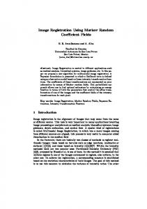
In this section, we briefly describe the architecture of the Connection Machine CM2. A more detailed description can be found in Ref. [28]. The Connection Machine is a single instruction multiple data (SIMD) parallel computer with 8 K to 64 K processors. Each processor is a l-bit serial processor, with 32 K bytes of local memory and an 8 MHz clock. The Connection Machine is

290

M. Berthod et al./Image and Vision Computing I4 (1996) 285-295 Table 2 Results on the ‘triangle’

Front End

Algorithm

VPR

image with four classes

No. of Iter

Micro-controller

. . . I

Memory

ICM Metropolis Gibbs MMD GSA DPA

NEWS Router

-

Procs

Communications

Fig. 1. CM-2 architecture.

accessed via a front-end computer which sends macroinstructions to a microcontroller. All processors are cadenced by the microcontroller to receive the same nano-instruction at a given time from it. Physically, the architecture is organised as follows (Fig. 1): l l

l

The CM2 chip contains 16 l-bit processors. A Section is the basic unit of replication. It is composed of 2 CM2 chips, the local memory of the 32 processors and the floating point unit. The interprocessor communication architecture is composed of two distinct networks: - A nearest-neighbour network, the NEWS Network (North-East-West-South), interconnects processors in groups of four. - A more complex network, called the Router Network, is used to provide general communication between any pair of processors. Each group of 16 processors is connected to the same router, and each router is connected to 12 other routers forming a 12dimensional hypercube.

For a given application, the user can dynamically define a particular geometry for the set of physical processors that has been attached. The processor resource can be virtualised (VP Ratio) when the number of data elements to be processed is greater than the number of physical processors. In such Table 1 Results on the ‘chess board’ Algorithm


VPR

2 2 2 2 2 2

8 316 322 357 20 164

Total time

Time per It.

(s)

(s)

0.078 7.13 9.38 4.09 0.20 2.82

0.009 0.023 0.029 0.011 0.010 0.017

9 202 342 292 31 34

Time per It.

(sl

(s)

0.146 7.31 14.21 7.41 0.71 1.13

0.016 0.036 0.042 0.025 0.023 0.033

Energy

49209.07 44208.56 44190.63 44198.31 45451.43 44237.36

a case, several data elements are processed on a single physical processor. Note that when the VP Ratio increases, the efficiency of the machine also increases, because the instruction is only loaded once. For the three algorithms described in this paper, we use data parallelism on a square grid (one pixel per virtual processor) and the fast local communications (NEWS). Such an architecture is well suited for computer vision as it is expressed in Ref. [29]. 6.2. Model for image classiJication Using the same notation as in section 2, we want to maximise P(L/ Y) as defined in Eq. (3). We suppose that P( ,vi/Li) is Gaussian: p(YiILi)

= gjLi

exp

(-(Y;i-J))

(15)

where pLi (1 5 Li 5 M) is the mean and gLL,is the standard deviation of class Lie It is obvious from Eq. (3) that this expression with a factor l/T corresponds to the energy potential of cliques of order 1. The second term of Eq. (3) is Markovian: P(L) = exp(-q)

= exp

-f (

Y(Ls,,Ls,)

=

= exp(-+z

c

vcL)

P$Lsi,Lsj)

{si>sjlEq

-1

if Lsi = Ls,,

+l

ifLs,#Ls,,

(17)

Table 3 Results on the ‘noise’ image with three classes

image with two classes

No. of Iter

2 2 2 2 2 2

Total time

Energy

52011.35 49447.60 49442.34 49459.60 50097.54 49458.02

Algorithm


VPR

2 2 2 2 2 8

No. of Iter

8 287 301 118 17 15

Total time

Time per It.

(s)

(s)

0.302 37.33 35.76 10.15 1.24 1.33

0.037 0.130 0.118 0.086 0.073 0.089

Energy

-5552.06 -6896.59 -6903.68 -6216.50 -6080.02 -6685.52

M. Berthod et al./Image

and Vision Computing

where /3 is a model parameter controlling the homogeneity of regions. We get the estimation of L, denoted by L, as follows: i=

arg max LEY $nP(YIL) ( argyGa;

2 (

-f

Using the above equation, it is easy to define the global energy dfglob(L) and the local energy a,(L) at site Sj of labelling L:

+lnPiL))

- f

In J%gL, + (

i=l

c

(Vi -

2_

ILL I*

’

L,

)

(19)

P”Iv5,JsJ

{S,.S,}FM

J

8,(L) = f = arg min LEY

+;

291

14 (1996) 285-295

5 (

c

In fiaL,

f

i=l

i

+ ili~O~‘2 L,

Original

DPA

(Yi - &I2 2D2 L,r

)

(20)

t

)

image

+

C

PGS,>Ls,)

{s,.s,}t-%

InGaL,

(18)

Noisy

image

Gibbs

Sampler

(SNR=

GSA Fig. 2. Results on the ‘chess board’

-5dB)

Initialization

Metropolis

MMD image with two classes.

of ICM,

DPA,

GSA

292

M. Berthod et aLlImage and Vision Computing 14 (1996) 285-295

6.3. Experimental results The goal of this experiment is to evaluate the performance of the three algorithms (DPA, GSA and MMD) proposed by the authors. We compare these algorithms with three well-known MRF based methods: ICM [3,4], a fast, deterministic relaxation scheme; Metropolis Dynamics [lo]; and Gibbs Sampler [I]. The last two are classical fully-stochastic relaxation techniques. The performances are evaluated in two respects for each algorithm: the reached global minimum of the energy function and the computer time required. We remark that in all cases, the execution is stopped when the energy change AU is less than 0.1% of the current value of 6. We display experimental results on the following images: 1. ‘chess board’ image 128 x 128 (Fig. 2)

with

2 classes,

pixel

size:

Noisy

image

ICM

Gibbs

Sampler

DPA

GSA

Original

image

(SNR.=

Fig. 3. Results on the ‘triangle’

2. ‘triangle’ image with 4 classes, pixel size: 128 x 128 (Fig. 3), 3. ‘noise’ image with 3 classes, pixel size: 256 x 256 (Fig. 4) 4. a SPOT image with 4 classes, pixel size: 256 x 256 (Fig. - 5). Tables l-4 give, for each image and for each algorithm, the Virtual Processor Ratio (VPR), the number of iterations, the computer time, and the reached minima of the energies. Note that only the relative values of the energies matter. The following parameters are used for the experimentation: l

Initialisation of the labels: Random values are assigned to the labels for the initialisation of the Gibbs, Metropolis and MMD algorithms. For the ICM, DPA and GSA techniques, the initial labels are obtained using only the Gaussian term in Eq. (18) (for ICM, this

3dB)

Initialization

Metropolis

MMD image with four classes.

of ICM,

DPA,

GSA

293


Original

image

ICM

Noisy

image

Initialization

Gibbs

Sampler

Metropolis

DPA,

GSA

MMD

GSA

DPA

of ICM,

Fig. 4. Results on the ‘noise’ image with three classes.

l

means the ‘Maximum Likelihood’ estimate of the labels). ICM is very sensitive to the initial conditions, and better results perhaps could have been obtained with another initialisation method. Nevertheless, the ICM, DPA and GSA algorithms have been initialised with the same data for the experiment. Temperature: The initial temperature for those algorithms using annealing (i.e. Gibbs Sampler,

Table 4 Results on the ‘SPOT’ image with four classes Algorithm


VPR

8 8 8 8 8 8

No. of Iter

8 323 335 125 22 15

Total time Time per It. (s)

(sl

0.381 42.31 46.73 10.94 1.85 1.78

0.048 0.131 0.139 0.087 0.084 0.119

Energy

-40647.96 -58037.59 -58237.32 -56156.53 -56191.61 -52751.71

Metropolis, MMD) is TO = 4, and the decreasing schedule is given by T,,, = 0.95 Tk. For other algorithms (i.e. ICM, DPA, GSA), T = 1. Mean and standard deviation of each class: They are computed using a supervised learning method. Their values are listed in Table 5. Choice of ,B: ,!3 controls the homogeneity of regions. The greater the value of p is, the more we emphasise the homogeneity of regions. The values of p used for different images are shown in Table 6. Table 5 Model parameters

chess board

for the four images

119.2

659.5

149.4

691.4

-

triangle noise

93.2 99.7

560.6 94.2

116.1 127.5

588.2 99.0

139.0 159.7

547.6 100.1

_

162.7 495.3 _

_

SPOT

30.3

8.2

37.4

4.6

61.3

128.1

98.2 127.1

M. Berthod et aLlImage and Vision Computing I4 (1996) 285-29s

294

Original

Initialization

image

ICM

Gibbs

DPA

GSA Fig. 5. Results

l

Sampler

P

(Y(for MMD)

chess board triangle noise SPOT

0.9 1.0 2.0 2.0

0.3 0.3 0.1 0.7

GSA

Metropolis

on the ‘SPOT’ image (four classes).

We remark that both cx and p are chosen by trial and error. As shown by Tables l-4 and Figs. 2-5, stochastic schemes are better regarding the achieved minimum, thus the classification error; deterministic algorithms are better regarding the computer time. ICM is the

Image

DPA,

MMD

Choice of a! for MMD: a regulates the speed of the algorithm of MMD as well as its degree of randomisation. The values of (Y for different images are also shown in Table 6.

Table 6 The 0 value, and the (Yvalue for MMD

of ICM,

fastest, but the reached minimum is much higher than for the other methods (as mentioned earlier, another initialisation might lead to a better result, but a more elaborate initialisation usually increases the computer time). DPA, GSA and MMD seem to be good compromises between quality and execution time. Sometimes the results obtained by these algorithms are very close to the ones of stochastic methods. On the other hand, they are much less dependent on the initialisation than ICM, as shown by the experiment results and also in the theoretical aspects. Note that, in Fig. 4, we are lucky that the maximum likelihood initialisation is very close to the true solution. But it is not generally the case. ICM improves the results in other figures, but not really in Fig. 4 because, on this particular image, the initial conditions are really good. It should be noticed that the three proposed algorithms do about the same when averaged across the different test images. It is impossible to say that one


approach is better than the others. The choice of using which one of these methods is a question of taste. Finally, we remark that the random elements in GSA and in MMD are different from each other, and also different from that in simulated annealing schemes. In GSA, candidate labels are chosen in a deterministic way. Only the acceptance of the candidate is randomised. In MMD, the choice of the new label state is done randomly, and the rule to accept a new state is deterministic. In simulated annealing, both the selection and the acceptance of candidates are randomly decided.

7. Conclusion In this paper, we have described three deterministic relaxation methods (DPA, GSA and MMD) which are suboptimal but are much faster than simulated annealing techniques. Furthermore, the proposed algorithms give good results for image classification and compare favourably with the classical relaxation methods. They represent a good trade-off for image processing problems. It should be noticed that the three algorithms have about the same performance when averaged across the different test images. Until now, we have used them in a supervised way, but an interesting problem would be to transform them into fully data-driven algorithms. This should be done using parameter estimation techniques such as Maximum Likelihood, Pseudo-Maximum Likelihood or Iterative Conditional Estimation, for instance. Finally, the three proposed methods could be adapted to multi-scale or hierarchical MRF models.

Acknowledgements

This work has been partially funded by CNES (French Space Agency). The data shown in Fig. 3 was provided by GdR TdSI (Working Group in Image and Signal Processing) of CNRS.

References 111S. Geman and D. Geman,

Stochastic relaxation, Gibbs distributions and the Bayesian restoration of images, IEEE Trans. Patt. Analysis and Mach. Intel., 6 (1984) 721-741. 121R. Azencott, Markov fields and image analysis, Proc. AFCET, Antibes, France, 1987. 131J. Besag, On the statistical analysis of dirty pictures, J. Roy. Statis. Sot. B., 68 (1986) 259-302. Random [41 F.C. Jeng and J.M. Woods, Compound Gauss-Markov Fields for image estimation, IEEE Trans. Acoust., Speech and Signal Proc., 39 (1991) 638-697. MIT Press, 151A. Blake and A. Zisserman, Visual Reconstruction, Cambridge, MA, 1987.

161A. Rangarajan

2%

and R. Chellappa, General&d graduated nonconvexity algorithm for maximum a posteriori image estimation, Proc. ICPR, June 1990, pp. 127-133. 171D. Geiger and F. Girosi, Parallel and deterministic algorithms for MRFs: surface reconstruction and integration, Proc. ECCV90, Antibes, France, 1990, pp. 89-98. using PI J. Zerubia and R. Chellappa, Mean field approximation compound Gauss-Markov random field for edge detection and image restoration, Proc. ICASSP, Albuquerque, NM, 1990. [91 P.V. Laarhoven and E. Aarts, Simulated Annealing: Theory and applications, Reidel, Dordrecht, Holland, 1987. M. Rosenbluth, A. Teller and [lOI N. Metropolis, A. Rosenbluth, E. Teller, Equation of state calculations by fast computing machines, J. Chem. Physics, 21 (1953) 1087. 1092. [Ill H. Derin, H. Elliott, R. Cristi and D. Geman, Bayes smoothing algorithms for segmentation of binary images modeled by markov random fields, IEEE Trans. Patt. Analysis and Mach. Intel., 6 (1984). WI 0. Faugeras and M. Berthod, Improving consistency and reducing ambiguity in stochastic labeling: an optimization approach, IEEE Trans. Patt. Analysis and Mach. Intel., 4 (1981) 412-423. [I31 R. Hummel and S. Zucker. On the foundations of relaxation labeling processes, IEEE Trans. Patt. Analysis and Mach. Intel., 5(3) (1983) 267-287. v41 R.H.A. Rosenfeld and S.W. Zucker, Scene labeling by relaxation operation, IEEE Trans. Systems, Man and Cybernetics, 6(6) (1984) 420-433. [151 H.I. Bozma and J.S. Duncan, Integration of vision modules: a game-theoretic approach, Proc. Int. Conf. Computer Vision and Pattern Recognition, Maui, HI, 1991. pp. 501-507. P61 H.I. Bozma and J.S. Duncan, Modular system for image analysis using a game-theoretic framework, Image & Vision Computing. lO(6) (1992) 431-443. [17] D.A. Miller and S.W. Zucker. Copositive-plus Lemke algorithm solves polymatrix games, Oper. Res. Letters, 10 (1991) 2855290. [18] D.A. Miller and S.W. Zucker, Efficient simplex-like methods for equilibria of nonsymmetric analog networks. Neural Computation, 4 (1992) 1677190. [19] T. Basar and G.J. Olsder, Dynamic Noncooperative Game Theory, Academic Press, New York, 1982. [20] M. Berthod, L’amelioration d’etiquetage: une approche pour l’utilisation du contexte en reconnaissance des formes. These d’etat, Universite de Paris VI, December 1980. [21] M. Berthod, Definition of a consistent labeling as a global extremum. Proc. ICPR6, Munich, Germany 1982, pp. 339.-341. [22] J.E. Besag, Spatial interaction and the statistical analysis of lattice systems (with discussion), J. Roy. Statis. Sot. B. 36 (1974) 192236. [23] A.bBerman and R. Plemmons, Non-negative Matrices in the Mathematical Sciences, Academic Press, New York, 1979. [24] L. Baratchart and M. Berthod, Optimization of positive generalized polynomials under If constraints. Technical report, INRIA, France, 1995. (251 S. Yu and M. Berthod, A game strategy approach to relaxation labeling, Computer Vision and Image Understanding, 61(l) (January 1995) 32-37. [26] J.F. Nash, Equilibrium points in n-person games, Proc. Nat. Acad. Sci. USA, 36 (1950) 48-49. [27] Z. Kato, Modelisation Markovienne en classification d’image mise en oeuvre d’algorithmes de relaxation. Rapport de stage de DEA, Universite de Nice, 1991. [28] W.D. Hillis. The Connection Machine, MIT Press, Cambridge, MA, 1985. [29] J. Little, G. Belloch and T. Cass, Algorithmic techniques for computer vision on a fine-grain parallel machine, IEEE Trans. Patt. Analysis and Mach. Intel. 11 (1989) 2444257.