Calculating and understanding the value of any type of match evidence when there are potential testing errors Norman Fenton1 Martin Neil2 and Anne Hsu3 25 September 2013 THIS IS A PRE-PUBLICATION DRAFT OF THE FOLLOWING CITATION Fenton, N. E., Neil, M., & Hsu, A. (2014). "Calculating and understanding the value of any type of match evidence when there are potential testing errors". Artificial Intelligence and Law, 22. 1-28 http://dx.doi.org/10.1007/s10506-013-9147-x
Abstract It is well known that Bayes’ theorem (with likelihood ratios) can be used to calculate the impact of evidence, such as a ‘match’ of some feature of a person. Typically the feature of interest is the DNA profile, but the method applies in principle to any feature of a person or object, including not just DNA, fingerprints, or footprints, but also more basic features such as skin colour, height, hair colour or even name. Notwithstanding concerns about the extensiveness of databases of such features, a serious challenge to the use of Bayes in such legal contexts is that its standard formulaic representations are not readily understandable to non-statisticians. Attempts to get round this problem usually involve representations based around some variation of an event tree. While this approach works well in explaining the most trivial instance of Bayes’ theorem (involving a single hypothesis and a single piece of evidence) it does not scale up to realistic situations. In particular, even with a single piece of match evidence, if we wish to incorporate the possibility that there are potential errors (both false positives and false negatives) introduced at any stage in the investigative process, matters become very complex. As a result we have observed expert witnesses (in different areas of speciality) routinely ignore the possibility of errors when presenting their evidence. To counter this, we produce what we believe is the first full probabilistic solution of the simple case of generic match evidence incorporating both classes of testing errors. Unfortunately, the resultant event tree solution is too complex for intuitive comprehension. And, crucially, the event tree also fails to represent the causal information that underpins the argument. In contrast, we also present a simple-toconstruct graphical Bayesian Network (BN) solution that automatically performs the calculations and may also be intuitively simpler to understand. Although there have been multiple previous applications of BNs for analysing forensic evidence – including very detailed models for the DNA matching problem, these models have not widely penetrated the expert witness community. Nor have they addressed the basic generic match problem incorporating the two types of testing error. Hence we believe our basic BN solution provides an important mechanism for convincing experts – and eventually the legal community – that it is possible to rigorously analyse and communicate the full impact of match evidence on a case, in the presence of possible errors.
Keywords: Bayes, likelihood ratio, forensic match, evidence
1
Professor and Director of Risk and Information Management Research Group (Queen Mary University of London) and CEO Agena Ltd. Email:
[email protected] 2
Professor of Computer Science and Statistics (Queen Mary University of London) and Director, Agena Ltd. Email:
[email protected] 3
1
Queen Mary University of London
1. Introduction Correct probabilistic reasoning has the potential to dramatically improve the efficiency and quality of the criminal justice system. Central to probabilistic reasoning is Bayes’ theorem: a mathematical rule prescribing the correct way for updating the probability of a hypothesis given new evidence [5][8][11][13] [26] [45][47]. The application of Bayes’ theorem to probabilities is akin to the application of addition or multiplication to numbers: probabilities are either correctly combined by this rule, or they are combined incorrectly by other means. However, much contention surrounds the use of Bayes in the courtroom, not least because its formulaic analyses are often complicated, especially to lawyers, judges and juries, who are typically untrained in statistics. Presenting even a ‘simple’ Bayesian calculation using the standard formulaic approach, such as Figure 1, is clearly not feasible in court.
V
P( H p | E , I1 , I 2 ) P( H d | E , I1 , I 2 )
P( E | H p ) P( I1 | H p ) P ( I 2 | H p ) P ( H p ) P( E | H d ) P( I1 | H d ) P( I 2 | H d ) P( H d )
Figure 1 A typical Bayesian calculation: well beyond the comprehension of lawyers and juries
Indeed, it was an attempt based on this exact example, that led to the ruling in [1] that: “The introduction of Bayes' theorem into a criminal trial plunges the jury into inappropriate and unnecessary realms of theory and complexity deflecting them from their proper task” The difficulties in understanding Bayesian reasoning were exemplified in the recent, highly profiled case of R v T [1], where the English Court of Appeal ruled that the use of formulas to calculate probabilities and reason about the value of evidence was inappropriate in areas such as footwear mark evidence where there was no ‘firm scientific base’. Although there have been many critiques of the ruling ([6][10] [40] [46] [53] [48]) it is directly impacting the way forensic experts analyse and present evidence to courts (we present actual examples of its potentially damaging impact below). One of the objectives of this paper is to explain why correct Bayesian reasoning about the impact of evidence on a case is so challenging for courts and also expert witnesses themselves. We focus on the generic case of match evidence, which we introduce in Section 2. Our notion of a ‘match’ applies to all types of evidence (not just that which comes under the standard category of forensics). A match could refer to some feature of a person ranging from DNA, fingerprints, or footprints through to more basic features such as skin colour, height, hair colour or even name. But it could also refer to non-human artefacts (and their features) related to a crime or crime scene, such as clothing and other possessions, cars, weapons, soil etc. In all cases a standard approach to evaluating the impact of a ‘match’ is to compute the likelihood ratio (the probability of finding the match if it belongs to the target divided by the probability of finding the match if it does not belong to the target); of course, this requires access to statistical data and/or expertise about the frequency of the feature in the relevant population. Notwithstanding concerns (as raised in RvT) about the rigour of such data, there are two challenges: 1. Ensuring the probability calculations are correct 2. Explaining to lay people how the results were arrived at and what they mean It turns out, as we show in Section 3, that with certain extremely simplified assumptions (notably that there is a single piece of match evidence and every aspect of the matching and testing process is ‘perfect’ so there is no possibility of matching errors), challenge 1 is sufficiently simple for any type of evidence expert to do by hand. And for challenge 2 with these assumptions it is widely assumed that the underlying Bayesian arguments can be easily
2
explained to lay people by using event trees (or some equivalent like population diagrams) annotated with frequency values for probabilities of events [29]. However, as soon as things get more complex, such as where there are multiple pieces of dependent evidence or where the profile of a single matched feature is based on multiple interdependent components (such as the loci of DNA, or the characters in a car number plate) it is impossible to do the calculations manually, let alone explain them to lay people. Although probability experts have addressed some of these complexity problems extensively in the special case of DNA match evidence (notably, by using sophisticated Bayesian network models [17][18][54]) these methods have not widely penetrated the expert witness community. Moreover, even if we ignore the complexity of dependent profile components, there is an extremely important additional complexity that generally must be considered in the simplest case: this is the need (highlighted by the likes of Koehler [36][37][38] and Thompson [55][56]) to incorporate the possibility of matching errors (false positives and false negatives) that can occur at various stages of investigation and testing and which can have a devastating impact on the value of the evidence. It turns out that, even in the simplest case, in practice expert witnesses are either not aware of the need to incorporate the possibility of errors in their analysis or they do not know how to do it. Indeed, on the basis of several dozen confidential reports from expert witnesses that we have been asked to scrutinize in the last 5 years, we believe that in practice proper analysis (i.e. accounting for possible testing errors) is not undertaken even in the simplest case. The experts tend to simply ignore the challenge, making assumptions that are unrealistic (and often demonstrably false). This results in presentation of the impact of their evidence that is often misleading and fundamentally flawed. The expert reports we have examined (primarily, but not exclusively from forensic scientists) considered different types of match evidence in murder, rape, assault and robbery cases. The match evidence includes not just DNA, but also handprints, fibre matching, footwear matching, soil and particle matching, matching specific articles of clothing, and matching cars and their number plates (based on low resolution CCTV images). Although the DNA experts in many of these cases provided explicit probability statements (such as “the probability that the trace found came from a person unrelated to X is less than one in a billion”) the other experts have invariably provided verbal quasi-probabilistic statements instead, most typically in the following format: “.. the probability/chances that Y belongs to anybody other than X is so small that it can be discounted4” “.. the probability/chances that Y comes from anything/anywhere other than Z is so small that it can be discounted” “ the evidence provides moderate/strong/very strong support for the proposition that Y belongs to /comes from X” In all cases there was some kind of database or expert judgement on which to estimate frequencies and ‘random match’ probabilities, and in most cases there appears to have been some attempt to compute the likelihood ratio. The verbal scale (ranging from “weak or limited support”, through to “extremely strong support”) is typically based on a Forensic Science Service Guide described in [43] that is a direct mapping from the likelihood ratio. For example, “moderately strong support” corresponds to a likelihood ratio of between 100 and 1000.
4
We also found lawyers who automatically assumed that evidence of fingerprint and DNA ‘matches’ were synonymous with ‘identification’ – an issue explained in [34] and [49].
3
However, in all but the DNA cases the explicit statistics and probabilities were not revealed in court – in several cases this was as a direct result of the RvT ruling. Indeed, we have seen expert reports that contained the explicit data being formally withdrawn as a result of RvT. This is one of the key negative impacts of RvT - we feel it is extremely unhelpful that experts are forced to suppress explicit probabilistic information; stating “moderately strong support” instead of a specific likelihood ratio of, say, 200 is an unnecessary loss of important expert information. However, of far greater concern is the fact that in not one report did the experts make any attempt to incorporate into their explicit (or implicit) calculations the probabilistic uncertainty of match errors. Where experts considered the possibility of match errors at all it was only in the context of cross-contamination, which in generic terms can be considered as the case where the trace being tested is not the same as the trace associated with the crime or crime scene. In all such cases the experts simply dismissed such a possibility as either “impossible” or “so small that it can be discounted”. In Section 4 we provide a generic ‘solution’ to the case of a single piece of match evidence incorporating the possibility of testing errors. Although the paper [55] considered (for DNA evidence) the case with false positives, we believe ours is the first generic solution incorporating the possibility of both false positives and false negatives. The solution in Section 4 is an event tree version. Unfortunately, even for such a constrained and simplified version of the problem this approach becomes computationally difficult and far too complex for intuitive comprehension (and might lead to a lack of trust in the transparency and accuracy of the results). We also argue that event trees do not adequately allow the unambiguous representation of the sorts of causal knowledge implicit in legal arguments linking hypotheses together with evidence. The calculations represented by, and carried out, using event trees are static versions of the kinds of adaptive, flexible calculations that can be much more easily and rapidly carried out using Bayesian Network (BN) technology. Hence, in Section 5 we present the generic BN solution. In stark contrast to event trees, the simple-to-construct BN solution not only automatically performs the calculations necessary to quantify the value of the match evidence, but may also be intuitively simpler to understand. For more complex versions of the problem BNs provide the only currently available method for doing the necessary calculations. We stress again that the use of BNs for probabilistic analysis of forensic evidence is by no means new (see, for example [8][15][16][24][26][31][32][41][50][53][54] and also [11][12][35][58] for related evidence argumentation approaches) and our solution does not represent the stateof-the-art of BN analysis for the special case of DNA (which can be found in articles such as [15][41]) but what we present is the first simple generic BN solution to this specific problem, in a way that we feel could be presented and used by practitioners. Based on previous experience of using BNs to help lawyers understand the impact of evidence [24][26], we feel that the BN solution can be used to more easily and accurately perform the necessary probabilistic analyses. However, we do not claim that such a solution is ready to be used in court. Instead, in Section 6, we recommend a process whereby legal professionals can trust the mathematical correctness of Bayesian calculations, in the same way as one would trust a calculator to carry out arithmetical calculations. Once they are assured of the mathematical certainty of the Bayesian method, legal professionals can then productively focus debate on the aspects of Bayesian calculations that are disputable and often very difficult: how evidence translates into the prior assumptions and probability values that are input into the calculation process.
2. The simplest generic evidence ‘match’ problem In order for our analysis and recommendations to be as widely applicable as possible we consider a generic framework for the notion of evidence matching. It is applicable to, just about, any current and future area of forensic science involving physical properties of human beings, what they wear, and what they own. It also applies to areas of evidence not considered
4
as forensics but where there is a valid notion of ‘match’ evidence. To give a feel for why it is much broader than just DNA it includes the following diverse examples (in each case we want to know probabilistic impact of the match evidence): 1. In fleeing a crime the person believed to have committed it stumbles leaving a shoe he was wearing at the scene. A shoe expert determines the size of the shoe to be 14. A suspect is examined and found to have feet requiring size 14 shoes. Hence, the suspect’s shoe size ‘matches’ that found at the scene5. 2. An eyewitness to a crime states that the criminal had the following identifiable features: sex (male), complexion (East Asian) height (between 200 and 210 cm) and hair colour (light-coloured). Fred is a man, Malaysian, 206.8 cm tall (to one decimal place), with blonde hair. Hence Fred ‘matches’ the person seen by the eye witness. 3. A fragment of a cheque is left at a crime scene. A cheque expert asserts that the first three numbers “3280” of the nine-digit account code are on the cheque. A suspect’s cheque account code is “328019456” and hence ‘matches’ that found at the scene. 4. A blurred CCTV image from a crime scene reveals a car number plate. A car number plate expert (aided by an image expert) determines that it is a 7 character number, in which the first character is either R or P, the third and fourth are numbers 5 and 6 respectively and the last is M or N. The suspect owns a car with number plate PC56 KRM, and hence it ‘matches’ that found at the scene. 5. A Harrods’s label grey bomber jacket with distinctive embroidered emblem of a cockerel sitting on a football is found at the crime scene. A CCTV image of a suspect captured the day before the crime shows him wearing a grey bomber jacket with an emblem resembling a bird. Hence the jacket found at the scene matches the one the suspect was known to wear. 6. Soil found on a suspect’s car the day after a crime is determined by soil experts to contain two fairly rare hydrocarbon compounds. The soil at the crime scene contains the same two hydrocarbon compounds and hence matches the soil found on the suspect’s car. 7. A recording of an emergency telephone call made by a murder victim shortly before his death includes the statement “Xavier is trying to kill me”. A man called Xavier Voss lives a mile from the victim and hence matches the name of the assumed murderer. 8. A voice expert compares the voice in the telephone call (in 7 above) with a clear recording of a speech the victim made at his daughter’s wedding and determines that the voice patters are sufficiently similar that they match. From the above examples, it may be seen that in general match evidence is characterised by the following concepts:
5
Feature and Trace: There is one or more feature (such as DNA, voice, size, code, and colour) of either a person, a person’s belongings or clothing, or an object associated with the person or crime scene that is found in the form of a trace. For a person the trace can be found in the form of actual human tissue (blood, semen, hair, skin, etc.), a type of ‘print’ (such as a fingerprint, handprint, footprint, ear print etc);
Note that even if the suspect is determined to have feet requiring size 13 or 14 shoes, we would still refer to it as a ‘match’; thus, we deliberately avoid using the term ‘consistent with’ even though forensic scientists typically use that expression rather than ‘match’ in such situations. The distinction between ‘match’ and ‘consistent with’ is actually artificial and leads to much confusion since it suggests, wrongly, that a ‘match’ is somehow unique. Even using the term ‘exact match’ to distinguish “14” from “13 or 14” is potentially misleading because again it wrongly implies uniqueness.
5
or a ‘record’ (such as an image from a CCTV, an eye witness statement, a sound recording, or even a birth certificate). Similarly, for an article of clothing or object the trace can be in the form of a physical part of the object (ranging from a single fibre or particle through to the entire item left at the scene); a type of print (such as shoe print, tyre print, etc) or a ‘record’ (such as from a CCTV, eye witness statement, or invoice).
Profile: The profile, X, of the feature is some set of identifiable markers or parameters that can be determined from the trace; for example, the profile of the cheque account code is a set of up to 9 numbers (depending on how many are visible); for any type of ‘print’ the profile could be as simple as the specific length and width or as complex as a thousand shape parameters depending on the type and quality of print; for human tissue the feature of interest would normally be DNA and the profile would normally be in the form of a number of specific DNA loci (where the number depends on the quality of the trace); but where the trace is a record the profile of a feature such as ‘height’ of a person could be as simple as a single number or range.
Source, target, and reference trace: The trace found at the scene is called the source trace, from which we determine the profile of the feature of interest In addition, we assume that there is a person (normally but not always the defendant) or object from which it is possible to get a trace, referred to as the target trace, and from which it is possible to determine the profile of the feature of interest. So, in Example 1 the cheque fragment is the source trace, and the account code is the feature of the bank account we are interested in. The target trace could be a cheque or bank statement taken from the defendant, from which we determine the profile of the account code and the target trace. Normally the profile of the source trace contains less ‘information’ than the profile of the target trace (but there are cases where the situation is reversed such as in Example 4 above where the whole item is found at the scene rather than in the possession of the defendant). For example, the profile of the ‘source’ cheque in our example has just the first four numbers of the account code whereas the profile of the ‘target’ cheque has all 9 numbers. Whichever trace contains the more information is referred to as the reference trace.
Match: The evidence E of a match is the observation that the profile of the less informative trace, be it source or target, is a subset of the profile of the reference trace.
To keep things as simple as possible we focus on the simplest possible case of match evidence where there is just a single marker/parameter that characterises the feature of interest. Example 1 is fine since the shoe ‘size’ is characterised by a single number or number range. Example 3, is also fine because as long as the numbers in a cheque account code can be considered random and independent of each other, then we can treat the entire code number as a single marker. Similarly, example 7 is fine providing the feature is restricted to ‘first name’ rather than full name. However, in contrast, in Example 4 the components of a car number plate are not all random and independent; for example, the third and fourth characters are normally digits corresponding to a particular year code (56 means the car was first registered in the second half of the year 2006). As a rule of thumb, if there is more than one marker required to characterise the feature then we need to ask the following questions:
6
Do the different markers require different tests or types of tests (which may have different levels of accuracy)?
Are there dependencies between any of the different markers (e.g. does the value of one influence the value of another)?
Do the values of different marker have different prior frequencies?
If the answer to any of these questions is ‘yes’ (as in Examples 2,4,5,6,8 above) then the correct probabilistic modelling of the match ‘as a whole’ is beyond the scope of this paper. DNA is another example where the individual markers are not genuinely independent and hence where correctly handling match probabilities requires sophisticated Bayesian network models [17][18][41]. The fact that there were dependencies between the markers (that may not have been rigorously handled) in the RvT shoeprint case was one of the problems highlighted. For simplicity, we will also ignore the potential for mixed profiles (especially relevant to DNA), which adds massive complexity to the problem (see, for example [15][31][54] for an understanding of the probabilistic complexities involved). However, the point we are making in what follows is that current approaches to analysing and presenting the impact of match evidence cannot adequately deal with even the simplest case; the fact that, in practice there are likely to be additional complexities actually strengthens our argument for ‘getting the basics right’. Moreover, in all of the above cases we can apply the reasoning we present to the separate markers (before worrying about how to handle the impact of dependencies).
3. Probabilistic analysis for simplest case of match evidence So, with the simplistic assumptions stated in Section 2, we wish to know what the evidence of a claimed match between the source and target trace tells us about the hypothesis H: “The source trace belongs to the defendant”. (We use ‘the defendant’ here as a simplification because we could equally replace it with ‘the victim’, or any other relevant person, item or object associated with the crime or crime scene). Thus, in example 1 above this means we want to know what the matching shoe size evidence tells us about the hypothesis that the shoe found at the scene actually belongs to Fred. This example is deliberately chosen not just for simplicity but because it highlights a fundamental flaw in the RvT ruling, which assumed there is a clear distinction between forensics with a ‘firm statistical’ base (of which DNA was cited as an example) and that for which there is not (of which footwear was cited). In reality getting accurate statistics on shoe size frequency is more realistic than getting accurate statistics on DNA profile frequency. In probabilistic terms the question we are asking is: How does the probability of H change after we observe the evidence E. For example, if the shoe size is extremely rare in the population then the impact of the evidence on H is far greater than if the shoe size is one of the most common in the population. Formally, the prior probability of H (our belief about H before seeing the evidence) is written P(H) and the posterior probability of H (our belief about H after seeing the evidence) is written P(H | E). In practice, if we assume that the profile testing is always perfectly accurate and that the entire investigation process is carried out without errors or malicious intent (meaning no possibility of the source or target traces being mixed up with any other traces at any stage), then it turns out that all we actually need in principle to determine the impact of E on H are the following two probabilities (although note that these may be extremely difficult to obtain in practice): 1. The probability of E given H (the ‘Prosecution likelihood’) written P(E | H): This is the probability that we would find the defendant’s trace profile matching the source profile if the source trace belongs to the defendant. Example: if we assume we can get a trace from the defendant that is at least as informative as the one left at the scene, and that the nature of the trace is such that it does not change much over time (e.g. DNA, shoe size, complexion and height but not
7
hair length or colour), then since we are also assuming perfect testing it is reasonable to assume that the prosecution likelihood is equal to one in this case. 2. The probability of E given not H (the ‘Defence likelihood’) written P(E | not H): This is the probability that we would find the defendant’s trace profile matching the source profile if the source trace does not belong to the defendant. Example: Suppose the trace is a shoeprint and that the matching profile is simply the size – say 14 – of the shoeprint, then a reasonable estimate of P(E | not H) would be the proportion of people who wear size 14 shoes. Although not strictly correct (see, e.g. [7]) the defence likelihood is also sometimes referred to as the random match probability or the probability of an innocent match6. Intuitively, the smaller the defence likelihood is relative to the prosecution likelihood, the greater the ‘probative value’ of the evidence in favour of the prosecution. Hence, a commonly used measure of the impact of evidence is the likelihood ratio: the prosecution likelihood divided by the defence likelihood [20]. Despite the reservations expressed explicitly about this measure in the RvT Ruling [2], it is has become a fairly standard means by which forensic scientists evaluate the impact of their evidence [5][6][20][25][40][43]. There are, however, severe limitations about exactly when the measure can be applied – as explained in depth in [27] and also [7][13][19] [30][31][39][42][50][57]. Notwithstanding these concerns about the likelihood ratio, a major reason for its popularity is that it supposedly enables forensic scientists to focus on their area of expertise without having to make any assumptions about P(H), the prior probability of H. However, as explained in several of the previously referenced critiques, there is a fundamental problem with this assumption. The (only) formal explanation for the probative value of the likelihood ratio relies on Bayes’ theorem. Specifically, (the ‘odds7 version of) Bayes’ theorem is the following formula: Posterior odds of H = Likelihood ratio × Prior odds of H It is only this formula that enables us to conclude formally that:
if the LR is greater than 1 then the larger its value the more strongly the evidence E supports the prosecution hypothesis H (because the posterior odds of H will be that much greater than the prior odds);
conversely if the LR is less than 1 then the smaller its value the more strongly the evidence E supports the defence hypothesis not H.
if the LR = 1 then the evidence E has no probative value on H because the posterior odds remain unchanged8.
6
Although the likelihoods P(E|H) and P(E| not H) are independent of the value of the prior P(H) they must take account of the same background knowledge that is implicit in the prior. For example, suppose that the prior P(H) = 0.5 is based on the background knowledge that the defendant was one of only two men known to be at the scene of the crime and both men were a similar large size. Then if E is a matching shoe size 12, P(E| not H) is certainly not the random match probability. In fact, in this case P(E | not H), like P(E | H) will be close to 1. 7
The odds of any hypothesis H (in this case the prosecution hypothesis) is simply the ratio of the probability of H over the probability of the negation of H (i.e. the defence hypothesis in this case). So the prior odds is just P(H) divided by P(not H) and the posterior odds of H is just P(H | E) divided by (P(not H | E). Odds can easily be transformed into probabilities: specifically, if the odd are x to y for hypothesis H over not H then the probability of H is x/(x + y) and the probability of not H is y/(x + y). So odds of 100 to 1 in favour of H means the probability of H is 100/101 and the probability of not H is 1/101. Also note (we will assume this later) that if the prior odds are ‘evens’ i.e. 50:50 then the posterior odds will be the same as the likelihood ratio. 8
It is important to note that, as explained in [27], these crucial properties of the LR apply only when the defence hypothesis is the negation of the prosecution hypothesis H. Forensic scientists sometimes consider defence hypotheses that are not the negation of H. In such circumstances the LR is somewhat meaningless as it tells us
8
But now we have a ‘circle to square’: the LR is popular precisely because it can be calculated without having to consider any prior probability for H [43]; but the only way to understand both why the LR is a measure of the probative value of evidence, and what the LR means in terms of impact of the evidence, is to explicitly consider P(H) the prior probability of H [39] [57] (there is also the need to consider the background knowledge involved in the prior of H as explained in footnote 4). Suppose, for example, that only one in a thousand adults have size 14 shoes; then with the above assumptions a match implies the LR of this evidence is 1000. That means the evidence E is 1000 times more likely to be observed if the prosecution hypothesis H is true than if the defence hypothesis not H is true. That sounds important but whether or not it is sufficient to convince you of which hypothesis is true depends entirely on the prior P(H). If P(H) is, say 0.5 (so the prior odds are evens 1:1), then a LR of 1000 results in posterior odds of 1000 to 1 in favour of H. That may be sufficient to convince a jury that H is true. But if P(H) is very low - say 10,000 to 1 against, then the same LR of 1000 results in posterior odds of 10 to 1 against H. That would certainly be insufficient to convince a jury that H is true. So, for anybody to really understand and accept what we mean by the impact of match evidence we have to provide an understanding of why Bayes' theorem works and this also involves considering the prior probability of H. This brings us on to a central issue of how best to explain that Bayes’ theorem is correct in the above context. A standard way to convince lay people that Bayes is correct is to put the above simple match scenario into what is commonly referred to as the ‘Island’ scenario [8]: A crime has been committed on an island. All residents are equally likely suspects. A trace from the crime scene is found - with profile X and this matches the profile of Fred. It has been determined that the random match probability is 1/100, i.e. 1 in 100 people have the trace profile type X. So, with the assumptions above P(E | not H) = 1/100 where E is the match evidence and H is the prosecution hypothesis that Fred is the source of the trace. If we assume that P(E | H) = 1 (i.e. that we would certainly find Fred's profile to be X if he was the source) then what does the evidence tell us. Specifically how does it change our belief in H? Clearly the answer to the question posed in the Island scenario depends on how many people are on the island. Suppose there are 1000 people other than Fred. This means the prior odds are 1000 to 1 against H (i.e. P(H)= 1/1001). Since the profile X occurs in about 1 in every 100 people, this means we expect about 10 of the other 1000 people to have the type X. So, once we observe the evidence (Fred has profile type X) we can rule out all other people, except those 10, as having possibly left the trace. Thus, after observing the evidence the defendant and 10 others remain as possibilities. It follows that the posterior odds of H are now 10 to 1 against. So, although the odds still favour the defence hypothesis the odds have swung by a factor of 100 (the likelihood ratio) towards the prosecution hypothesis that he is guilty. This demonstrates that Bayes’ theorem does indeed provide the correct ‘intuitive’ result. The island scenario is simple enough that it can be depicted using an event tree representation as shown in Figure 2, annotated with frequencies of events. This method has been claimed to help intuitive understanding and is considered by many as the best way to represent and communicate the variables, their states and the associated probabilities [29].
nothing about the probative value of the evidence. Moreover, [27] also showed that even when H and not H are used, the LR may tell us nothing about the probative value of E on some other hypothesis relevant to a case. In particular, this means that evidence E with an LR of one may still be probative elsewhere.
9
Figure 2: Bayesian calculation explained visually using an event tree annotated with frequencies (people who have Type X are shown in black squares) While such an event tree confirms Bayes’ theorem as ‘correct’, even for such a simple scenario there is a limitation when the random match probability is relatively low compared to the number of people on the island. For example, if there were just 10 other people on the island instead of 1000, then the event tree would have to show numbers that are a little unusual; the expected number of people who match is a fraction (one tenth) of a person. From a mathematical perspective this is not a problem: the prior odds are 10 to 1 against the prosecution hypothesis. After the evidence there is just 1/10 of another person other than the defendant, and the odds have now swung to 10 to 1 in favour of the prosecution. However, the concept of 1/10 of a person may be challenging to grasp intuitively (as indeed the original 1/100 random match probability may be). One possible method for gaining acceptance from lay people for very low match probabilities is to use hypothetical examples that do not involve fractions, and then explain that exactly the same method works no matter what the actual match probabilities are. Another possible method is to use a description such as: “Imagine 10 identical cases with the same evidence. 1/10 of a person means that out of these 10 identical cases, there will be one innocent match.” However, the example shows that, even for the most bare-bones simple case of match evidence, the standard intuitive explanations present challenges in being clearly understandable to lay people. Because many types of forensic evidence (such as from good DNA samples [21][28][43]) produce very low match probabilities, it is inevitable that we have to consider ‘fractions’ of people if we adopt this approach. Before considering what happens when we introduce the potential for testing errors, we conclude this section by presenting the generic formal event tree representation [9] for the problem specified above. Specifically, we use probabilities rather than frequencies and we break up the evidence E into two component parts. Thus
10
(Prosecution) Hypothesis H: “The defendant is the source”. Same as before, and the defence hypothesis is simply “not H”. But now we assume the prior probability P(H) is equal to s. This means that P(not H) = 1-s.
Evidence E1: The source profile type has been tested to be type X.
Evidence E2: Defendant’s profile matches the source profile (i.e. both have type X).
Figure 3: Formalized event tree determining the possible scenarios and likelihoods in simple case with no testing errors (s is the prior probability that defendant is source; m is the proportion of people who have Type X. The bold branch is that consistent with the prosecution hypothesis and the dotted branch is that consistent with the defence hypothesis)
Figure 3 shows the event tree corresponding to the Island scenario annotated with the event probabilities (conditional, but dependent on the preceding events) and branch probabilities (joint, i.e. a set of sequential events together). Thus:
The prior probabilities (probabilities of the prosecution and defence hypotheses before the evidence) are represented by the two branches in the first (left-most) fork in the tree stemming from H, which we also call ‘prior branches’. Thus, the probability when H is true is s and the probability when H is false is 1 - s.
The influences of the additional evidence are represented by the extension of the tree beyond the two ‘prior branches’. In particular, in light of the evidence, the possible scenarios under the prosecution hypothesis are shown as branches that extend from the prior branch where H = True. Similarly, the possible scenarios under the defence hypothesis are shown as branches that extend from the prior branch where H = False. Thus, in an event tree, the ‘likelihood branches’ are the remaining segments of branch which extend out from the prior branches (and do not include the prior branches). Here we assume m is the proportion of people in the population who have type X.
The Prosecution likelihood is represented by the single branch that extends out from the prior branch that assumes that H is true in Figure 3 (H = True, E1 = True, E2 = True). So, the prosecution likelihood is equal to m.
The Defence likelihood is represented by the single branch extending out from the prior branch that assumes that H is false in Figure 3 (H = False, E1 = True, E2 = True). So, the defence likelihood is equal to m2.
The likelihood ratio, which is the ratio of the prosecution likelihood over the defence likelihood, is m/m2 = 1/m.
We can read the posterior odds from the event tree diagram by summing the probabilities of all full branches where H is true and divide this by the sum of the probabilities of all full
11
branches where H is false. Note, here we refer to the probabilities of the “full branch”, which is composed of both the “prior branches” and the “likelihood branches” combined9. For the most simplistic case shown in Figure 3, which assumes no errors, the prosecution and defence hypotheses are each represented by a single full branch each, whose probabilities are shown on the right hand side of the figure. Thus the posterior odds in Figure 3 is equal to sm/[(1 - s)m2] If the values are s = 1/1000 and m = 1/100 we get posterior odds of 1/10 as above.
4. The scaling problem: extending event trees to make use of match testing error variables Whilst event trees have proven popular for representing Bayesian arguments in a number of domains (such as in safety critical applications where the likely consequences of hazards need to be assessed) their limitations are well understood [3][22]. In particular:
The causal sequence of events represented by an event tree is not sufficiently explicit to remove ambiguity.
Conditional independences between variables are implicit. Some events are considered in sequence even when preceding events have no relevance to the antecedent event in question.
A completely arbitrary sequence for the declared events is imposed. So in Figure 3 we could have declared the variables in order {H, E1, E2} or indeed {H, E2, E1}. Which order should we choose? Does it matter? In some contexts the dependency order might meaningfully reflect some causal connection between events and therefore a different order may unwittingly lead to errors by suggesting causal dependence between events where it does not exist or by separating variables in the event tree where they are in fact causally connected. Similarly, the fact there may be more than one causal agent affecting a variable is actually impossible to represent in the event tree in any satisfactory way.
A single consequential event may have one or more causes and vice versa. This is not easily represented in a tree structure, thus prohibiting the representation of whole classes of evidential relationships.
The numerical calculations carried out using event trees are static and do not change in response to evidence. Given this they are not suitable for ‘what-if’ analysis nor can they be easily amended to take account of different facts that might be presented as evidence at different times.
In addition to all of the above problems, it turns out that using an event tree simply to perform the required Bayesian calculations becomes intractable for all but the most trivial problems, even though, in principle, the analyst only has to compute the probabilities of each of the branches in the tree.
9
We use the term ‘full branch’ instead of ‘posterior branch’ because the term ‘posterior probability’ technically applies to the conditional probabilities P(H | e) and P(¬H | e), where H is the prosecution hypothesis, ¬H is the defence hypothesis, and e is the evidence. In contrast, the probability of the ‘full branches’ are actually the respective joint probabilities P(H, e) and P(¬H, e). Because P(H | e) = P(H ,e)P(e ) , the posterior odds can be equivalently written as the ratio of the posterior probabilities or the ratio of the joint probabilities. That is:
P( H | e) P( H | e) P(e) P( H , e) P(H | e) P(H | e) P(e) P(H , e)
12
It is this issue of 'scale' that we now focus on. It turns out that even the simplest case of match evidence quickly becomes too large and too difficult to understand using event trees. Here, we assume as in Section 3 that a ‘simple’ case is one in which there is only one piece of match evidence and the variables in the analysis take on simple binary, point values (in reality the problem is much more complex, involving numeric rather than binary variables and potentially multiple, related pieces of evidence etc.). We show that even with these very simplified assumptions, the introduction of basic additional features quickly makes the event tree diagram and the calculations too complicated for simple representation and communication. The basic additional features we wish to add to the simple problem are the possibilities of testing errors. Specifically we wish to consider the possibility of false positive and false negative results on the matching. There are two scenarios by which a trace might be tested as having profile X: 1. The trace has profile X and the test correctly determines it has profile X (true positive) 2. The trace does not have profile X but the test determines it has profile X (false positive) The probability of the first scenario is determined by the probability v of a false negative (i.e. a profile of type X is determined by the test to be not X) since the probability of the true positive here is 1-v. The probability of the second scenario is the probability of a false negative u. There are many reasons why the values u and v may be non-zero (as explained, for example, for the special case of DNA in [36][56]). Generally this includes inherent inaccuracies in the testing method depending on the quality of test equipment and/or experience of testing personnel; traces may get mixed up or contaminated accidently or maliciously, etc. In reality each stage where there is a potential error would have its own distinct error probability, but for simplicity we are using the ‘global’ error probabilities in what follows. As discussed in Section 1 in practice many experts assume (wrongly) that the probabilities u and v are zero (and hence that the respective probabilities of true positive and true negative are one). The authors in [55] noted that, for DNA testing, although false positive probabilities were sometimes considered they were not dealt with in the same level of rigour as the match probabilities. They asked pointedly: “Why are the two possible sources of error in DNA testing treated so differently? In particular, why is it considered essential to have valid, scientifically accepted estimates of the random match probability but not essential to have valid, scientifically accepted estimates of the false positive probability?” The authors in [55] provide a strong argument on why it is just as critical to include the false positive probability as the random match probability. However, even in this argument, the case for the false negative probability was overlooked; In fact, although several authors have tried it, we are not aware of the problem being presented correctly in any way other than by the full Bayes’ theorem formulaic approach and, even then, the presentations have not included the possibility of false negatives. The net effect is that, unless people are prepared to understand the formulas they will not be able to see that the theory agrees with personal intuitions. When we allow for the possibility of testing errors, the following relevant information must be considered:
13
Prosecution hypothesis (H1): “The defendant is the source”. This is unchanged from Section 2, although as there is now more than one hypothesis (see below) we use H1 rather than H. As before the defence hypothesis is simply the negation not H1.
Evidence E1: “The source profile is tested to be of type X” (note: we can no longer assume the source profile actually is type X)
Evidence E2: ”The defendant profile is tested to be of type X (note: we can no longer assume the defendant profile actually is type X)
Because of the probability of false positives we cannot assume from the above evidence that either the source or the defendant profile is type X. Instead these assertions are also unknown hypotheses:
Source type hypothesis (H2): “The source profile really is type X” (true or false)
Defendant type hypothesis (H3): “The defendant profile really is type X” (true or false)
What we have, therefore, is a problem involving five ‘variables’ H1, H2, H3, E1, E2 which can all be true or false. But this means there are 32 different scenarios representing the different possible true/false combinations (although some are not observed, such as the evidence being false, and some are logically ‘impossible’, such as the defendant is the source and the source is type X while the defendant is not type X). We can show this in the event tree diagram shown in Figure 4. Even when we ignore the impossible branches and all the scenarios in which the evidence E1 and E2 is false, we are left with six scenarios that need to be incorporated in the calculations for prosecution and defence likelihoods.
14
Figure 4 Event tree in simple case with testing errors. Here s is the prior probability that defendant is source; m is the random match probability for Type X; u is the false positive probability for X and v is the false negative probability for X (so 1- v is the true positive probability that we are interested in). The bold branch is that consistent with the prosecution hypothesis and the dotted branch is that consistent with the defence hypothesis. Cases of E1 and E2 false are not considered.
Scenarios for the prosecution likelihood include all scenarios that stem from the branch H1 = true:
Scenario 1 (this is the ‘normal’ prosecution scenario) in which H1, H2, H3, E1 and E2 are all true. This scenario has probability m(1v)2
Scenario 2 (this is an often ignored prosecution scenario) in which H1 is true (the defendant is the source) but the defendant is not actually Type X. Both the test of the defendant and source, incorrectly results in a Type X classification. This scenario has probability (1m)u 2.
Scenarios for the defence likelihood include all branches that stem from the branch H1 = False:
15
Scenario 3 (this is the ‘normal’ defence scenario) in which the tests are correct but the match is coincidental. This scenario has probability m2 (1v)2.
Scenario 4 this is the defence scenario in which the defendant is incorrectly tested to be type X. This scenario has probability m(1-m) (1v) u.
Scenario 5 this is the defence scenario in which the source is incorrectly tested as Type X. This scenario has probability (1-m) mu(1v).
Scenario 6 this is an often ignored defence scenario in which both the source and defendant are wrongly tested to be Type X. This scenario has probability (1m) 2 u2.
The prosecution likelihood is the sum of the probabilities for all scenarios that stem from the branch for the prosecution hypothesis, H1 = True: scenarios 1 and 2. The defence likelihood is the sum of the probabilities for all scenarios that stem from the branch for the defence hypothesis, H1 = False: scenarios 3, 4, 5, and 6. As in the simple tree of Section 3 (Figure 3) the posterior odds can be read from the event tree as the sum of the probabilities of all full branches where H = True divided by the summed probability of all full branches where H = False. These probabilities are shown on the right hand side of Figure 4. However, in contrast to Figure 3, there are now six full branches to consider as compared to two. Thus, the analysis is no longer sufficiently ‘simple and intuitive’ to ensure that people can check they ‘agree with personal intuition’. Resorting to explanations using Bayes’ theorem and mathematical formulas, of course, only makes things much worse. Let us just recap briefly what is going on here: we have what appears to be a very simple problem: there is a claimed match, for which we know a) the random match probability, and the b) the probabilities of a false positive and false negative. All we want to know is the likelihood ratio for the claimed match – something which any forensic scientist is supposed to be able to do routinely given that the necessary statistical information is available (ignoring all issues of whether the data is correct or not). Yet, we have shown that the required calculations for such an apparently simple computation are remarkably difficult – and that most forensic scientists (even those highly trained in statistics and probability) would not attempt to do it. The obvious temptation for experts is therefore to ignore the error probabilities, which as we already remarked, is precisely what we have observed in practice. Of just as great concern is that, even once the event tree is constructed correctly, people may fail to understand it. Indeed, recent work [51] has shown that, even for the simple matchproblem without errors, event tree representations performed significantly worse than textual descriptions in inducing correct responses to evidence interpretation from respondents. Furthermore, when errors were introduced into the problem as above, participants who saw the resulting complex event tree trusted the correct probabilistic answer less than other participants who only read word descriptions. Finally, participants who saw both simple and complex event trees felt they understood the problem significantly less than participants who saw words only. And none of the participants in any of the conditions, words or trees, felt that they trusted the calculations. In addition to these empirical concerns about the effectiveness of event trees, there are other practical and theoretical concerns. With regard to the causal interpretation of this larger event tree the difficulties inherent in getting the variable order correct are more pronounced than before. Here the variable declaration order is {H1, H2, H3, E1, E2}. However, there is a strong argument for more closely aligning the variables {H2, E1} and {H3, E2} since they are intimately causally connected; for example, H3 is the cause of E2, which is itself a measure of the true unknown state of H3. Similarly, H3 and H1 are clear causes of H2 yet rather than state the probability of H2 given H3 and H1, i.e. P(H2 | H3, H1), we are forced to consider the unnatural variable order in the event tree. The example also shows that, even for experienced Bayesians, it can be difficult to model the problem in a sensible way and difficult to perform the calculations (as we mentioned earlier,
16
we have not previously seen a full solution of this problem in the literature, taking into account both types of error probabilities). And this example still has many simplifications: it assumes that all three probabilities random match, false positive, and false negative are all ‘point’ values, whereas in practice they would be uncertain distributions [8]; it assumes that all variables have just two possible values (true and false); it assumes that there is just one trace; and it assumes the only evidence is the single component match evidence. When we include further aspects of reality that are present in most cases (for example: the possibility that wrong samples were collected or analysed at different stages of the investigation; the possibility of mixture profiles; the need to incorporate other hypotheses and related pieces of evidence as well as dependencies between multiple profile components) it becomes impossible to perform the correct Bayesian calculations manually (with or without formulas) – let alone explain them to a lay person.
5. The Bayesian network solution The example analyses in Section 4 show that it is unrealistic to expect most Bayesian calculations to be presentable in an intuitively comprehensible manner using event trees. As a solution to this problem, we advocate, as others have also done [26] [54], that intuitions for Bayesian calculations may be established using such simple cases as the Island problem shown in Section 2, and these intuitions are then used to establish trust for more complex cases. For more complex cases, as most actual cases are likely to be, we need a method that allows expert witnesses and legal professionals to readily discuss the aspects of the analyses that are subject to debate: the prior assumptions, the causal relationships connecting hypotheses to evidence and probabilities that are fed into the Bayesian calculations. It is now widely accepted [54] that Bayesian networks (BNs) (see [22] for a non-technical introduction and overview) are the most suitable method for handling these types of complexity in probabilistic reasoning10. A BN performs calculations based on local dependencies among the variables that are present in a scenario. These variables include observations (e.g., evidence such as the defendant and source are tested to have profiles of type X) and hypotheses (e.g., the target was the source, the defendant and source are actually type X) related to the case. By exploiting these local dependences, a BN is typically compact and efficient. It avoids the problem present in equation-based calculations and the event tree-diagram approach depicted above which required consideration of all possible combinations of variable values and explicitly listing all possible scenarios (statisticians express this formally by saying that ‘it is not necessary to consider the full joint probability distribution’). Instead, a BN only requires consideration of how individual variables relevant to the scenario are dependent on each other, causally, and the local values these individual variables can take.
10
In fact, a Bayesian network is the most tractable way of calculating complex statistical problems for which brute-force equation-based calculations become unwieldy and even intractable. Note, the results of a Bayesian network will be mathematically equivalent to the formal manual derivations for discrete variables.
17
Figure 5: Bayesian network solution equivalent to Figure 4. Each node has states true or false
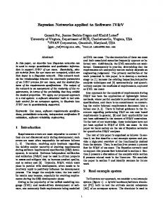
Visually, a BN can be represented as a set nodes connected by directed links (hence, it is also known as a graphical model). Figure 5 shows the graphical part of the BN solution to the problem described in Section 4 (match evidence with testing errors). The nodes correspond to the variables (which, before evidence is presented are all uncertain) and the links show the local dependency relationships between these variables. In particular, directed arrows are drawn between variables that have a direct impact on another variable. For example, whether ‘Defendant is type X’ directly impacts the chances that ‘Defendant tested as type X’. These local dependencies mean that we only need to specify how the values of a given variable depends on the values of the other variables it is linked from, i.e. other variables that have arrows pointing to the given variable (also known as ‘parent variables’). For example, in Figure 5, the graphical representation shows that the variable ‘Defendant tested as type X’ has one parent variable: ‘Defendant is type X’. This means that when setting up the BN, we only need to determine how the variable ‘Defendant is type X’ affects the variable ‘Defendant tested as type X’. In practice, determination of this local dependency means completing a table of conditional probabilities such as that shown in Table 1. Table 1 Probability table for node “defendant tested as Type X” (u is the false positive probability and v the false negative probability)
Defendant is type X:
False
True
Defendant tested as type X (False)
1-u
v
Defendant tested as type X (True)
u
1-v
The conditional probability tables for the nodes “source is type X” and “source tested as type X” are shown respectively in Tables 2 and 3. Table 2 Probability table for node “source is Type X” (u is the false positive probability, v the false negative probability, and m is the random match probability)
Defendant is type X: Defendant is the source:
18
False
True
False
True
False
True
Source is type X (False)
m
m
1-u
v
Source is type X (True)
1-m
1-m
u
1-v
Table 3 Probability table for node “source tested as type X” (u is the false positive probability and v the false negative probability)
Source is type X:
False
True
Source tested as type X (False)
1-u
v
Source tested as type X (True)
u
1-v
The probabilities for the nodes without parents (“defendant is type X” and “defendant is the source”) are simply the prior probabilities. Thus, we do not have to simultaneously consider the effects of whether ‘Defendant was the source’ or whether ‘Source is type X’. Instead the ‘distant’ dependencies between globally linked variables will be automatically calculated by the BN based on the locally linked one already specified. Formally then the relationships in the BN are structured as a graph and so allow a much richer representation of cause and effect. Mathematically Figure 4 is represented by: P(H1, H2, H3, E1, E2) = P(H3 | H1, H2)×P(E1 | H2)×P(E2 | H3)×P(H1)×P(H2) So here we can model multiple parent causes of a single effect, e.g. P(H3 | H1, H2) and then separately consider test evidence P(E2 | H3), P(E1 | H2), and the priors P(H1), P(H2). This modular structure in the BN has the benefit of supporting the elicitation and calculation of probabilities, locally, without grappling with the model as a whole. In fact this is one of the major benefits of a BN – the algorithms used to compute the answers are tractable [22] because of this modularity and the modular structure supports more efficient elicitation of model structure which is then easier to understand and much more natural for experts to consider and justify [23]. This representation is conceptually simpler than the event tree in Figure 4 because the BN represents H1, H2, H3, E1, and E2 as single nodes which can take on one of two values: true or false. Thus, all the possible scenarios shown as different branches of the event tree in Figure 4 are now represented by all the possible combinations of node states in a BN. This visual representation of a BN is readily drawn using software packages that perform BN calculations (e.g [3], which is used here). Once the relationships between nodes are defined and the probability tables are entered, we can then enter evidence as observations. The BN software automatically computes and displays the results showing how different hypotheses probabilities have been updated in response to this new evidence. The speed of this calculation allows us to readily compare how hypotheses probabilities change under varying assumptions about the evidence. This means we have the ability to dynamically test different scenarios that are impossible or difficult to do with an event tree. For example, in Figure 6 we show the results where we compare the cases: a) where we assume perfect testing accuracy, i.e. u and v are both set to zero. This is the case of no testing errors described in Section 2. b) where we assume that u (false positive) is 0.1 and v (false negative) is 0.01. This is the case of Section 3. Although in both cases we assume the same match probability m=1/100 and the same prior (50:50)11 for the prosecution hypothesis the difference is quite dramatic:
11
Recall that, by assuming a 50:50 prior, we know that the posterior odds are equal to the likelihood ratio.
19
in a) (no testing errors) the posterior odds12 are 100 to 1 in favour of the prosecution hypothesis; whereas in b) (small probability of testing errors) the posterior odds13 are only 65 to 35 (i.e. about 2 to 1) in favour of the prosecution hypothesis.
a) Impact of evidence when error probabilities are assumed to be zero
b) Impact of evidence when false positive rate is 0.1 and false negative is 0.01
Figure 6: Comparing the different impact of the evidence when we assume different error rates (in both cases the match probability is 1/100 and the prior probability for “defendant is source” is 0.5)
Not only does the BN remove the need for performing the difficult Bayesian calculations manually, but we believe that its graphical representation may be easier for a lay person to understand. The BN is also scalable with respect to incorporating the additional complexities that would be present in most realistic cases as, for example, the models in [18] demonstrate. Furthermore, complex causal assumptions linking hypotheses and evidence are more easily represented in a BN than in an event tree. We can represent common causes of single effects and multiple effects that follow from a single cause in the BN. This former case is especially important when we wish to explain away competing hypotheses that might give rise to the same consequential evidence (such as ‘Source is type X’ which is caused by ‘Defendant is type X’ and ‘Defendant is source’). Similarly, in the latter case we can represent multiple pieces of evidence each of which purport to accurately measure or indicate the same underlying causal hypothesis (in our example the cause might be ‘Defendant is type X’ and the evidential effects are ‘Defendant tested as type X’ and ‘Source is type X’). For all its intuitive benefits, we are not, however, suggesting that the BN model is what should be presented in court. Instead, we recommend that it could be used for pre-trial analysis of the evidence by forensic experts and lawyers, preferably using different scenarios for the different ranges of match probabilities and error probabilities. This is exactly the strategy that was employed successfully in a number of recent cases [24][26]; in these cases BNs were used to explain to experts and lawyers the correct probabilistic impact of evidence
12
The likelihood ratio is 100, meaning equivalently the probability the prosecution hypothesis is true is 100/101 = 99.01%) 13
The likelihood ratio is 65/35, meaning equivalently the probability the prosecution hypothesis is true is 65%).
20
that could not have been computed manually. Trust in the results was gained by first demonstrating that BN software provided the correct results in simple island-type examples. While we have provided an explicit (and immediately usable) BN solution for the generic match problem that we feel is very widely applicable, we do not underestimate the immense challenges involved in using either this same model, or other BNs when the match evidence has to take account of the further complexities we have discussed above. Even if the evidence satisfies the simple assumptions used in our model, there will generally be much disagreement about the prior probabilities required and, if they depend mainly on expert judgement rather than data, will be subject to the same inevitable legal criticism that was present in the R v T ruling. In some cases (as in [24]) it may be possible to reach the same basic conclusion by trying the fullest possible range of alternative prior probabilities, but this will not always work and may not even be feasible. In the more complex cases there will generally be no unique obvious model structure; although there has been recent work (using common patterns and idioms) to standardise the structure of BN models for legal arguments [23][32] even BN experts may disagree on the most suitable structure. However, if the model structure cannot be agreed between relevant experts and lawyers, then they should at least be able to agree about what alternatives are possible. Then, it may be feasible to consider the results not just with different prior probabilities but also with different models. All that should be presented in court are clear statements of the prior assumptions being used (notably the match probabilities, and error probabilities) and the results of the calculations under the different assumptions. We argue that it is much easier to build and run a BN model with the relevant information than it is to either construct an event tree as before or to produce the necessary formulas.
6. Conclusions and recommendations The R v T [2] ruling raised a number of fundamental concerns about the use and presentation of Bayesian arguments and likelihood ratios to show the probative value of forensic match evidence. This paper has demonstrated that presenting such evidence correctly, and in a way understandable to lay people, is extremely challenging even with the most simplistic assumptions. We have focused on the special difficulty of analysing and presenting match evidence when there is the possibility of different types of match testing errors. Because of the difficulties that this introduces, experts typically ignore it in their analyses, and hence often present their evidence in a way that is either wrong or highly misleading. We have introduced a completely generic framework for ‘match evidence’ that applies to all types of matching problems, well beyond currently accepted forensic practice. We have also presented what we believe is the first full probabilistic solution of the simple case of generic match evidence incorporating both false positive and false negative testing errors. Because event trees have been considered the most promising method for presenting Bayesian arguments to lay people, our first solution used this method of representation. Unfortunately, the necessary event tree solution is far too complex for intuitive comprehension, even in simple cases. The event tree also fails to represent or communicate the causal context that underpin legal arguments, they do not support easy calculation of the probabilities under varied and dynamic scenarios and lastly they divert attention away from the assumptions needed to ensure numerical calculations make sense and can be trusted. Because of the unsuitability of the event tree approach (and its inherent lack of scalability), we also presented a simple-to-construct graphical Bayesian Network (BN) solution that automatically performs the calculations and may also be intuitively simpler to understand. Although there have been multiple previous applications of BNs for analysing forensic evidence – including very detailed models for the DNA matching problem, these models have not widely penetrated the expert witness community – they are not accessible to forensic scientists or lawyers. Nor have they addressed the basic generic match problem incorporating the two types of testing errors. Hence we believe our basic BN solution provides an important
21
mechanism for convincing experts – and eventually the legal community – that it is possible to rigorously analyse and communicate the full impact of match evidence. It is unrealistic to expect lay people to understand complete Bayesian analyses. We believe that continued attempts to explain such arguments in legal reasoning by using first principle calculations and formulas, or event trees, will result in a doomed future for Bayes in the law. Instead, we argue that simple examples may only serve to instil confidence in the mathematical validity of Bayesian arguments. For more complex (realistic) cases, focus must be directed towards the aspects of the analyses that are subject to debate: the prior assumptions and probabilities that are fed into the calculations. In other words, the challenge over the next few years is to ensure that lawyers and experts understand the difference between: a. the genuinely disputable assumptions that go into a probabilistic argument; and b. the Bayesian calculations required to compute the conclusions based on the different disputed assumptions. Proper probabilistic approaches are commonly accepted in other areas of critical risk decision making, such as medicine and safety. In contrast, there have been significant challenges to the acceptance of probabilistic analyses in the legal domain. Future research, such as that in [44] should aim to understand how it is possible to bring lay-people to this level of required understanding. Crucially, there should be no more need to explain the Bayesian calculations in a complex argument than there should be any need to explain the thousands of circuit level calculations used by a calculator to compute a long division. Lay people do not need to understand how the calculator works in order to accept the results of the calculations as being correct to a sufficient level of accuracy. The same must eventually apply to the results of calculations from a Bayesian analysis. The more widespread use of tools such as Bayesian networks makes this a feasible aim. However, ensuring that the distinction between a) and b) is firmly understood by lawyers is only a necessary requirement for the more widespread adoption of Bayes. There is, as yet, no significant understanding among lawyers that any legal argument can be couched in Bayesian terms. The challenge for statisticians is to break down this significant cultural barrier. In this challenge we also propose that the use of BN models will be useful, but any progress requires a major educational effort aimed at all levels of the criminal justice system. It requires ‘buyin’ from senior members of the legal profession and politicians, as well as a united front presented by the community of statisticians. If we can meet these challenges then there is no reason why Bayes should not become a standard (possibly even the central) method for evaluating evidence in every aspect of legal reasoning.
7. Acknowledgements We are indebted to the following for providing comments, corrections, relevant information, and contacts: David Balding, Daniel Berger, Sheila Bird, Tiernan Coyle, David Kaye, Joseph Kadane, Jay Koehler, Margarita Kotti, David Lagnado, Amber Marks, William Marsh, Geoff Morrison, Richard Nobles, David Ormerod, Mike Redmayne, David Schiff, Bill Thompson, Patricia Wiltshire.
8. References [1]
22
R v Adams [1996] 2 Cr App R 467, [1996] Crim LR 898, CA and R v Adams [1998] 1 Cr App R 377. (1996).
[2]
R v T (2009). EWCA Crim 2439. www.bailii.org/ew/cases/EWCA/Crim/2010/2439.pdf
[3]
ABS Consulting (2002). Marine Safety: Tools for Risk-Based Decision Making, Government Institutes.
[4]
AgenaRisk software. www.agenarisk.com
[5]
Aitken, C. G. G. and F. Taroni (2004). Statistics and the evaluation of evidence for forensic scientists (2nd Edition), John Wiley & Sons, Ltd.
[6]
Aitken, C. and many other signatories (2011). "Expressing evaluative opinions: A position statement." Science and Justice 51(1): 1-2.
[7]
Balding, D., (2004) Comment on: Why the effect of prior odds should accompany the likelihood ratio when reporting DNA evidence, Law, Probability and Risk 3 (1): 63-64.
[8]
Balding, D. J. (2005). Weight-of-Evidence for Forensic DNA Profiles, Wiley.
[9]
Bedford, T. and Cooke (2001). Probabilistic risk analysis, foundations and method. Cambridge, UK: Cambridge University Press.
[10] Berger, C. E. H., J. Buckleton, C. Champod, I. Evett and G. Jackson (2011). "Evidence evaluation: A response to the court of appeal judgement in R v T." Science and Justice 51: 43-49. [11] Bex, F. J., van Koppen, P. J., Prakken, H., & Verheij, B. (2010). A Hybrid Formal Theory of Arguments, Stories and Criminal Evidence . Artificial Intelligence and Law, 18(2), 123–152. [12] Broeders, T. (2009). Decision-Making in the Forensic Arena. In “Legal Evidence and Proof: Statistics, Stories and Logic”. (Eds H. Kaptein, H. Prakken and B. Verheij, Ashgate) 71-92. [13] Buckleton, J., C. M. Triggs and S. J. Walsh (2005). Forensic DNA Evidence Interpretation, CRC Press. [14] Cowell, R. G., A. P. Dawid, S. L. Lauritzen and D. J. Spiegelhalter (1999). Probabilistic Networks and Expert Systems. New York, Springer. [15] Cowell, R. G., S. L. Lauritzen and J. Mortera (2008). "Probabilistic modelling for DNA mixture analysis." Forensic Science International: Genetics Supplement Series 1(1): 640-642. [16] Dawid, A. P. and I. W. Evett (1997). "Using a graphical model to assist the evaluation of complicated patterns of evidence." Journal of Forensic Sciences 42: 226-231. [17] Dawid, A. P., Mortera, J., Pascali, V. L., & Van Boxel, D. (2002). Probabilistic Expert Systems for Forensic Inference from Genetic Markers. Scandinavian Journal of Statistics, 29(4), 577–595 [18] Dawid, A. P., Mortera, J., & Vicard, P. (2007). Object-oriented Bayesian networks for complex forensic DNA profiling problems. Forensic Science International, 169, 195– 205 [19] Dawid, A.P., (2004) Which likelihood ratio (Comment on 'Why the effect of prior odds should accompany the likelihood ratio when reporting DNA evidence), Law, Probability and Risk 3(1):65–71. [20] Evett, I. W. and B. S. Weir (1998). Interpreting DNA evidence : statistical genetics for forensic scientists, Sinauer Associates.
23
[21] Evett, I. W., L. A. Foreman, G. Jackson and J. A. Lambert (2000). "DNA profiling: a discussion of issues relating to the reporting of very small match probabilities." Criminal Law Review (May) 341-355. [22] Fenton N., and Neil, M. Risk Assessment and Decision Analysis with Bayesian Networks, CRC Press, 2012. [23] Fenton NE, Neil M, Lagnado D, A General Structure for Legal Arguments About Evidence Using Bayesian Networks. Cognitive Science, 2012. [24] Fenton, N. and M. Neil (2010). "Comparing risks of alternative medical diagnosis using Bayesian arguments." Journal of Biomedical Informatics 43: 485-495. [25] Fenton, N. E. (2011). "Science and law: Improve statistics in court." Nature 479: 36-37. [26] Fenton, N. E. and M. Neil (2011). "Avoiding Legal Fallacies in Practice Using Bayesian Networks." Australian Journal of Legal Philosophy 36: 114-150. [27] Fenton, N. E., D. Berger, D. Lagnado, M. Neil and A. Hsu, (2013). "When ‘neutral’ evidence still has probative value (with implications from the Barry George Case)", Science and Justice http://dx.doi.org/10.1016/j.scijus.2013.07.002 [28] Foreman, L. A. and I. W. Evett (2001). "Statistical analysis to support forensic interpretation for a new ten-locus STR profiling system." International Journal of Legal Medicine 114(3): 147-55. [29] Gigerenzer, G. (2002). Reckoning with Risk: Learning to Live with Uncertainty. London, Penguin Books. [30] Gill, R, (2013) Forensic Statistics: Ready for consumption? http://www.math.leidenuniv.nl/~gill/forensic.statistics.pdf [31] Gittelson, S., A. Biedermann, S. Bozza and F. Taroni (2013). "Modeling the forensic two-trace problem with Bayesian networks." Artif Intell Law 21: 221-252. [32] Hepler, A. B., Dawid, A. P., & Leucari, V. (2007). Object-oriented graphical representations of complex patterns of evidence. Law, Probability and Risk, 6(1-4), 275–293. [33] Kadane, J. B. and D. A. Schum (1996). A Probabilistic Analysis of the Sacco and Vanzetti Evidence, John Wiley & Sons. [34] Kaye, D. H. (2009). "Identification, Individualization, Uniqueness." Law, Probability & Risk 8(2): 85-94. [35] Kaye, D. H., Bernstein, D. E., & Mnookin, J. L. (2010). The New Wigmore: A Treatise on Evidence - Expert Evidence, Second Edition. Aspen Publishers. [36]
Koehler, J. J. (1993). Error and Exaggeration in the Presentation of DNA Evidence at Trial. Jurimetrics, 34, 21–39.
[37] Koehler, J. J. (1996). On conveying the probative value of DNA evidence: Frequencies, likelihood ratios and error rates. University of Colorado Law Review, 67, 859–886. [38] Koehler, J. J. (2012). Proficiency tests to estimate error rates in the forensic sciences. Law, Probability and Risk, 12(1), 89–98. doi:10.1093/lpr/mgs013 [39] Meester, R. and Sjerps, M. (2004). Why the effect of prior odds should accompany the likelihood ratio when reporting DNA evidence, Law, Probability and Risk 3 (1): 51-62. [40] Morrison, G. M. (2012). "The likelihood ratio framework and forensic evidence in court: a response to RvT." International Journal of Evidence and Proof 16(1). [41] Mortera, J., A. P. Dawid and S. L. Lauritzen (2003). "Probabilistic expert systems for DNA mixture profiling." Theor. Pop. Biol 63: 191-205.
24
[42] Nordgaard, A. Hedell, R., and Ansell, R. (2012). Assessment of forensic findings when alternative explanations have different likelihoods-"Blame-the-brother"-syndrome. Science and Justice 52: 226-236. [43] Puch-Solis, R., P. Roberts, S. Pope and C. Aitken (2012). PRACTITIONER GUIDE NO 2: Assessing the Probative Value of DNA Evidence, Guidance for Judges, Lawyers, Forensic Scientists and Expert Witnesses, Royal Statistical Society.http://www.rss.org.uk/uploadedfiles/userfiles/files/Practitioner-Guide-2WEB.pdf [44] Queen Mary University of London, ERC Advanced Grant (2013) “Effective Bayesian Modelling with Knowledge Before Data (BAYES-KNOWLEDGE). www.eecs.qmul.ac.uk/~norman/projects/B_Knowledge.html [45] Redmayne, M. (2001). Expert Evidence and Criminal Justice, Oxford University Press. [46] Redmayne, M., P. Roberts, C. Aitken and G. Jackson (2011). "Forensic Science Evidence in Question." Criminal Law Review (5): 347-356. [47] Robertson, B. and T. Vignaux (1995). Interpreting Evidence: Evaluating Forensic Science in the Courtroom, John Wiley and Son Ltd. [48] Robertson, B., G. A. Vignaux and C. E. H. Berger (2011). "Extending the confusion about Bayes." The Modern Law Review 74(3): 444-455. [49] Saks, M. J. and J. J. Koehler (2007). "The Individualization Fallacy in Forensic Science Evidence." http://works.bepress.com/michael_saks/1 [50] Schum, D. A., & Starace, S. (2001). The Evidential Foundations of Probabilistic Reasoning. Northwestern University Press. [51] Shaw, A. (2013). Do people trust Bayesian calculations better if they are shown a simple version first? MSc Thesis, University of London. [52] Sjerps, M. and R. Meesters (2009). "Selection effects and database screening in forensic science." Forensic Science International 192 (1-3): 56-61. [53] Sjerps, M. and C. Berger (2012). "How clear is transparent? Reporting expert reasoning in legal cases." Law, Probability and Risk 11 (4): 317-329. [54] Taroni, F., C. Aitken, P. Garbolino and A. Biedermann (2006). Bayesian Networks and Probabilistic Inference in Forensic Science, John Wiley & Sons. [55] Thompson, W. C., F. Taroni and C. G. G. Aitken (2003). "How the probability of a false positive affects the value of DNA evidence." Journal of Forensic Sciences 48(1): 47-54. [56] Thompson, W. C. (2008). The Potential for Error in Forensic DNA Testing (and How That Complicates the Use of DNA Databases for Criminal Identification). In Council for Responsible Genetics (CRG) National Conference: Forensic DNA Databases and Race: Issues, Abuses and Actions, June 19-20, 2008, New York University. http://www.councilforresponsiblegenetics.org/pageDocuments/H4T5EOYUZI.pdf [57] Triggs C.M. and J.S. Buckleton, Comment on: Why the effect of prior odds should accompany the likelihood ratio when reporting DNA evidence, Law, Probability and Risk (2004) 3(1): 73-82. [58] Verheij, B. (2007). Argumentation Support Software: Boxes-and-Arrows and Beyond. Law, Probability and Risk, 6, 187–208.
25