Bayesian Analysis (2004)
1, Number 1, pp. 1–26
Bayesian Regularized Quantile Regression Qing Li ∗ Department of Mathematics, Washington University in St. Louis E-mail:
[email protected] and Ruibin Xi ∗ † Center for Biomedical Informatics, Harvard Medical School E-mail:Ruibin
[email protected] and Nan Lin ‡ Department of Mathematics, Washington University in St. Louis E-mail:
[email protected] Abstract. Regularization, e.g. lasso, has been shown to be effective in quantile regression in improving the prediction accuracy (Li and Zhu 2008; Wu and Liu 2009). This paper studies regularization in quantile regressions from a Bayesian perspective. By proposing a hierarchical model framework, we give a generic treatment to a set of regularization approaches, including lasso, group lasso and elastic net penalties. Gibbs samplers are derived for all cases. This is the first work to discuss regularized quantile regression with the group lasso penalty and the elastic net penalty. Both simulated and real data examples show that Bayesian regularized quantile regression methods often outperform quantile regression without regularization and their non-Bayesian counterparts with regularization.
Keywords: Quantile regression; Regularization; Gibbs sampler; Bayesian analysis; Lasso; Elastic net; Group lasso
1
Introduction
Quantile regression (Koenker and Bassett 1978) has gained increasing popularity as it provides richer information than the classic mean regression. Suppose that we have a sample (x1 , y1 ), · · · , (xn , yn ). Then the linear quantile regression model for the θth quantile (0 < θ < 1) is yi = xTi β + ui , i = 1, . . . , n, where β = (β1 , · · · , βp )T ∈ Rp and ui ’s are independent with their θth quantiles equal to 0. It can be shown that the coefficients β can be estimated consistently by the solution to the following minimization problem n ∑ min ρθ (yi − xTi β), (1) β
where ρθ (·) is the check loss function { ρθ (t) =
i=1
θt, −(1 − θ)t,
c 2004 International Society for Bayesian Analysis ⃝
if t ≥ 0, if t < 0. ba0001
2
BQR
Although the asymptotic theory for quantile regression has been well developed (Koenker and Bassett 1978; Koenker 2005), a Bayesian approach enables exact inference even when the sample size is small. Yu and Moyeed (2001) proposed a Bayesian formulation of quantile regression using the skewed Laplace distribution for the errors and sampling β from its posterior distribution using a random walk Metropolis-Hastings algorithm. Similar formulations were also employed by Tsionas (2003) and Kozumi and Kobayashi (2009), both of which developed Gibbs samplers to estimate their models. Reed and Yu (2009) considered a similar scale-mixture expression of the skewed Laplace distribution as in Kozumi and Kobayashi (2009) and derived efficient Gibbs samplers. Reed et al. (2009) studied the stochastic search variable selection (SSVS) algorithm based on the scale-mixture expression in Reed and Yu (2009). Kottas and Krnjaji´c (2009) extended this idea to Dirichlet process scale mixture of skewed Laplace distributions and another scale mixture of uniform distributions. The special case of median regression was discussed by Walker and Mallick (1999), Kottas and Gelfand (2001) and Hanson and Johnson (2002). They modeled the error distribution as mixture distributions based on either the Dirichlet process or the P´olya tree. Hjort and Walker (2009) introduced the quantile pyramids and discussed briefly on its application to Bayesian quantile regression. Geraci and Bottai (2007) and Reich et al. (2009) considered Bayesian quantile regression models for clustered data. One crucial problem in building a quantile regression model is the selection of predictors. The prediction accuracy can often be improved by choosing an appropriate subset of predictors. Also, in practice, it is often desired to identify a smaller subset of predictors from a large set of predictors to obtain better interpretation. There has been an active research on sparse representation of linear regression. Tibshirani (1996) introduced the least absolute shrinkage and selection operator (lasso) technique which can simultaneously perform variable selection and parameter estimation. The lasso estimate is∑ an L1 -regularized least squares estimate, i.e., the lasso ∑ estimate is the solution p n to minβ i=1 (yi − xTi β)2 + λ∥β∥1 , for some λ ≥ 0 and ∥β∥1 = j=1 |βj |. Several constrains and corresponding improvement of the lasso are as follows. When categorical predictors are present in the regression model, the lasso is not satisfactory since it only selects individual dummy variables instead of the whole predictor. To solve this problem, Yuan and Lin (2006) introduced the group lasso by generalizing the lasso penalty. Another extension of the lasso is the elastic net Zou and Hastie (2005), which has an improved performance for correlated predictors and can select more than n variables in the case of p > n. Other related approaches include the smoothly clipped absolute deviation (SCAD) model (Fan and Li 2001) and the fused lasso (Tibshirani et al. 2005). The first use of regularization in quantile regression is made by Koenker (2004), which put the lasso penalty on the random effects in a mixed-effect quantile regression model to shrinkage the random effects towards zero. Wang et al. (2007) considered the least absolute deviance (LAD) estimate with adaptive lasso penalty (LAD-lasso) and proved its oracle property. Recently, Li and Zhu (2008) considered quantile regression with the lasso penalty and developed its piecewise linear solution path. Wu and Liu (2009) demonstrated the oracle properties of the SCAD and adaptive lasso regularized quantile regression.
Li, Q., Xi, R. and Lin, N.
3
Our goal is to develop a Bayesian framework for regularization in linear quantile regression. For linear regression, Bae and Mallick (2004) and Park and Casella (2008) treated the lasso from a Bayesian perspective, and proposed hierarchical models which can be solved efficiently through Gibbs samplers. These works shed light on incorporating the regularization methods into the Bayesian quantile regression framework. In this paper, we consider different penalties including lasso, group lasso and elastic net penalties. Gibbs samplers are developed for these three types of regularized quantile regression. As demonstrated later by simulation studies, these Bayesian regularized quantile regression methods provide more accurate estimates and better prediction accuracy than their non-Bayesian peers. The rest of the paper is organized as follows. In Section 2, we introduce Bayesian regularized quantile regression with lasso, group lasso and elastic net penalties, and derive the corresponding Gibbs samplers. Simulation studies are then presented in Sections 3 followed by a real data example in Section 4. Discussions and conclusions are put in Section 5. Appendix contains technical proofs and derivations.
2
Bayesian formulation of the regularized quantile regression
Assume that yi = xTi β + ui , i = 1, . . . , n, with ui being i.i.d. random variables from the skewed Laplace distribution with density f (u|τ ) = θ(1 − θ)τ exp[−τ ρθ (u)].
(2)
Then the joint distribution of y = (y1 , · · · , yn ) given X = (x1 , · · · , xn ) is n ∑ { } f (y| X, β, τ ) = θn (1 − θ)n τ n exp − τ ρθ (yi − xTi β) .
(3)
i=1
Hence, maximizing the likelihood (3) is equivalent to minimizing (1). Recently, Kozumi and Kobayashi (2009) proved that the skewed Laplace distribution (2) can be viewed as a mixture of an exponential and a scaled normal distribution. More specifically, we have the following lemma. Lemma 1. Suppose that z is a standard exponential random variable and v is a standard normal random variable. For θ ∈ (0, 1), denote √ 1 − 2θ 2 ξ1 = and ξ2 = . θ(1 − θ) θ(1 − θ) √ It follows that the random variable u = ξ1 z + ξ2 zv follows the skewed distribution (2) with τ = 1.
τ
From Lemma 1, the response yi can be equivalently written as yi = xTi β + τ −1 ξ1 zi + √ ξ2 zi vi , where zi and vi follow the standard exponential distribution, Exp(1), and
−1
4
BQR
the standard normal distribution, N (0, 1), respectively. Let z˜i = τ −1 zi , then it follows ˜ = (˜ the exponential distribution Exp(τ −1 ). Denote z z1 , · · · , z˜n ) and v = (v1 , · · · , vn ). Then, we have the hierarchical model √ yi = xTi β + ξ1 z˜i + τ −1/2 ξ2 z˜i vi , n ∏ ˜|τ ∼ τ exp(−τ z˜i ), (4) z i=1 n ∏
( ) 1 1 2 √ exp − vi . ∼ 2 2π i=1
v
The lasso, group lasso and elastic net estimates are all regularized least squares estimates and the differences among them are only at their penalty terms. Specifically, ∑n they are all solutions to the following form of minimization problem minβ i=1 (yi − xTi β)2 + λ1 h1 (β) + λ2 h2 (β), for some λ1 , λ2 ≥ 0 and penalty functions h1 (·) and h2 (·). The lasso corresponds to λ1 = λ, λ2 = 0, h1 (β) = ∥β∥1 and h2 (β) = 0. Suppose that the predictors are classified into G groups and β g is the coefficient vector of the gth group. Denote ∥β g ∥Kg = (β Tg Kg β g )1/2 for positive definite matrices Kg (g = 1, · · · , G). Then, ∑G the group lasso corresponds to λ1 = λ, λ2 = 0, h1 (β) = g=1 ∥β g ∥Kg and h2 (β) = 0. ∑p The elastic net corresponds to λ1 , λ2 > 0, h1 (β) = ∥β∥1 and h2 (β) = ∥β∥22 = j=1 βj2 . Similarly, we form the minimization problem for regularized quantile regression as min β
n ∑
ρ(yi − xTi β) + λ1 h1 (β) + λ2 h2 (β).
(5)
i=1
That is, we replace the squared error loss by the the check loss, while keeping the corresponding penalty terms unchanged. Starting from (4) we can show that, by introducing suitable priors on β, the solution to (5) is equivalent to the maximum a posteriori (MAP) estimate in the Bayesian formulation. In the following three subsections, we will discuss (5) with lasso, group lasso and elastic net penalties separately. For each penalty, we present the Bayesian hierarchical model and derive a Gibbs sampler.
2.1
Quantile regression with the lasso penalty
We first consider quantile regression with the lasso penalty. The lasso regularized quantile regression (Li and Zhu 2008) is given by min β
n ∑
ρθ (yi − xTi β) + λ∥β∥1 .
(6)
i=1
∑p If we put a Laplace prior π(β| τ, λ) = (τ −1 λ/2)p exp{−τ −1 λ k=1 |βk |} and assume that the residuals ui come from the skewed Laplace distribution (2), then the posterior distribution of β is f (β| y, X, τ, λ)
p n ∑ ∑ { } ∝ τ −n · (τ −1 λ)p exp − τ −1 ρθ (yi − xTi β) − τ −1 λ |βk | .(7) i=1
k=1
Li, Q., Xi, R. and Lin, N.
5
So minimizing (6) is equivalent to maximizing the likelihood (7). For any a ≥ 0, we have the following equality (Andrews and Mallows 1974), ( 2) 2 ( 2 ) ∫ ∞ 1 a −a|z| z a −a √ e = exp − exp s ds. (8) 2 2s 2 2 2πs 0 ∏p Let η = τ −1 λ. Then, the Laplace prior on β can be written as π(β| τ, λ) = k=1 η2 exp{−η|βk |} = ( −η2 ) ( βk2 ) η2 ∏p ∫ ∞ 1 √ exp − 2sk 2 exp 2 sk dsk . Denote s = (s1 , · · · , sp ). We further put k=1 0 2πsk Gamma priors on the parameter τ and η 2 and have the following Bayesian hierarchical model. √ yi = xTi β + ξ1 z˜i + ξ2 τ −1/2 z˜i vi , n ∏ ˜|τ ∼ z τ exp(−τ z˜i ), i=1 n ∏
1 1 √ exp(− vi2 ), 2 2π i=1 ( ) p ( 2 ) p ∏ 1 βk2 ∏ η 2 η √ ∼ exp − exp − sk , 2sk 2 2 2πsk k=1 k=1 ( ) c−1 ∼ τ a−1 exp(−bτ ) η 2 exp(−dη 2 ).
∼
v β, s | η 2 τ, η 2
(9)
If a = b = c = d = 0, the priors on τ and η 2 become noninformative priors. As for the Gibbs sampler, the full conditional distribution of βk is a normal distribution and those of τ and η 2 are Gamma distributions. And the full conditional distribution of z˜i and sk are generalized inverse Gaussian distributions (Jørgensen 1982). The details of the Gibbs sampler and full conditional distributions are given in Appendix A.
2.2
Quantile regression with the elastic net penalty
We consider quantile regression with the elastic net penalty, which solves the following min β
n ∑
ρθ (yi − xTi β) + λ1
i=1
p ∑
|βk | + λ2
k=1
p ∑
βk2 .
(10)
k=1
Let η1 = τ −1 λ1 and η2 = τ −1 λ2 and put the prior of βk as π(βk | η1 , η2 ) = 2−1 C(η1 , η2 )η1 exp{−η1 |βk | − η2 βk2 },
(11)
where C(η1 , η2 ) is a normalizing constant depending on η1 and η2 . The posterior of β becomes p p n ∑ ∑ ∑ { f (β | y, X, τ, λ) ∝ exp − τ −1 ρθ (yi − xTi β) − τ −1 λ1 |βk | − τ −1 λ2 βk2 }. (12) i=1
k=1
k=1
6
BQR
Maximizing the posterior distribution (12) is thus equivalent to minimizing (10). Calculation of the constant C(η1 , η2 ) is in Appendix B. Let η˜1 = η12 /(4η2 ). Putting Gamma priors on τ , η˜1 and η2 , we then have the following hierarchical model. √ yi = xTi β + ξ1 z˜i + ξ2 τ −1/2 z˜i vi , n ∏ ˜|τ ∼ τ exp(−τ z˜i ), z v
∼
( ) 1 1 2 √ exp − vi , 2 2π i=1
∼
( )−1 } 1 tk − 1 √ exp − βk2 , 2 2η2 tk 2π(tk − 1)/(2η2 tk ) { } −1/2 1/2 Γ−1 (1/2, η˜1 )tk η˜1 exp − η˜1 tk 1(tk > 1),
∼
τ a−1 exp(−bτ ) η˜1c1 −1 exp(−d1 η˜1 ) η2c2 −1 exp(−d2 η2 ),
β k | tk , η2
ind.
tk |˜ η1
ind.
τ, η˜1 , η2
i=1 n ∏
∼
1
{
(13)
where a, b, c1 , c2 , d1 , d2 ≥ 0. Appendix B gives the details of the full conditionals for the Gibbs sampler. The full conditional distributions are all common distributions except the full conditional of η˜1 . −p
p/2+c1 −1 η˜1 )˜ η1
˜, β, t, τ, η2 ) ∝ Γ (1/2, The full conditional distribution of η˜1 is f (˜ η1 | X, y, z ]} [ ∑p ˜, β, t, τ, η2 ), η1 | X, y, z η˜1 d1 + k=1 tk . Since it is difficult to directly sample from f (˜
{ exp −
we use a Metropolis-Hastings within Gibbs algorithm. { The [ proposal ]} for the ∑p distribution Metropolis-Hastings step is q(˜ η1 | t) ∝ η˜1p+c1 −1 exp − η˜1 d1 + k=1 (tk − 1) . Notice 1/2 ˜, β, t, τ, η2 )q −1 (˜ that limη˜1 →∞ η˜1 exp(˜ η1 )/Γ−1 (1/2, η˜1 ) = 1 and hence limη˜1 →∞ f (˜ η1 | X, y, z η1 | t) exits and equals to some positive constant. So the tail behaviors of q(˜ η1 | t) and ˜, β, t, τ, η2 ) are similar. At each iteration of the Gibbs sampler, we sample f (˜ η1 | X, y, z ˜, β, t, τ, η2 ) using a one-step Metropolis-Hastings sampling. from f (˜ η1 | X, y, z
2.3
Quantile regression with the group lasso penalty
When the predictors are grouped together, variable selection at the group level becomes necessary, but lasso penalty simply ignores the group structure and is not suitable for this scenario. The group lasso penalty (Bakin 1999; Yuan and Lin 2006; Meier et al. 2008) takes the group structure into account and can do variable selection at the group level. Suppose that the predictors are grouped into G groups and β g is the coefficient vector of the gth group predictors xig . Then, β = (β T1 , · · · , β TG )T and xi = (xTi1 , · · · , xTiG )T . Denote dg the dimension of the vector β g . Let Kg be a known dg × dg positive definite matrix (g = 1, · · · , G). Define that ∥β g ∥Kg = (β Tg Kg β g )1/2 . We consider the following group lasso regularized quantile regression min β
n ∑ i=1
ρθ (yi − xTi β) + λ
G ∑ g=1
∥β g ∥Kg .
(14)
Li, Q., Xi, R. and Lin, N.
7
√ Set the prior of β g as the Laplace prior π(β g | η) = Cdg det(Kg )η dg exp(−η∥β g ∥Kg ), where Cdg = 2−(dg +1)/2 (2π)−(dg −1)/2 /Γ((dg + 1)/2), and η = τ −1 λ. Then, the posterior distribution of β is n G ∑ ∑ { } f (β | y, X, τ, λ) ∝ exp − τ −1 ρθ (yi − xTi β) − τ −1 λ ∥β g ∥Kg . i=1
(15)
g=1
Maximizing the posterior (15) is then equivalent to minimizing (14). From the equality (8), we have √ π(β g | η) = Cdg det(Kg )η dg exp(−η∥β g ∥Kg ) ∫ ∞ √ ( β Tg Kg β g ) η 2 ( −η 2 ) 2−(dg +1)/2 (2π)−(dg −1)/2 1 √ = det(Kg )2η dg −1 exp − exp sg dsg Γ((dg + 1)/2) 2sg 2 2 2πsg 0 ( )(d +1)/2 ∫ ∞ { 1 T( ) } η 2 /2 g ( −η 2 ) 1 −1 −1 g −1)/2 √ βg exp = s(d sg dsg . exp − β g sg Kg g 2 Γ((dg + 1)/2) 2 0 det(2πs K −1 ) g
g
Putting Gamma priors on τ and η, we then have the following hierarchical model. √ yi = xTi β + ξ1 z˜i + ξ2 τ −1/2 z˜i vi , n ∏ ˜|τ ∼ z τ exp(−τ z˜i ), v
∼
β g | sg
ind.
sg | η 2
ind.
τ, η 2
∼ ∼
∼
i=1 n ∏
1 1 √ exp(− vi2 ), 2 2π i=1
(16)
N (0, sg Kg−1 ), ( 2 ) ( 2 )(dg +1)/2 (dg −1)/2 −η η /2 sg exp sg , 2 ( )c−1 τ a−1 exp(−bτ ) η 2 exp(−dη 2 ),
where a, b, c, d ≥ 0 are constants. As for the Gibbs sampler, the full conditional distributions of z˜i and τ are the same as in the lasso regularized quantile regression. The full conditional distribution of βk is a normal distribution and that of η 2 is a Gamma distribution. The full conditional distribution of sk is generalized inverse Gaussian. All details are included in Appendix C.
3
Simulation studies
In this section, we carry out Monte Carlo simulations to study the performance of Bayesian regularized quantile regression with comparison to some non-Bayesian approaches. The methods in the comparison include:
8
BQR • Bayesian regularized quantile regressions with the lasso penalty (BQR.L), the elastic net penalty (BQR.EN) and the group lasso penalty (BQR.GL). • Regularized mean regression methods including the lasso and the elastic net (EN). • The standard quantile regression (QR). • Regularized quantile regressions with lasso penalty (QR-L), the SCAD penalty (SCAD-DCA) (Wu and Liu 2009) and the adaptive lasso penalty (QR-AL) (Wu and Liu 2009).
The code for SCAD-DCA and QR-AL is currently unavailable, so we only include these two methods in the heterogeneous error simulation in Section 3.2, where the results are copied directly from Wu and Liu (2009). The data in the simulation studies are generated by yi = xTi β + ui , i = 1, . . . , n, (17) where ui ’s have the θth quantile equal to 0. We first consider models with homogeneous errors and then those with heterogenous errors.
3.1
Independent and identically distributed random errors
For the i.i.d. random errors, we consider five simulation studies. The first three are similar to those in Li and Zhu (2008). The fourth simulation study corresponds to the case where elastic net regularization is more proper and the fifth corresponds to the case where group lasso regularization is recommended. • Simulation 1: β = (3, 1.5, 0, 0, 2, 0, 0, 0), which corresponds to the sparse case. • Simulation 2: β = (0.85, 0.85, 0.85, 0.85, 0.85, 0.85, 0.85, 0.85), which corresponds to dense case. • Simulation 3: β = (5, 0, 0, 0, 0, 0, 0, 0), which corresponds to the very sparse case. • Simulation 4: β = (3, . . . , 3, 0, . . . , 0, 3, . . . , 3), which corresponds to the case with | {z } | {z } | {z } 15
10
15
more predictors than the sample size. • Simulation 5: β = ((−1.2, 1.8, 0), (0, 0, 0), (0.5, 1, 0), (0, 0, 0), (1, 1, 0)), which corresponds to the case with group structures in the predictors. In the first three simulation studies, the rows of X in (17) are generated independently from N (0, Σ), where the (i, j)th element of Σ is 0.5|i−j| . In Simulation 4, we first generate Z1 and Z2 independently from N (0, 1). Then let xj = Z1 + ϵj , j = 1, . . . , 10, xj ∼ N (0, 1), j = 11, . . . , 20, xj = Z2 + ϵj , j = 21, . . . , 30, where ϵj ∼ N (0, 0.01), j = 1, . . . , 10, 21, . . . , 30. In Simulation 5, we first simulate five latent variables, Z1 , . . . , Z5 , from N (0, Σ), where the (i, j)th element of Σ is 0.5|i−j| .
Li, Q., Xi, R. and Lin, N.
9
Then each Zj is trichotomized as 0, 1 or 2, depending on whether it is smaller than Φ−1 (1/3), between Φ−1 (1/3) and Φ−1 (2/3), or larger than Φ−1 (2/3). Here Φ(·) is the cumulative distribution function for standard normal distribution. x is defined as (1Z1 =0 , 1Z1 =1 , 1Z1 =2 , . . . , 1Z5 =0 , 1Z5 =1 , 1Z5 =2 ). Within each simulation study, we consider four different choices for the distribution of ui ’s. • The first choice is a normal distribution N (µ, σ 2 ), with µ chosen so that the θth quantile is 0. σ 2 is set as 9. • The second choice is a mixture of two normal distributions, 0.1N (µ, σ12 )+0.9N (µ, σ22 ), with µ chosen so that the θth quantile is 0. σ12 is set as 1 and σ22 is set as 5. • The third choice is a Laplace distribution Laplace(µ, b), with µ chosen so that the θth quantile is 0. b is set to 3 so that the variance is 2b2 = 18. • The fourth choice is a mixture of two Laplace distributions, 0.1Laplace(µ, b1 ) + 0.9Laplace(µ, √ b2 ), with µ chosen so that the θth quantile is 0. b1 is set as 1 and b2 is set as 5. Note that we intentionally choose error distributions that are different from the skewed Laplace distribution to see how the Bayesian regularized quantile regression depends on this error assumption, as there has been criticisms that assigning a specific error distribution is departing from the semiparametric nature of quantile regression since quantile regression treats the error distribution nonparametrically. Our simulation results show that, in terms of parameter estimation accuracy and quantile estimation accuracy, the Bayesian regularized quantile regression methods still perform well even when this error distribution assumption is violated. For each simulation study and each choice of the error distribution, we run 50 simulations. In each simulation, we generate a training set with 20 observations, a validation set with 20 observations, and a testing set with 200 observations. The validation set is used to choose the penalty parameters in lasso (λ), EN (λ1 and λ2 ) and QR-L (λ). After the penalty parameters are selected, we combine the training set and the validation set together to estimate β. Since QR is not a regularization method, it does not need the validation set to choose any penalty parameters, so we directly combine the training and validation sets together to estimate β. Similarly, BQR.L, BQR.EN and BQR.GL do not need the validation set since they estimate the penalty parameter automatically, so we also combine the training and validation sets together for estimation. The testing set is used to evaluate the performance for these methods. Priors for the Bayesian methods are taken to be almost noninformative. In BQR.L and BQR.GL, the parameters a, b, c, d in the Gamma priors for τ and η 2 are all set to be 0.1. Similarly, in BQR.EN, the parameters a, b, c1 , d1 , c2 , d2 in the Gamma priors for τ, η˜1 and η2 are also chosen to be 0.1.
10
BQR
Table 1: MMADs for Simulation 1. In the parentheses are standard deviations of the MMADs obtained by 500 bootstrap resampling. θ
Method
Error Distribution normal
θ = 0.5
BQR.L BQR.EN lasso EN QR QR-L θ = 0.3 BQR.L BQR.EN lasso EN QR QR-L θ = 0.1 BQR.L BQR.EN lasso EN QR QR-L
0.939 1.051 1.089 1.169 1.262 1.102 0.967 0.973 1.135 1.280 1.213 1.035 1.079 1.078 1.076 1.185 1.318 1.460
(0.048) (0.044) (0.072) (0.066) (0.048) (0.038) (0.059) (0.066) (0.071) (0.063) (0.070) (0.071) (0.060) (0.049) (0.052) (0.074) (0.036) (0.101)
normal mixture 1.461 1.521 1.510 1.628 1.812 1.458 1.618 1.623 1.762 1.876 1.712 1.745 2.057 2.099 2.652 2.591 1.873 2.310
(0.089) (0.075) (0.098) (0.102) (0.073) (0.090) (0.073) (0.102) (0.107) (0.091) (0.069) (0.109) (0.143) (0.152) (0.244) (0.212) (0.073) (0.150)
Laplace 1.090 1.174 1.384 1.649 1.636 1.228 1.117 1.180 1.436 1.436 1.406 1.223 1.097 1.168 1.361 1.445 1.453 2.035
(0.103) (0.076) (0.142) (0.098) (0.091) (0.081) (0.102) (0.091) (0.082) (0.105) (0.059) (0.104) (0.103) (0.109) (0.091) (0.103) (0.088) (0.114)
Laplace mixture 1.615 1.642 2.026 1.921 1.965 1.719 1.952 2.006 2.144 2.025 2.157 2.002 2.886 2.959 3.136 3.049 1.913 3.308
(0.149) (0.095) (0.167) (0.133) (0.085) (0.125) (0.140) (0.076) (0.131) (0.135) (0.075) (0.115) (0.214) (0.209) (0.187) (0.261) (0.149) (0.215)
In the first four simulation studies, there is no group structure in the predictors, so BQR.GL reduces to BQR.L. In Simulation 5, we choose the positive definite matrices Kg = dg Idg , where dg ’s are dimensions of β g ’s, as suggested by Yuan and Lin (2006). We considered five different values of the given quantile θ: 10%, 30%, 50%, 70% and 90%. But since all four distributions of ui ’s are symmetric, only 10%, 30% and 50% are needed to report. The results are summarized in Tables 1 through 5, one for each simulation study. In these tables, the MMAD stands for the median of mean ∑200 T true ˆ |), where the median is absolute deviations, i.e. median(1/200 i=1 |xT i β − xi β taken over the 50 simulations. In the parentheses are the standard deviations of the MMAD obtained by 500 bootstrap resampling. From Tables 1, 2 and 3 we can see that, in terms of the MMAD, the two Bayesian regularized quantile regression methods perform better than the other four methods in general, especially for the last three non-normal error distributions. Although none of these four error distributions are assumed in the Bayesian regularized quantile regression methods, performance of BQR.L and BQR.EN shows that the Bayesian methods are quite robust to the error distribution assumption. Secondly, as the Bayesian counterpart for QR-L, BQR.L behaves better in general both in and the MMAD. Thirdly, while QRL performs well for θ = 0.5 and θ = 0.3, its performance drops noticeably when θ = 0.1. This phenomenon will also show up later Simulation 4 and 5 and in the real data example in Section 4.
Li, Q., Xi, R. and Lin, N.
11
Table 2: MMADs for Simulation 2. In the parentheses are standard deviations of the MMADs obtained by 500 bootstrap resampling. θ
Method
Error Distribution normal
θ = 0.5
BQR.L BQR.EN lasso EN QR QR-L θ = 0.3 BQR.L BQR.EN lasso EN QR QR-L θ = 0.1 BQR.L BQR.EN lasso EN QR QR-L
1.091 0.948 1.213 1.220 1.254 1.294 1.201 1.031 1.239 1.159 1.219 1.323 1.077 0.975 1.192 1.290 1.321 1.454
(0.057) (0.051) (0.048) (0.054) (0.046) (0.046) (0.059) (0.044) (0.075) (0.053) (0.072) (0.091) (0.036) (0.071) (0.036) (0.086) (0.042) (0.049)
normal mixture 1.571 1.402 1.644 1.718 1.821 1.687 1.828 1.675 1.924 1.978 1.715 1.747 2.260 2.135 2.486 2.410 1.877 2.120
(0.101) (0.066) (0.101) (0.114) (0.069) (0.046) (0.084) (0.121) (0.092) (0.118) (0.066) (0.069) (0.151) (0.151) (0.132) (0.145) (0.071) (0.111)
Laplace 1.205 1.104 1.518 1.607 1.625 1.482 1.258 1.103 1.481 1.428 1.417 1.524 0.982 1.204 1.128 1.326 1.453 1.993
(0.071) (0.068) (0.127) (0.124) (0.089) (0.060) (0.045) (0.057) (0.089) (0.077) (0.059) (0.089) (0.067) (0.064) (0.096) (0.085) (0.086) (0.101)
Laplace mixture 1.719 1.484 2.268 2.028 1.973 1.703 2.072 2.012 2.103 2.045 2.170 2.153 2.606 2.743 2.817 2.966 1.922 3.072
(0.095) (0.095) (0.110) (0.154) (0.088) (0.086) (0.052) (0.119) (0.090) (0.149) (0.070) (0.105) (0.090) (0.098) (0.117) (0.086) (0.144) (0.153)
Simulation 4 is the case where we have more predictors than the sample size. Usually the elastic net penalty is recommended in such situations, as can be seen from Table 4. Simulation 5 corresponds to the case with group structures among the predictors, and group lasso penalty tends to behave better. The results are summarized in Table 5, where we can see that BQR.GL gives the best MMADs most of the times. Another comment on Table 5 is that, due to the categorical nature of the predictors, the design matrix is singular. As a result, the standard QR fails in this situation, while other six methods still work. This is another example showing the advantage of regularization based methods. Instead of looking at the MMADs, we may also look at the estimation of β’s directly. Since the results would be too many to put in a table, we only choose the case where θ = 0.1 and normally distributed errors in the first three simulations for illustrations. These are summarized in Table 6. From Table 6 we can see that, QR tends to give less biased parameter estimates for β, but this not necessarily guarantees good quantile prediction, as implied by the MMADs in all previous tables.
12
BQR
Table 3: MMADs for Simulation 3. In the parentheses are standard deviations of the MMADs obtained by 500 bootstrap resampling. θ
Method
Error Distribution normal
θ = 0.5
BQR.L BQR.EN lasso EN QR QR-L θ = 0.3 BQR.L BQR.EN lasso EN QR QR-L θ = 0.1 BQR.L BQR.EN lasso EN QR QR-L
0.848 0.968 1.057 1.163 1.261 0.886 0.880 1.050 1.107 1.129 1.211 0.874 0.888 1.051 1.060 1.137 1.314 1.293
(0.044) (0.063) (0.075) (0.058) (0.048) (0.080) (0.094) (0.069) (0.143) (0.082) (0.072) (0.056) (0.069) (0.053) (0.073) (0.059) (0.038) (0.096)
normal mixture 1.196 1.451 1.305 1.457 1.804 1.245 1.209 1.596 1.497 1.487 1.707 1.289 1.671 2.025 2.429 2.243 1.866 2.131
(0.052) (0.077) (0.088) (0.078) (0.072) (0.078) (0.096) (0.135) (0.098) (0.127) (0.066) (0.073) (0.197) (0.113) (0.154) (0.198) (0.069) (0.153)
Laplace 0.879 1.066 1.163 1.253 1.641 1.067 0.867 1.137 1.136 1.217 1.407 1.068 1.256 1.138 1.500 1.569 1.456 1.743
(0.069) (0.101) (0.118) (0.157) (0.092) (0.103) (0.073) (0.058) (0.100) (0.083) (0.060) (0.086) (0.081) (0.091) (0.058) (0.042) (0.088) (0.173)
Laplace mixture 1.293 1.644 1.978 1.933 1.965 1.159 1.480 1.952 1.752 1.757 2.152 1.549 1.854 2.721 2.800 3.031 1.900 2.981
(0.135) (0.125) (0.121) (0.129) (0.088) (0.131) (0.115) (0.138) (0.208) (0.175) (0.073) (0.175) (0.172) (0.423) (0.293) (0.390) (0.154) (0.274)
Table 4: MMADs for Simulation 4. In the parentheses are standard deviations of the MMADs obtained by 500 bootstrap resampling. θ
Method
Error Distribution normal
θ = 0.5
BQR.L BQR.EN lasso EN QR QR-L θ = 0.3 BQR.L BQR.EN lasso EN QR QR-L θ = 0.1 BQR.L BQR.EN lasso EN QR QR-L
3.736 3.399 4.707 3.172 4.812 7.480 3.840 3.660 4.822 3.490 4.613 6.641 3.920 3.773 4.742 3.577 4.793 6.890
(0.116) (0.143) (0.268) (0.193) (0.300) (0.289) (0.122) (0.189) (0.399) (0.155) (0.155) (0.148) (0.194) (0.147) (0.301) (0.132) (0.288) (0.136)
normal mixture 5.613 (0.202) 5.114 (0.177) 6.512 (0.388) 5.329 (0.224) 7.059 (0.229) 7.766 (0.278) 6.141 (0.162) 5.869 (0.172) 6.644 (0.227) 5.645 (0.151) 9.088 (0.401) 7.726 (0.168) 7.861 (0.204) 7.233 (0.197) 8.654 (0.225) 8.046 (0.334) 13.553 (0.704) 9.865 (0.331)
Laplace 4.907 4.587 6.187 4.326 6.017 7.899 5.135 4.636 6.242 4.841 6.556 7.180 5.474 4.987 6.479 4.836 6.669 7.637
(0.209) (0.122) (0.365) (0.231) (0.263) (0.219) (0.228) (0.239) (0.157) (0.277) (0.411) (0.104) (0.238) (0.198) (0.310) (0.262) (0.319) (0.221)
Laplace mixture 6.941 (0.128) 6.007 (0.134) 7.861 (0.196) 6.490 (0.171) 10.263 (0.552) 8.581 (0.201) 7.012 (0.220) 6.288 (0.145) 8.184 (0.274) 6.585 (0.338) 10.476 (0.388) 8.366 (0.178) 9.217 (0.309) 8.374 (0.183) 9.821 (0.265) 9.581 (0.436) 16.808 (0.921) 10.760 (0.206)
Li, Q., Xi, R. and Lin, N.
13
Table 5: MMADs for Simulation 5. In the parentheses are standard deviations of the MMADs obtained by 500 bootstrap resampling. θ
Method
Error Distribution normal
θ = 0.5
BQR.L BQR.EN lasso EN QR-L BQR.GL θ = 0.3 BQR.L BQR.EN lasso EN QR-L BQR.GL θ = 0.1 BQR.L BQR.EN lasso EN QR-L BQR.GL
3.2
1.353 1.228 1.269 1.251 1.498 1.222 1.275 1.295 1.308 1.346 1.360 1.232 1.259 1.315 1.292 1.240 1.746 1.225
(0.058) (0.098) (0.056) (0.058) (0.089) (0.087) (0.066) (0.066) (0.083) (0.061) (0.051) (0.048) (0.047) (0.071) (0.055) (0.058) (0.068) (0.058)
normal mixture 1.857 1.827 2.197 1.909 1.676 1.800 2.202 2.240 2.326 2.122 2.257 2.013 2.424 2.491 2.693 2.530 6.025 2.350
(0.144) (0.150) (0.135) (0.124) (0.080) (0.070) (0.058) (0.075) (0.159) (0.219) (0.056) (0.110) (0.018) (0.016) (0.190) (0.101) (0.611) (0.045)
Laplace 1.397 1.563 1.895 1.651 1.627 1.466 1.416 1.653 1.783 1.658 1.621 1.361 1.450 1.524 1.856 1.779 2.343 1.424
(0.109) (0.078) (0.120) (0.107) (0.138) (0.077) (0.101) (0.129) (0.119) (0.064) (0.076) (0.136) (0.060) (0.066) (0.119) (0.086) (0.109) (0.070)
Laplace mixture 2.181 2.263 2.530 2.272 1.836 1.834 2.330 2.434 2.791 2.530 2.492 2.182 2.457 2.510 2.530 2.530 6.972 2.366
(0.085) (0.081) (0.083) (0.134) (0.120) (0.080) (0.091) (0.038) (0.141) (0.036) (0.100) (0.075) (0.027) (0.011) (0.148) (0.022) (0.742) (0.049)
Heterogeneous random errors
Now we consider the case where ui ’s are not i.i.d. random errors. The data are generated according to Example 5.4 in Wu and Liu (2009) from the model yi = 1 + x1i + x2i + x3i + (1 + x3i )εi , where x1i is generated independently from N (0, 1), x3i is generated independently from the uniform distribution on [0, 1], x2i = x1i + x3i + zi , where zi follows N (0, 1). εi ’s are independent normally distributed with variance 1 and mean as the negative of the θth standard normal quantile. There are also five more independent noise random variables, distributed as N (0, 1), x4 , . . . , x8 . The results are summarized in Table 7. Here we use the same prior specification as those in Section 3.1, setting a = b = c = d = 0.1 for BQR.L and a = b = c1 = d1 = c2 = d2 = 0.1 for BQR.EN. In order to compare with the methods developed by Wu and Liu (2009), we also include another performance criterion, the test error, which refers to the average check loss on the independent testing data set. Two methods proposed by Wu and Liu (2009), SCAD-DCA and QR-AL, are included in Table 7. From Table 7 we can see that BQR.L, BQR.EN, QR, QR-L, SCAD-DCA and QRAL behave significantly better than lasso and EN, which demonstrates the broader applicability of quantile regression based methods. Secondly, within the set of quantile regression based methods, all six methods considered here behave similarly in terms of
14
BQR
Table 6: The parameter estimations for the first three simulation studies. The error distribution is chosen to be normal and the quantile θ is chosen to be 0.1. Within each simulation study, the median of 50 estimates of β is reported. Simulation Study Method Simulation 1
Simulation 2
Simulation 3
β true BQR.L BQR.EN lasso EN QR QR-L β true BQR.L BQR.EN lasso EN QR QR-L β true BQR.L BQR.EN lasso EN QR QR-L
βˆ1
βˆ2
βˆ3
βˆ4
βˆ5
βˆ6
βˆ7
βˆ8
3.000 2.917 2.852 2.605 2.606 3.007 2.501 0.850 0.655 0.714 0.534 0.562 0.884 0.403 5.000 4.802 4.689 4.018 3.956 4.981 4.377
1.500 1.436 1.522 1.276 1.569 1.642 1.453 0.850 0.885 0.879 0.756 0.905 1.000 0.721 0.000 0.0851 0.1634 0.0000 0.1568 0.1615 0.0017
0.000 0.053 0.091 0.000 0.198 -0.030 0.000 0.850 0.616 0.759 0.758 0.960 0.808 0.746 0.000 0.034 0.037 0.000 0.000 -0.030 0.000
0.000 0.038 0.099 0.000 0.021 0.123 0.000 0.850 0.734 0.797 0.839 1.102 0.962 0.853 0.000 0.032 0.008 0.000 0.000 0.123 0.000
2.000 1.623 1.638 1.292 1.249 2.000 1.548 0.850 0.630 0.726 0.630 0.964 0.864 0.772 0.000 0.008 0.040 0.000 0.000 0.025 0.000
0.000 -0.001 -0.055 0.000 0.000 -0.109 0.000 0.850 0.548 0.556 0.592 0.845 0.729 0.620 0.000 -0.081 -0.140 0.000 0.000 -0.109 0.000
0.000 0.045 0.126 0.000 0.000 0.218 0.000 0.850 0.807 0.926 0.728 0.864 1.057 0.626 0.000 0.021 0.093 0.000 0.000 0.218 0.000
0.000 0.019 0.018 0.000 0.000 -0.007 0.000 0.850 0.585 0.729 0.527 0.499 0.831 0.574 0.000 0.031 -0.016 0.000 0.000 -0.007 0.000
Li, Q., Xi, R. and Lin, N.
15
Table 7: MMADs and test errors for the simulation with heterogeneous random errors. θ
Method
0.25
BQR.L BQR.EN lasso EN QR QR-L SCAD-DCA QR-AL BQR.L BQR.EN lasso EN QR QR-L SCAD-DCA QR-AL BQR.L BQR.EN lasso EN QR QR-L SCAD-DCA QR-AL
0.5
0.75
MMAD(SD) 0.2995 0.3056 1.1015 1.2389 0.3180 0.3211
(0.012) (0.009) (0.047) (0.080) (0.006) (0.011)
0.2764 0.2650 1.2976 1.4991 0.2984 0.2902
(0.010) (0.009) (0.064) (0.007) (0.005) (0.005)
0.2945 0.2809 1.5853 1.5448 0.3165 0.3186
(0.008) (0.008) (0.036) (0.007) (0.006) (0.008)
Test Error(SD) 0.4942 0.4945 0.6291 0.6281 0.4967 0.4950 0.4919 0.4926 0.6128 0.6128 0.8256 0.8822 0.6151 0.6122 0.6157 0.6196 0.4914 0.4931 0.8073 0.7836 0.4967 0.4929 0.4942 0.5008
(0.0030) (0.0031) (0.0113) (0.0081) (0.0018) (0.0028) (0.0136) (0.0119) (0.0038) (0.0030) (0.0178) (0.0060) (0.0043) (0.0031) (0.0118) (0.0107) (0.0017) (0.0020) (0.0223) (0.0058) (0.0019) (0.0029) (0.0140) (0.0147)
the test error. However, if we consider MMAD, BQR.L and BQR.EN outperform others uniformly. Thirdly, BQR.L performs better than its non-Bayesian counterpart, QR-L, uniformly for all quantiles considered.
4
A real data example
In this section, we compare the performance of the six methods in Section 3, BQR.L, BQR.EN, lasso, EN, QR, QR-L, on the Boston Housing data. This data set was first analyzed by Harrison and Rubinfeld (1978) in a study on the influence of “clean air” on house prices. The version of the data set in this paper is a corrected version of the original data, corrected for a few minor errors and augmented with the latitude and longitude of the observations, and is available in the “spdep” package in R (R Development Core Team 2005). It has 506 rows and 20 columns. The response variable is the log-transformed corrected median values of owner-occupied housing in USD 1000 (LCMEDV). Predictors that we considered include point longitudes in decimal degrees (LON), point latitudes in decimal degrees (LAT), per capita crime (CRIM), proportions of residential land zoned for lots over 25000 square feet per town (ZN), proportions of
16
BQR Table 8: 10-fold cross-validation results for the Boston Housing data. Method
BQR.L BQR.EN lasso EN QR QR-L
Test error
θ = 0.1
θ = 0.3
θ = 0.5
0.06626 0.06613 0.06806 0.06803 0.06623 0.07398
0.06639 0.06680 0.06806 0.06807 0.06623 0.06745
0.06597 0.06600 0.06806 0.06807 0.06623 0.06755
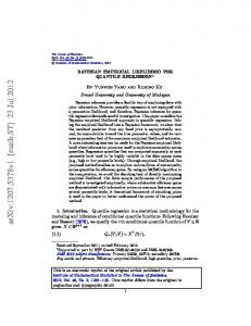
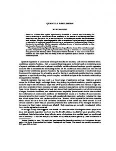
non-retail business acres per town (INDUS), a factor indicating whether tract borders Charles River (CHAS), nitric oxides concentration (parts per 10 million) per town (NOX), average numbers of rooms per dwelling (RM), proportions of owner-occupied units built prior to 1940 (AGE), weighted distances to five Boston employment centers (DIS), index of accessibility to radial highways per town (RAD), full-value propertytax rate per USD 10,000 per town (TAX), pupil-teacher ratios per town (PTRATIO), transformed African American population proportion (B) and percentage values of lower status population (LSTAT). Similar as in Section 3, we consider three choices of θ, 0.1, 0.3 and 0.5. Also, we run 10-fold cross-validation to evaluate the performance of the four methods under the check-loss criterion (1). The prior specifications are the same as those in Section 3, a = b = c = d = 0.1 for BQR.L and a = b = c1 = d1 = c2 = d2 = 0.1 for BQR.EN. The results are summarized in Table 8 and show that the Bayesian quantile regression methods perform uniformly better than the lasso and EN for all selected quantiles, and similarly to QR and QR-L. Again, as mentioned in the discussion of Tables 1, 2 and 3, the performance of QR-L drops when θ changes from 0.5 and 0.3 to 0.1. Also, instead of comparing the check loss, we can look at the point and interval estimations for the parameters. These are shown in Figures 1 through 3. As there are too many estimators in a plot, we add a slight horizontal shift to the estimators given by BQR.L and BQR.EN to make it more readable. Note that the Bayesian methods can easily provide the interval estimations while the frequentist methods usually do not have simply implemented interval estimators. From these figures we can see that the four quantile regression based methods tends to behave similarly while lasso and EN also behave similarly. Also, among the four quantile regression based methods, QR-L tends to behave more differently from the other three methods. This difference is more apparent when θ = 0.1 as there are more QR-L estimators lying outside the 95% credible intervals of BQR.L and BQR.EN.
Li, Q., Xi, R. and Lin, N.
17
BQR.L BQR.EN lasso EN QR QR−L
0.00 −0.20
−0.15
−0.10
−0.05
estimates
0.05
0.10
0.15
theta=0.5
2
4
6
8
10
12
14
predictor index
Figure 1: The estimates of the predictor effects for the Boston Housing data using different methods. The given quantile is θ = 0.5. The 95% credible intervals given by BQR.L and BQR.EN are also plotted.
18
BQR
BQR.L BQR.EN lasso EN QR QR−L
0.00 −0.20
−0.15
−0.10
−0.05
estimates
0.05
0.10
0.15
theta=0.3
2
4
6
8
10
12
14
predictor index
Figure 2: The estimates of the predictor effects for the Boston Housing data using different methods. The given quantile is θ = 0.3. The 95% credible intervals given by BQR.L and BQR.EN are also plotted.
Li, Q., Xi, R. and Lin, N.
19
BQR.L BQR.EN lasso EN QR QR−L
0.00 −0.20
−0.15
−0.10
−0.05
estimates
0.05
0.10
0.15
theta=0.1
2
4
6
8
10
12
14
predictor index
Figure 3: The estimates of the predictor effects for the Boston Housing data using different methods. The given quantile is θ = 0.1. The 95% credible intervals given by BQR.L and BQR.EN are also plotted.
20
5
BQR
Conclusion and Discussion
In this paper, we propose the Bayesian regularized quantile regression and treat generically three different types of penalties, lasso, elastic net and group lasso. Bayesian hierarchical models are developed for each regularized quantile regression problem and Gibbs samplers are built to solve the model efficiently. Simulation studies and real data examples show that Bayesian regularized quantile regression methods behave more satisfactory compared with current existing non-Bayesian regularized quantile regression methods. In particular, as counterparts to each other, BQR.L behaves better than QR-L. One of the most valued advantages of quantile regression is its model robustness in the sense that it makes no distributional assumption to the error term other than its quantile. However, in the parametric Bayesian quantile regression framework, a common practice is to assume the error to have the skewed Laplace distribution (2). While this may cause some concern on losing the nonparametric nature of quantile regression, our results show that the Bayesian methods are quite insensitive to this assumption and behave well for data generated from other distributions. One issue we found in the numerical studies is that, compared to the Bayesian methods, the performance of QR-L often deteriorates for extreme quantiles, such as θ = 0.1. It is worth future exploration to explain this phenomenon. Another future direction is to develop Bayesian regularization for multiple quantiles. Zou and Yuan (2008a,b) considered regularized quantile regression models for a finite number of quantiles. Our Bayesian formulation shall extend naturally to this context by imposing suitable functional priors on the coefficients.
Appendix A. The Gibbs sampler for the lasso regularized quantile regression Let β −k be the parameter vector β excluding the component βk , s−k be the variable ˜−i be the variable z ˜ excluding the component z˜i . s excluding the component sk and z ˜, β, s, τ, η 2 ) in the Denote X = (x1 , · · · , xn ). Then, the conditional distribution f (y|X, z lasso regularized quantile regression is
˜, β, s, τ, η 2 ) = f (y|X, z =
{ } 1 (yi − xTi β − ξ1 z˜i )2 √ exp − 2τ −1 ξ22 z˜i 2πτ −1 ξ22 z˜i i=1 } n { n 1 ∑ (yi − xTi β − ξ1 z˜i )2 ∏ 1 √ . exp − −1 ξ 2 z 2 i=1 τ −1 ξ22 z˜i 2πτ 2 ˜i i=1 n ∏
Li, Q., Xi, R. and Lin, N.
21
˜−i , β, s, τ, η 2 ) is The full conditional distribution f (˜ zi | X, y, z ˜−i , β, s, τ, η 2 ) ∝ f (y|X, z ˜, β, s, τ, η)π(˜ f (˜ zi | X, y, z zi |τ ) { } 1 (yi − xTi β − ξ1 z˜i )2 exp(−τ z˜i ) ∝ √ exp − 2τ −1 ξ22 z˜i z˜i { [( 2 ) ]} 1 1 τ ξ1 τ (yi − xTi β)2 −1 ∝ √ exp − . + 2τ z ˜ + z ˜ i i 2 ξ22 ξ22 z˜i Thus, the full conditional distribution of z˜i is a generalized inverse Gaussian distribution. ˜, β, s−k , τ, η 2 ) of sk is The full conditional distribution f (sk | X, y, z ( ) ( η2 ) 1 β 2 η2 ˜, β, s−k , τ, η 2 ) ∝ √ f (sk | X, y, z exp − k exp − sk 2sk 2 2 2πsk { } [ ] 1 1 ∝ √ exp − η 2 sk + βk2 s−1 . k sk 2 ˜, β, s−k , τ, η 2 ) is then again a generalized inverse GausThe full conditional f (sk | X, y, z sian distribution. Now we consider the full conditional distribution of βk which is given by ˜, β −k , s, τ, η 2 ) f (βk | X, y, z
˜, β, s, τ, η)π(βk | sk ) ∝ f (y|X, z { } n ( 1 ∑ (yi − xTi β − ξ1 z˜i )2 β2 ) ∝ exp − exp − k 2 −1 2 i=1 τ ξ2 z˜i 2sk [( ∑ ) { n n ∑ τ y˜ik xik ]} 1 τ x2ik 1 2 + βk , β − 2 ∝ exp − 2 ξ 2 z˜ sk k ξ22 z˜i i=1 2 i i=1 ∑p ∑n ˜k−2 = τ ξ2−2 i=1 x2ik z˜i−1 + where xi = (xi1 , · · · , xip )T and y˜ik = yi −ξ1 z˜i − j=1,j̸=k xij βj . Let σ ∑ n s−1 ˜k = σ ˜k2 τ ξ2−2 i=1 y˜ik xik z˜i−1 . Then the full conditional distribution is just the k and µ normal distribution N (˜ µk , σ ˜k2 ). The full conditional distribution of τ is ˜, β, s, η 2 ) f (τ | X, y, z
˜, β, s, τ, η)π(˜ ∝ f (y|X, z z | τ )π(τ ) { } n n ∑ ∑ (yi − xTi β − ξ1 z˜i )2 n 1 ∝ τ n/2 exp − τ exp(−τ z˜i )τ a−1 exp(−bτ ) 2 i=1 τ −1 ξ22 z˜i i=1 ) ]} { [∑ n ( T 2 (yi − xi β − ξ1 z˜i ) a+3n/2−1 ∝ τ exp − τ + z˜i + b . 2ξ22 z˜i i=1
That is, the full conditional distribution of τ is a Gamma distribution. At last, the full conditional distribution of η 2 is ˜, β, s, τ ) f (η 2 | X, y, z
∝ π(s | η 2 )π(η 2 ) p ∏ ( η 2 )( )c−1 η2 exp − sk η 2 exp(−dη 2 ) ∝ 2 2 k=1
∝
p ( 2 )p+c−1 { (∑ )} η exp − η 2 sk /2 + d . k=1
22
BQR
The full conditional distribution of η 2 is again a Gamma distribution.
B. Calculation of C(η1 , η2 ) and the Gibbs sampler for quantile regression with the elastic net penalty B.1 Calculation of C(η1 , η2 ) in (11) Before putting priors on η1 and η2 , let us first calculate the quantity C(η1 , η2 ). By (8), we have η1 exp{−η1 |βk | − η2 βk2 } 2 ∫ ∞ } η2 ( −η12 ) { 1 β2 √ = C(η1 , η2 ) exp − k − η2 βk2 1 exp sk dsk 2sk 2 2 2πsk 0 ∫ ∞ { 1 + 2η2 sk 2 } η12 ( −η12 ) (1 + 2η2 sk )−1/2 √ = C(η1 , η2 ) exp − βk exp sk dsk . 2sk 2 2 2πsk /(1 + 2η2 sk ) 0
π(βk | η1 , η2 ) = C(η1 , η2 )
Let tk = 1 + 2η2 sk . Then we have ∫
∞
π(βk | η1 , η2 ) = C(η1 , η2 ) 1
Since ∫
∞
−∞
∫∞ −∞
{
−1/2
tk
√ exp 2π(tk − 1)/(2η2 tk )
( )−1 } 2 { −η12 } 1 tk − 1 η1 − βk2 exp (tk − 1) dtk . 2 2η2 tk 4η2 4η2
π(βk | η1 , η2 )dβk = 1, by Fubini’s theorem, we have ∫
π(βk | η1 , η2 )dβk
∞
{ −η12 } η12 exp (tk − 1) dtk 4η 4η 2 2 1 ( 2 )1/2 ∫ ∞ 2 η1 η t−1/2 exp(−t)dt = 1. = C(η1 , η2 ) exp{ 1 } 4η2 4η2 4−1 η12 η2−1
= C(η1 , η2 )
−1/2
tk
∫∞ Notice that 4−1 η2 η−1 t−1/2 exp(−t)dt = Γ(1/2, 4−1 η12 η2−1 ) is the upper incomplete 1 2 gamma function. Therefore, we have C(η1 , η2 ) = Γ
−1
(
η2 1/2, 1 4η2
)(
η12 4η2
)−1/2
{ } η12 exp − . 4η2
B.2 The Gibbs sampler for quantile regression with the elastic net penalty The full conditional distributions of z˜i and τ are∑ again the same as in the lasso ∑nregularp ized quantile regression case. Let y˜ik = yi −ξ1 z˜i − j=1,j̸=k xij βj , σ ˜k−2 = τ ξ2−2 i=1 x2ik z˜i−1 + ∑n 2η2 tk (tk − 1)−1 and µ ˜k = σ ˜k2 τ ξ2−2 i=1 y˜ik xik z˜i−1 . Then, similar to the lasso regularized ˜, β −k , t, τ, η12 , η2 ) quantile regression case, we can show that the full conditional f (βk | X, y, z 2 of βk is the normal distribution N (˜ µk , σ ˜k ).
Li, Q., Xi, R. and Lin, N.
23
The full conditional distribution of tk − 1 is ˜, β, t−k , τ, η˜1 , η2 ) f (tk − 1 | y, X, z
∝ ∝
{ 1 exp − tk − 1 { 1 √ exp − tk − 1 √
( )−1 } { } 1 tk − 1 βk2 exp − η˜1 tk I(tk > 1) 2 2η2 tk [ ]} 1 2η2 βk2 2˜ η1 (tk − 1) + I(tk − 1 > 0). 2 tk − 1
Therefore, the full conditional distribution of tk − 1 is a generalized Gaussian distribution. The full conditional distribution of η˜1 is ˜, β, t, τ, η2 ) f (˜ η1 | X, y, z
∝ η˜1c1 −1 exp(−d1 η˜1 )
p ∏
Γ−1 (1/2, η˜1 )˜ η1
1/2
k=1
∝ Γ
−p
(1/2,
p/2+c1 −1 η˜1 )˜ η1
{ exp
{ } exp − η˜1 tk
[ ]} p ∑ − η˜1 d1 + tk . k=1
The full conditional of η2 is ˜, β, t, τ, η˜1 ) f (η2 | X, y, z
{
( )−1 } 1 tk − 1 exp − exp(−d2 η2 ) ∝ βk2 2 2η2 tk k=1 )} { ( p ∑ p/2+c2 −1 tk (tk − 1)−1 βk2 . ∝ η2 exp − η2 d2 + η2c2 −1
p ∏
1/2 η2
k=1
The full conditional of η2 is again a Gamma distribution.
C. The Gibbs sampler for the group lasso regularized quantile regression Let β −g be the parameter vector β excluding the component vector β g . It is easy to see that the full conditional distributions of z˜i and τ are the same as in the lasso regularized quantile regression. The full conditional distribution of sg is ˜, β, s−k , τ, η 2 ) ∝ f (sg | y, X, z ∝ ∝
π(β g |sg )π(sg |η 2 ) { 1 ( )−1 } (dg −1)/2 ( −η 2 ) g /2 s−d exp − β Tg sg Kg−1 β g sg exp sg g 2 2 ] 1[ }. exp{− η 2 sg + β Tg Kg β g s−1 s−1/2 g g 2
That is, the full conditional distribution of sg is again a generalized inverse Gaussian distribution. The full conditional distribution of β g is ˜, β −g , s, τ, η 2 ) f (β g | X, y, z
˜, β, s, τ, η)π(β g | sg ) ∝ f (y|X, z ∑G { } n { 1 ( ) } 1 ∑ (yi − k=1 xTik β k − ξ1 z˜i )2 ∝ exp − exp − β Tg s−1 g Kg β g . 2 −1 2 i=1 τ ξ2 z˜i 2
24
BQR
Let y˜ig = yi −
∑G k=1,k̸=g
xTik β k − ξ1 z˜i . Then, we have {
˜, β −g , s, τ, η ) f (β g | X, y, z 2
} n { 1 ( ) } yig − xTig β g )2 1 ∑ (˜ ∝ exp − exp − β Tg s−1 g Kg β g 2 i=1 τ −1 ξ22 z˜i 2 [ ( { ) ]} n n ∑ ∑ 1 −2 −1 T −2 −1 T ∝ exp − βTg s−1 K + τ ξ z ˜ x x β − 2τ ξ z ˜ y ˜ x β . g ig ig ig ig g g 2 2 i i g 2
−2 ∑n
i=1
−2 ∑n
˜ −1 = s−1 Kg + τ ξ ˜ gτ ξ ˜g = Σ Let Σ ˜i−1 xig xTig and µ ˜i−1 y˜ig xig . The full g g 2 2 i=1 z i=1 z ˜ g ). The full conditional distribution of η 2 is given by ˜ g, Σ conditional of β g is then N (µ ˜, β, s, τ ) f (η 2 | X, y, z
∝
G ∏
π(sg | η 2 )π(η 2 )
g=1
∝ ∝
G ∏ ( 2 )(dg +1)/2 ( −η 2 )( 2 )c−1 sg η exp(−dη 2 ) η exp 2 g=1 G ( 2 )(p+G)/2+c−1 { (∑ )} η exp − η 2 sg /2 + d . g=1
The full conditional distribution of η 2 is again a Gamma distribution.
References Andrews, D. F. and Mallows, C. L. (1974). “Scale Mixtures of Normal Distributions.” Journal of the Royal Statistical Society, Ser. B, 36: 99–102. Bae, K. and Mallick, B. (2004). “Gene Selection Using a Two-Level Hierarchical Bayesian Model.” Bioinformatics, 20: 3423–3430. Bakin, S. (1999). “Adaptive Regression and Model Selection in Data Mining Problems.” PhD thesis, Australian National University, Canberra. Fan, J. and Li, R. (2001). “Variable Selection via Nonconcave Penalized Likelihood and Its Oracle Properties.” Journal of the American Statistical Association, 96: 1348– 1360. Geraci, M. and Bottai, M. (2007). “Quantile Regression for Longitudinal Data Using the Asymmetric Laplace Distribution.” Biostatistics, 8: 140–154. Hanson, T. and Johnson, W. (2002). “Modeling Regression Error with a Mixture of P´olya trees.” Journal of the American Statistical Association, 97: 1020–1033. Harrison, D. and Rubinfeld, D. L. (1978). “Hedonic Prices and the Demand for Clean Air.” Journal of Environmental Economics and Management, 5: 81–102. Hjort, N. and Walker, S. (2009). “Quantile Pyramids for Bayesian Nonparametrics.” Annals of Statistics, 37: 105–131.
i=1
Li, Q., Xi, R. and Lin, N.
25
Jørgensen, B. (1982). Statistical Properties of the Generalized Inverse Gaussian Distribution, Lecture Notes in Statistics, volume 9. Springer-Verlag. Koenker, R. (2004). “Quantile Regression for Longitudinal Data.” Journal of Multivariate Analysis, 91: 74–89. — (2005). Quantile Regression. New York: Cambridge University Press. Koenker, R. and Bassett, G. W. (1978). “Regression Quantiles.” Economerrica, 46: 33–50. Kottas, A. and Gelfand, A. (2001). “Bayesian Semiparametric Median Regression Modeling.” Journal of the American Statistical Association, 96: 1458–1468. Kottas, A. and Krnjaji´c, M. (2009). “Bayesian Semiparametric Modeling in Quantile Regression.” Scandinavian Journal of Statistics, 36: 297–319. Kozumi, H. and Kobayashi, G. (2009). “Gibbs Sampling Methods for Bayesian Quantile Regression.” Technical report, Kobe University. Li, Y. and Zhu, J. (2008). “L1 -Norm Quantile Regression.” Journal of Computational and Graphical Statistics, 17: 163–185. Meier, L., van de Geer, S., and B¨ uhlmann, P. (2008). “The Group Lasso for Logistic Regression.” Journal of the Royal Statistical Society, Ser. B, 70(1): 53–71. Park, T. and Casella, G. (2008). “The Bayesian Lasso.” Journal of the American Statistical Association, 103: 681–686. R Development Core Team (2005). R: A language and environment for statistical computing. R Foundation for Statistical Computing, Vienna, Austria. URL http://www.R-project.org Reed, C., Dunson, D., and Yu, K. (2009). “Bayesian variable selection in quantile regression.” Technical report. Reed, C. and Yu, K. (2009). “An efficient Gibbs sampler for Bayesian quantile regression.” Technical report. Reich, B., Bondell, H., and Wang, H. (2009). “Flexible Bayesian Quantile Regression for Independent and Clustered Data.” Biostatistics. Doi:10.1093/biostatistics/kxp049. Tibshirani, R. (1996). “Regression Shrinkage and Selection via the Lasso.” Journal of the Royal Statistical Society, Ser. B, 58: 267–288. Tibshirani, R., Saunders, M., Rosset, S., Zhu, J., and Knight, K. (2005). “Sparsity and Smoothness via the Fused Lasso.” Journal of the Royal Statistical Society: Ser. B, 67: 91–108. Tsionas, E. (2003). “Bayesian Quantile Inference.” Journal of Statistical Computation and Simulation, 73: 659–674.
26
BQR
Walker, S. and Mallick, B. (1999). “A Bayesian Semiparametric Accelerated Failure Time Model.” Biometrics, 55: 477–483. Wang, H., Li, G., and Jiang, G. (2007). “Robust Regression Shrinkage and Consistent Variable Selection Through the LAD-Lasso.” Journal of Business & Economic Statistics, 25: 347–355. Wu, Y. and Liu, Y. (2009). “Variable Selection in Quantile Regression.” Statistica Sinica, 19: 801–817. Yu, K. and Moyeed, R. (2001). “Bayesian Quantile Regression.” Statistics & Probability Letters, 54: 437–447. Yuan, M. and Lin, Y. (2006). “Model Selection and Estimation in Regression with Grouped Variables.” Journal of the Royal Statistical Society, Ser. B, 68: 49–67. Zou, H. and Hastie, T. (2005). “Regularization and Variable Selection via the Elastic Net.” Journal of the Royal Statistical Society, Ser. B, 67: 301–320. Zou, H. and Yuan, M. (2008a). “Composite Quantile Regression and The Oracle Model Selection Theory.” Annals of Statistics, 36: 1108–1126. — (2008b). “Regularized Simultaneous Model Selection in Multiple Quantiles Regression.” Computational Statistics & Data Analysis, 52: 5296–5304.