Bayesian Statistics ... belief. In general, the Bayes factor depends on the prior: B
= ..... z. −(m+3)/2 e. −1/z dz [ where z = 2w x2 +mS2. ∝ (x. 2. +mS. 2. ) −(m+1)/2.
Bayesian Statistics Course notes by Robert Pich´e, Tampere University of Technology based on notes by Antti Penttinen, University of Jyv¨askyl¨a version: March 9, 2009
8
Hypothesis Testing
As pointed out in chapter 4, Bayesian hypothesis testing is straightforward. For a hypothesis of the form Hi : θ ∈ Θi , where Θi is a subset of the parameter space Θ, we can compute the prior probability πi = P(Hi ) = P(θ ∈ Θi ) and the posterior probability pi = P(Hi | y) = P(θ ∈ Θi | y). Often, there are only two hypotheses, the “null hypothesis” H0 and its logical negation H1 : θ 6∈ Θ0 , called the “alternative hypothesis”. The hypothesis with the highest probability can be chosen as the “best” hypothesis; a more sophisticated choice can be made using Decision Theory (to be discussed in section 14). Two hypotheses can be compared using odds. The posterior odds in favour of H0 against H1 given data y are given by the ratio p0 P(H0 | y) P(H0 ) P(y | H0 ) = = × . p1 P(H1 | y) P(H1 ) P(y | H1 ) | {z } | {z } B
π0 /π1
The number B, called the Bayes factor, tells us how much the data alters our prior belief. In general, the Bayes factor depends on the prior: R
R
P(H0 | y)/π0 Θ p(θ | y) dθ /π0 Θ p(y | θ )p(θ )/π0 dθ . B= =R 0 =R 0 P(H1 | y)/π1 Θ1 p(θ | y) dθ /π1 Θ1 p(y | θ )p(θ )/π1 dθ However, when the parameter space has only two elements, the Bayes factor is the likelihood ratio p(y | θ0 ) B= . p(y | θ1 ) which does not depend on the choice of the prior. This interpretation applies in the following example. Example: Transmission of hemophilia The human X chromosome carries a gene that is essential for normal clotting of the blood. The defect in this gene that is responsible for the blood disease hemophilia is recessive: no disease develops in a woman at least one of whose X chromosomes has a normal gene. However, a man whose X chromosome has the defective gene develops the disease. As a result, hemophilia occurs almost exclusively in males who inherit the gene from non-hemophiliac mothers. Great Britain’s Queen Victoria (pictured here) carried the hemophilia gene, and it was transmitted through her daughters to many of the royal houses of Europe. 1
Question. Alice has a brother with hemophilia, but neither she, her parents, nor her two sons (aged 5 and 8) have the disease. What is the probability that she is carrying the hemophilia gene? Solution. Let H0 : Alice does not carry the hemophilia gene, and H1 : she does. The X chromosome that Alice inherited from her father does not have the defective gene, because he’s healthy. We know that Alice’s mother has one X chrosomome with the defective gene, because Alice’s brother is sick1 and her mother is healthy. The X chromosome that Alice inherited from her mother could be the good one or the bad one; let’s take P(H0 ) = P(H1 ) = 21 as our prior, that is, we assume prior odds to be 1 to 1. Let Y denote the fact that Alice’s two sons are healthy. Because the sons are not identical twins, we can assume P(Y | H1 ) =
1 1 1 · = , 2 2 4
P(Y | H0 ) = 1.
The posterior probability is then P(H1 |Y ) =
P(Y | H1 )P(H1 ) = P(Y | H1 )P(H1 ) + P(Y | H0 )P(H0 )
1 4
·
1 1 4·2 1 1 2 +1· 2
1 = , 5
and P(H0 |Y ) = 1 − 15 = 45 . The posterior odds in favour of H0 against H1 are 4 to 1, much improved (Bayes factor B = 4) compared to the prior odds. � A one-sided hypothesis for a continuous parameter has a form such as H0 : θ ≤ θ0 , where θ0 is a given constant. This could represent a statement such as “the new fertilizer doesn’t improve yields”. After you compute the posterior probability p0 = P(H0 | y) = P(θ ≤ θ0 | y) =
Z θ0
p(θ | y) dθ ,
−∞
you can make straightforward statements such as “The probability that θ ≤ θ0 is p0 ”, or “The probability of that θ > θ0 is 1 − p0 ”. Some practicioners like to mimic Frequentist procedures and choose beforehand a “significance level” α (say, α = 5%), and then if p0 < α they “reject H0 (and accept H1 ) at the α level of significance”. This is all rather convoluted, however, and as we shall see in section 14, a systematic approach should be based on Decision Theory. Simply reporting the probability value p0 is more direct and informative, and usually suffices. A two-sided hypothesis of the form H0 : θ = θ0 might be used to model statements such as “the new fertilizer doesn’t change yields.” In Bayesian theory, such a “sharp” hypothesis test with a continuous prior pdf is pointless because it is always false: P(θ = θ0 | y) =
Z θ0
p(θ | y) dθ =
θ0
Z θ0
p(y | θ )p(θ ) dθ = 0.
θ0
Thus it would seem that the question is not a sensible one. It nevertheless arises fairly often, for example when trying to decide whether to add or remove terms to a regression model. How, then, can one deal with such a hypothesis? 1 For
simplicity, we neglect the fact that hemophilia can also develop spontaneously as a result of a mutation.
2
• One could test whether θ0 lies in some credibility interval Cε . However, this isn’t a Bayesian hypothesis test. • A Bayesian hypothesis test consists of assigning a prior probability π0 > 0 to the hypothesis H0 : θ = θ0 , yielding a prior that is a mixture of discrete pmf and continuous pdf. We shall discuss this further in section 13.
9
Simple Multiparameter Models
Often, even though one may need many parameters to define a model, one is only interested in a few of them. For example, in a normal model with unknown mean and variance yi | µ, σ 2 ∼ Normal(µ, σ 2 ), one is usually interested only in the mean µ. The uninteresting parameters are called nuisance parameters, and they can simply be integrated out of the posterior to obtain marginal pdfs of the parameters of interest. Thus, denoting θ = (θ1 , θ2 ), where θ1 is the vector of parameters of interest and θ2 is the vector of ‘nuisance’ parameters, we have p(θ1 | y) =
Z
p(θ | y) dθ2 .
This marginalisation integral can also be written as p(θ1 | y) =
Z
p(θ1 | θ2 , y)p(θ2 | y) dθ2 ,
(1)
which expresses θ1 | y as a mixture of conditional posterior distributions given the nuisance parameters, weighted by the posterior density of the nuisance parameters. This explains why the posterior pdf for the parameters of interest is generally more diffuse than p(θ1 | θ2 , y) for any given θ2 .
9.1
Two-parameter normal model
Consider a normal model with unknown mean and variance, that is, yi | µ, σ 2 ∼ Normal(µ, σ 2 ) with y = y1 , . . . , yn conditionally independent given µ, σ 2 . The likelihood is then 2
p(y | µ, σ ) ∝ σ
1 n 2 −n − 2σ 2 ∑i=1 (yi −µ)
e
=σ
−n −
e
2 +∑n (y −y) 2 n(y−µ) ¯ i=1 i ¯ 2σ 2
where y¯ = 1n ∑ni=1 yi is the sample mean and s2 = variance. We assume the following prior information:
e
2 +(n−1)s2 n(y−µ) ¯ 2σ 2
1 n ¯2 n−1 ∑i=1 (yi − y)
is the sample
=σ
−n −
• µ and σ 2 are independent. • p(µ) ∝ 1. This improper distribution expresses indifference about the location of the mean, because a translation of the origin µ 0 = µ + c gives the same prior. • p(σ ) ∝ σ1 . This improper distribution expresses indifference about the scale of the standard deviation, because a scaling σ 0 = cσ gives the same prior p(σ 0 ) = p(σ ) dσ / dσ 0 ∝ σ10 . Equivalently, we can say that this improper distribution expresses indifference about the location of log(σ ), because a ) 1 flat prior p(log(σ )) ∝ 1 corresponds to p(σ ) = d log(σ dσ p(log(σ )) ∝ σ . The corresponding prior distribution for the variance is p(σ 2 ) ∝ σ12 . 3
,
With this prior and likelihood, the joint posterior pdf is −( n2 +1)
p(µ, σ 2 | y) ∝ (σ 2 )
− e
(n − 1)s2 + n(y¯ − µ)2 2σ 2 ,
(2)
The posterior mode can be found as follows. The mode’s µ value is y¯ because of the symmetry about µ = y. ¯ Then, denoting v = log σ and A = (n − 1)s2 + n(y¯ − µ)2 , we have log p(µ, σ 2 | y) = −(n + 2)v − 12 Ae−2v Differentiating this with respect to v, equating to zero, and solving gives n+2 . A
e−2v = Substituting ev = σ and µ = y¯ gives
mode(µ, σ 2 | y) = (y, ¯
n−1 2 s ). n+2
(3)
The marginal posterior pdf of σ 2 is obtained by integrating over µ: 2
p(σ | y) =
Z ∞ −∞
p(µ, σ 2 | y) dµ
2 −( n2 +1) −
= (σ )
e
(n−1)s2 2σ 2
Z ∞ n(µ−y) ¯2 − 2σ 2
e
−∞
√ {z 2
|
dµ }
2πσ /n
∝ (σ 2 )−(
n+1 2 )
−
e
(n−1)s2 2σ 2
,
n−1 2 that is, σ 2 | y ∼ InvGam( n−1 2 , 2 s ), for which
E(σ 2 | y) =
n−1 2 s , n−3
mode(σ 2 | y) =
n−1 2 s , n+1
V(σ 2 | y) =
2(n − 1)2 s4 . (n − 3)2 (n − 5)
Notice that the mode of the marginal posterior is different from (a bit larger than) the joint posterior mode’s σ 2 value given in (3). The following general result will be useful. Lemma 1 If x | w ∼ Normal(0, w) and w ∼ InvGam( m2 , m2 S2 ) then dard Student-t distribution with m degrees of freedom.
x S
∼ tm , a stan-
Proof: The marginal pdf is Z ∞
p(x) =
p(x | w)p(w) dw ∝
Z
1
x2
m
mS2
w− 2 e− 2w w−( 2 +1) e− 2w dw
0
� =
x2 + mS2 2
�−(m+1)/2 Z
z−(m+3)/2 e−1/z dz
[ where z =
∝ (x2 + mS2 )−(m+1)/2 [ integral of an inverse-gamma pdf � �−(m+1)/2 x2 ∝ 1+ 2 .� mS
4
2w x2 + mS2
2
µ− √y¯ | σ 2 , y ∼ Normal(0, σ 2 ). From (2) we have µ | σ 2 , y ∼ Normal(y, ¯ σn ), so that 1/ n
Then by Lemma 1 we have E(µ | y) = y, ¯
µ− √y¯ | y ∼ tn−1 , s/ n
2
that is, µ | y ∼ tn−1 (y, ¯ sn ), and
mode(µ | y) = y, ¯
V(µ | y) =
n − 1 s2 . n−3 n
The Student-t distribution roughly resembles a Normal distribution but has heavier tails. This marginal posterior distribution has the same mean as that of the posterior µ | y ∼ Normal(y, ¯ nv ) that we found in section 5.1 for the one-parameter normal model with known variance v and uniform prior p(µ) ∝ 1. Next, we find the posterior predictive distribution. The model is y˜ | µ, σ 2 ∼ Normal(µ, σ 2 ) (conditionally independent of y given µ, σ 2 ). Because y− ˜ µ | σ 2, y ∼ 2 Normal(0, σ 2 ) and µ | σ 2 , y ∼ Normal(y, ¯ σn ) are independent given σ 2 , y, we have ˜ y¯ 2 2 y˜ | σ 2 , y ∼ Normal(y, ¯ (1 + n1 )σ 2 ), that is, (1+y− 1 1/2 | σ , y ∼ Normal(0, σ ). Then by ) Lemma 1, we obtain
y− ˜ y¯ (1+ n1 )1/2 s
E(y˜ | y) = y, ¯
n
∼ tn−1 , that is, y˜ | y ∼ tn−1 (y, ¯ (1 + 1n )s2 ), for which
mode(y˜ | y) = y, ¯
V(y˜ | y) =
n−1 1 (1 + )s2 . n−3 n
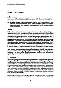
The formulas derived in this section can be generalised by considering families of conjugate prior distributions. However, the formulas and their derivations do not add much insight to the results already derived. We proceed instead to look at how a two-parameter normal model can be analysed using numerical simulation. Example: Two-parameter normal model for Cavendish’s data We have n = 23, y¯ = 5.4848, and s2 = (0.1924)2 = 0.0370. With the prior p(µ, σ 2 ) = 1/σ 2 , the posterior pdf’s are:
p(µ, σ 2 | y)
p(µ|y)
300
0.08
5.6 5.4 5.5
0.04 2
5.4
µ
σ
0.04
σ
5.6
p( y˜|y)
p(σ 2 |y)
0
5.5
µ
5
0.08 2
y˜
6
mode(µ, σ 2 | y) = (5.4848, 0.0326), E(µ | y) = 5.4848, mode(µ | y) = 5.4848, V(µ | y) = 0.0018, E(σ 2 | y) = 0.0407, mode(σ 2 | y) = 0.0339, V(σ 2 | y) = 1.84 · 10−4 , E(y˜ | y) = 5.4848, mode(y˜ | y) = 5.4848, V(y˜ | y) = 0.0425. For a WinBUGS model, we assume µ and σ 2 to be independent a priori. As in section 4.2, we choose µ ∼ Normal(5, 0.5). Our prior for σ 2 is based on 5
the judgement that σ 2 ≈ 0.04 ± 0.02. Assuming σ 2 ∼ InvGam(α, β ) and solving E(σ 2 ) = 0.04 and V(σ 2 ) = 0.022 for α and β , we obtain σ 2 ∼ InvGam(6, 0.2). The corresponding prior distribution for the precision τ = 1/σ 2 is τ ∼ Gamma(6, 0.2).
p(σ 2 )
0
0.04
0.08
σ2
The WinBUGS model is model { for (i in 1:n) { y[i] ∼ dnorm(mu,tau) } mu ∼ dnorm(5,2) tau ∼ dgamma(6,0.2) sigma2