econometrics Article
Between Institutions and Global Forces: Norwegian Wage Formation Since Industrialisation † Ragnar Nymoen 1,2 1 2
†
Department of Economics, University of Oslo, POB 1095 0317 Oslo, Norway;
[email protected]; Tel.: +47-22-855-148 Centre for Wage Formation at Economic Analysis, POB 0650, Oslo, Norway Paper presented at the workshop Macroeconomics and Policy Making, arranged in honour of Asbjørn Rødseth, 18 May, 2016, by the Department of Economics, University of Oslo. Thanks to Olav Bjerkholt for comments, and for showing me the article written by Frisch about “rational wage policies”, and the correspondence with Haavelmo that it led to. Discussions at the Workshop in econometrics at Statistics Norway, 21 October 2016, were also very useful, thanks to the participants. Thanks also to Jan Morten Dyrstad, David F. Hendry , Steinar Holden, Tord S. Krogh and Mikkel Myhre Walbækken for important comments and suggestions. Finally, thanks to the editors and to two anonymous referees for their comments, both critical and constructive. The numerical results in this paper were obtained by the use of OxMetrics 7/PcGive 14 and Eviews 9.5.
Academic Editors: Gilles Dufrénot, Fredj Jawadi and Alexander Mihailov Received: 31 August 2016; Accepted: 13 December 2016; Published: 12 January 2017
Abstract: This paper reviews the development of labour market institutions in Norway, shows how labour market regulation has been related to the macroeconomic development, and presents dynamic econometric models of nominal and real wages. Single equation and multi-equation models are reported. The econometric modelling uses a new data set with historical time series of wages and prices, unemployment and labour productivity. Impulse indicator saturation is used to achieve robust estimation of focus parameters, and the breaks are interpreted in the light of the historical overview. A relatively high degree of constancy of the key parameters of the wage setting equation is documented, over a considerably longer historical time period than earlier studies have done. The evidence is consistent with the view that the evolving system of collective labour market regulation over long periods has delivered a certain necessary level of coordination of wage and price setting. Nevertheless, there is also evidence that global forces have been at work for a long time, in a way that links real wages to productivity trends in the same way as in countries with very different institutions and macroeconomic development. Keywords: wage formation; economic history of Norway; structural breaks; labour market regulation; econometric models of inflation JEL Classification: C22; C31; E23; E24; E31; J38; J50; J51; N14; N34; O52
In the days of Manchester liberalism, the wage contract was a matter between the individual worker and employer. Any “wage policies”, either by the society or by the organizations, were non-existent. Luckily, this has been changed. Ragnar Frisch (Arbeiderbladet 30 August 1945) [1]. 1. Introduction The newspaper article by professor Ragnar Frisch, where the quotation is taken from, continued with the observation that one of the (“lucky”) things that had happened was that “wage policies”
Econometrics 2017, 5, 6; doi:10.3390/econometrics5010006
www.mdpi.com/journal/econometrics
Econometrics 2017, 5, 6
2 of 54
had come to take a central place in economic policy thinking and practice, alongside monetary and fiscal policy 1 . Frisch put this down to the increased political importance of redistribution and “social justice”. However, even more importantly, he cited the fact that the general wage level is one of the main factors that determine the activity level in a capitalist industrialised economy, both as a cost factor for producers, and as a main determinant of aggregate demand in the economy. In that way, Frisch wrote, the general wage level had become a central variable in the “most important of all economic processes” 2 . Frisch’s main motive for writing the newspaper article may have been to present some ideas about what he called a “rational wage policy” that would make it possible to reconcile full employment and a certain stability of the price level. In this Frisch was not alone. For example, American and British economists commented on the challenges and dilemmas that the western economies would face during the post war period, as inflation and international competitiveness replaced mass unemployment as the main problems for macroeconomic policy makers. Frisch was clearly looking for a conceptualization, and an operationalization, of a wage norm for the Norwegian economy as a whole. Yet he did not give attention to the important developments towards practical collective labour market regulation that had taken place in the early decades of the 20th century. It was those developments, which we review in Section 2.5, not Frisch’s theoretical formulations, that came to provide the operational definition of the wage norm, which became a mainstay of the system of wage formation during the whole post-war period. Nevertheless, there is nothing in this that would have reduced the relevance of Frisch’s timely identification of wage setting as one of the most important economic processes of the modern market based economy. This has been confirmed time and time again, not only by the (ebbing and flowing) stream of academic offerings in the field, but even more by the many political involvements and initiatives that have been launched over the years, some of them ill-fated, others more successful. The continued relevance of wage setting is also the motivation of this paper, where I attempt to give econometric treatment to the formation of the general wage level in Norway over a period of 115 years. Since industrialisation started very late in the 1800s in Norway, the sample period therefore covers the epoch with an industrialised economy. In turn, because the organization among workers and firms happened in tandem with the growth of modern electricity based heavy industry, it meant that one premiss for collective labour market regulation was a reality already early in our sample period. Inevitably, another force established itself at it same time, and that was the economic laws of international product markets. Early in the century, nationwide collective agreements were struck in important manufacturing sectors for the first time 3 . The idea that industrial peace, not strife, was possible as a sort of normal situation in the labour market, seems to have motivated both union leaders and industrialists quite early in our data period. That did not mean that the days of industrial unrest were over though. The 1920s, and part of the 1930s, saw years when the number of working days lost in strikes and
1
2
3
Ragnar Frisch was professor at the University of Oslo from 1931 to 1965, a founder of The Econometric Society and was awarded the first Nobel Prize in economics in 1969. Frisch seems to have been deeply influenced by observing at close range the impact of deflationary policies in Norway in the 1920s and by the Great Depression in the 1930s. His scientific work was motivated by the need for social improvements as much as an intellectual interest, Bjerkholt (2014) [2] (p. 299) and Bjerkholt and Qin (2011) [3] (p. 11). All quotes from the newspaper article (and the correspondence that it led to) have been translated by the author. Frisch’s newspaper article is interesting also because it led to a correspondence with his pre-war assistant and colleague Trygve Haavelmo, who was still in USA, where he had been exiled during the war. Haavelmo opened by saying that he was “very interested in the problems” that Frisch had analysed in the article, and then went on to present a detailed note with comments (and improvements). Frisch, who wanted Haavelmo to come back to the University of Oslo, wrote back with enthusiasm and said that it was of the “greatest importance” that Haavelmo committed himself intellectually to this “all important field”, the theory of rational wage setting. See Olstad (2009) [4], in particular chapter 5, and the concluding chapter.
Econometrics 2017, 5, 6
3 of 54
lockouts were extremely high. However, these years can hardly be counted as normal in any sense of the word. The difficulties for the economy, and the strains on the political system, were enormous. Underlying the early development was a recognition among union leaders that international product markets and capitalist principles had certain consequences. For example: private owners’ right to organize and lead work, and that the firm’s profitability represented the basis for wage claims. As long as there was enough protection from unwanted competition in the labour market (which could undermine the ability to organise), competition and international trade in the product markets brought many benefits for trade union members. In this perspective, the system of wage setting was formed, and has been adapted under the influence of two strong forces: Domestic labour market institutions and global market forces. In order to avoid Frisch’s Manchester liberalism, collective bargaining had to become institutionalised. However, in order to become stable, labour market regulation in turn needed to be compatible with private ownership and with competitive product markets. This balancing act, between liberalised product markets and labour markets with enough protection from unwanted competition to sustain a system of collective bargaining, not only defined the development of wage setting in Norway. It was unavoidable and ubiquitous in western economies for most of the 20th century 4 . In Norway, the balancing act is still going on, centered around the consequences of liberalised labour market immigration from Europe during and after the financial crisis. From the perspective of the modeller of wage setting, there is an interesting side effect of this duality, namely that the forces of institutions and of markets have been present in the data over a long historical period. Hence, there may be an element of continuity in the data generation process, despite the variability and huge changes in individual years, and this motivates empirical modelling over the long sample. This study therefore starts with a review, in Section 2, of a century (plus) of economic history, focusing on labour market regulation and institutions. Section 3 recounts briefly the economic theory of wages, and I then specify a theoretical macro economic model that can be a relevant framework for empirical modelling. It is shown that the specified Incomplete Competition Model (ICM) has dynamic solutions that are qualitatively similar to the historical development of, for example, nominal and real wages, but also unemployment and the real exchange rate. The theoretical framework also contains the wage and price Phillips Curve Model (PCM) as a special case. These models represent different theoretical possibilities of wage-price coordination, especially when there is a target of near full unemployment, see Kolsrud and Nymoen (2014, 2015) [6,7]. The framework is therefore relevant for our empirical modelling project, which however requires identification and representation of structural breaks to achieve robust estimation of focus parameters, parameter constancy and identification, see Hendry (2017) [8]. Section 4 documents empirical coefficient constancy, and invariance, of the nominal wage setting equation over a considerably longer historical time period than earlier studies have done. The relationship is not (merely) a statistical relationship, it has a clear interpretation as an economic relationship showing that collective bargaining has been the main factor in wage formation. The econometric modelling results for wage formation, both single- and multiple-equation, also clarify methodological issues, and they have policy implications. They invalidate the still common way of obtaining estimates of a natural rate of unemployment by inverting the wage Phillips curve. Instead, equilibrium unemployment is defined by a multi-equation model of wages, domestic and foreign prices, productivity and the unemployment rate. The results therefore entail that empirical
4
Britain is an interesting case for historical comparison. At the time when the industrial unrest of the late 1960s was more of a nuisance than an unmanageable problem, Labour party minister Barbara Castle became frustrated by the unions’ lack of understanding that living in a liberalised market economy had consequences for how the unions could act. She mothered the ill fated White Paper In place of Strife in 1969, which in retrospect defined a turning point in the history of labour market regulation in Britain, see Sandbrook (2006) [5] (pp. 709–710).
Econometrics 2017, 5, 6
4 of 54
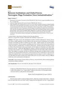
relevance suffers if the steady state of a medium term macro model is taken as exogenous, as the dynamic stochastic general equilibrium models (DSGEs) do. Another implication is that unions and firm owners’ organizations, through, for example, coordinated wage formation, can aid economic policy by making sure that inflation, labour market disputes, low mobility and low productivity growth do not become obstacles for the attainment of other important policy targets like full employment. However, the social partners cannot determine unemployment, or secure full employment, as some economists suggested would be their right role in a regime where the central bank supposedly takes care of the nominal path (wages and prices) of the economy, see, e.g., Norges Bank (2002) [9] (pp. 28,29), Isachsen (2008) [10] (p. 8). To this they do not have the instruments. The results of this investigation support that a much more concerted policy adjustment is required, and that this was well understood during the post-war period, but also that even this may not be enough, if the economy is hit by external shocks, or has to correct imbalances that have been allowed to build up over time. 2. A Century Plus of Labour Market Change The sample period for our empirical econometric analysis begins at the start of the 20th century and ends in 2015. However, the Norwegian economy of 1900 had a pre-history in the 1800s, which is relevant for understanding the development that took place in the first decade of our main sample period. I therefore first comment on some important trends of the last part of the 19th century, see Section 2.1. I then turn to the development after 1900, which was marked by the end of mass emigration and of the underemployment that it reflected, see Section 2.2. The other parts of the chapter, Sections 2.3–2.6, contain a presentation of the time series for unemployment and productivity, and discuss the development of labour market regulation and institutions. The dual, sometimes conflicting, developments towards product market deregulation and globalization, and a strong trait of collective regulation of the labour market, is a main theme. That section also gives the backdrop for the empirical modelling, including the assessment of the relevance of the economic theory of wages, see Section 3, which of course is central in the econometric models in Section 4. 2.1. The Norwegian Economy at the Start of the 20th Century At the start of the 20th century, Norway was barely an industrialised country. In 1900, almost half of the employment was in agriculture, forestry and fisheries. In comparison, only 11% worked in the primary sectors of the earlier industrialised UK economy, see Skoglund (2013) [11] and Lindsay (2000) [12]. Twenty-four percent of the employment was in manufacturing and other secondary industries, while it was 54% in the UK. Long periods of the previous century had been marked by low economic growth, stagnation in real wage growth, and by mass emigration, to North America in particular. As the graph in Figure 1 shows, emigration included three big waves with peaks in emigration rates above 1 percent of the population size. In Europe, only Ireland had higher emigration rates. Emigration was selective within cohorts, with many leaving who would have contributed to the Norwegian economy if given a chance, Bævre et al. (2001) [13]. There can be little doubt that the emigration to North America during the second half of the 1800s reflected a high degree of underemployment in Norway. It is also easy to imagine that the Norwegian unemployment rate early in the 20th century would have been considerably larger than 4.5 percent, if emigration had not been possible 5 . If we use ratios for the period 1903–1910, when we have data of emigration, employment and unemployment, the implied unemployment “without emigration” in 1900 becomes between 7% and 9% . Of course, this is only a crude interval, but it is nevertheless a reminder that the scale of
5
The number is for 1903 which is the earliest year with data, cf. Appendix A.
Econometrics 2017, 5, 6
5 of 54
emigration was large enough to affect the balance between supply and demand in the domestic labour market, see Søbye (2014) [14] (p. 107). 1.50
Emigration in percent of population
1.25
1.00
Years with net immigration
0.75
0.50
0.25
1850
1860
1870
1880
1890
1900
1910
1920
1930
1940
Figure 1. Emigration in percent of the Norwegian population. Source: Søbye (2014) [14] (Table 15).
The last 25–30 years of the 19th century nevertheless marked a time-shift. In 1900 the real wage was 67 percent higher than in 1870, which was a much better performance than earlier in the century. GDP per capita had grown by 38 percent over the same period 6 . 2.2. The End of Mass Emigration It is well known that emigrants often returned to Norway, and it is realistic to think that the propensity to re-immigrate increased during the 1920s, not to speak of in the 1930s, during the Great Depression in USA. In addition, many workers from Sweden came to several large construction and building works in Norway early in the 1900s. A boom in building and construction was a consequence of the first world war, and of a very accommodating monetary policy 7 . Also the government sector contributed to the demand for construction workers in these years, with 1919 and 1920 as particularly buoyant years, see Søbye (2014) [14] (p. 94). According to Søbye (2014) [14] (pp. 92–97), 1915 and 1916 (when gross emigration was in any case very low) may have been the first years with net immigration, and definitively 1917, when more than thirteen thousand immigrants were added to the Norwegian labour force 8 . High labour immigration continued until 1920. In 1921 labour immigration dropped sharply, and in 1922 or 1923 the situation had no doubt changed back to positive net emigration from Norway. However, in the period 1931 to 1940, net immigration again contributed to population growth in Norway. For example, Grytten (2008) [17] argues that the tens of thousands who returned to Scandinavia after the start of the Great Depression in USA, meant a significant increase in labour supply.
6 7
8
Fixed 1990 International Geary-Khamis dollars, Maddison project database: http://www.ggdc.net/maddison/ maddison-project/data.htm. Norway left the Gold standard in 1914, even though it was a neutral country with no war efforts to finance, cf. Lie (2012) [15] (pp. 32,33). Norges Bank’s monetary expansion during the first two years of the war was related to international trade flows. However, during the two last war years another part of the monetary expansion was result of credit to domestic borowers, Værholm and Øksendal (2010) [16]. There was more than 25,000 immigrants in total in 1917, while only 2500 left Norway, Søbye (2014) [14] (Tables 4 and 15).
Econometrics 2017, 5, 6
6 of 54
2.3. Unemployment and Productivity The boom during WW-I continued until 1919, but was stopped short in 1920 by a deflationary economic policy in the western European economies, notably the UK and Sweden, Norway’s most important trading partners. This policy was monitored by the central banks in order to decrease prices, and thereby increase the value of their currencies back to par gold values. Norway followed suit, and one of the deflationary consequences was the increase in the rate of unemployment seen in Figure 2. The gold-parity target was reached in 1928, but Norway, again following Bank of England’s example, left the gold standard in September 1931. Monetary policy came off the deflationary track that had been followed (with only a few stops) since 1920. Lowered central bank interest rates may have contributed to higher economic activity. Other, more indirect effects of the policy change may also have been important. The international value of the krone was lowered, which made it easier to successfully compete for market shares in the export market, and in the domestic market against imported goods. Fiscal policy, after a while along “Keynesian lines”, may have contributed to the fall in unemployment. However, the main impression is that budget discipline was given priority, also during the years with Labour party rule in the 1930s, see Grytten (2008) [17]. Although the historians still debate the causes, the depression in the 1930s was less severe in Norway (and Sweden), than in many other western european countries, and the USA. In Norway, the 1920s was a tougher decade than the late 1930s. As noted, Grytten (2008) [17] finds it noteworthy that unemployment did not fall more during the 1930s, but pointed to the increased labour supply noted due to (re-)immigration as an important explanatory factor of relatively high unemployment rates, see Figure 2. 11
Leave gold standard 1931
10 Gold standard 1928
9 8
Percent
7
WW-I
WW-II
6
Banking crisis Financial consolidation
5 4 3 2 Par gold value policy 1920
1 1910
1920
1930
1940
1950
1960
1970
1980
1990
2000
2010
Figure 2. The rate of unemployment cf. Appendix A, together with empirical breaks in mean and labels for major events.
The unemployment rates for the Nazi occupation years have been constructed by utilizing an empirical post-war relationship between employment growth and unemployment, as explained in the data appendix. The result is a series which shows an unemployment rate during occupation that was lower than in any year between 1921 and 1939. Unemployment may have been even lower, as the historians argue, see Hodne and Grytten (2002) [18] and Bjørnhaug and Halvorsen (2009) [19] (p. 124). In any case, mass unemployment was a thing of the past already in the first war years. With
Econometrics 2017, 5, 6
7 of 54
the exception of 1983–1984, unemployment stayed below 3 percent right until the housing price crash and the banking crisis in 1990–1991 9 . Productivity is one of the main determinants of the trend growth in real wages, and ultimately also of living standards. Conversely, the trend in productivity can be conditioned by the system of wage formation. In particular during epochs of full employment, collective wage setting may “free” more labour to move to the more efficient production units, than a local and individual wage setting will do, see Barth et al. (2014) [22]. Hence, labour market regulation with collective agreements needs not be an impediment to productivity growth. On the contrary, it can be a productivity increasing factor, since it makes a larger share of the employment work with the latest and best technology, Barth and Moene (2015) [23]. Labour productivity is also shaped by many other factors than organization of the labour market. For a country at the technological frontier, productivity improvement depends on innovations, education and institutions, and these dimensions are interdependent as well. Over long historical periods, any one country is however likely to find itself lagging in development and adaptation of new technologies. Although, at first thought such countries must surely catch-up relatively easily, the evidence shows that this does not always happen. One explanation may again be that institutions are also important for technology adaptation and copying, see Bergeaud et al. (2015 ) [24]. Figure 3 plots LP-growth together with the rate of unemployment for comparison. Three epochs are evident. First, productivity growth was very volatile until WW-II. Second, productivity growth was both high and relatively stable, from the beginning of the re-building period until the second half of the 1970s. The 1980s and 1990s were characterised by lower productivity growth. By and large, this performance after the WW-II is not very different from other western European countries, cf. Bergeaud et al. (2015) [24]. Unemployment rate
LP growth
10.0
7.5
Percent
5.0
2.5
0.0
-2.5
1900
1910
1920
1930
1940
1950
1960
1970
1980
1990
2000
2010
Figure 3. Labour productivity (LP), measured as GDP in fixed prices in Mainland-Norway per hour worked in Mainland Norway, and the rate of unemployment. Source: Appendix A. LP is a centered moving average using one period lead and one period lag, the raw series is shown in the data appendix.
9
The Norwegian economy was affected by the Korean war of 1951–1952, but mainly in the form of a spurt of imported inflation, SSB (1965) [20] (pp. 385–392). The increase in unemployment in 1957 and 1958 may have been jointly caused by weak development in export markets, and unintended deflationary effects of fiscal policy, SSB (1965) [20] (pp. 406–408). The increase in unemployment in 1983 and 1984 had background in the weak development of the international economy and structural problems in Norway. It was first tackled by expansionary fiscal policy, which however was switched-off, primarily because the projected international recovery did not materialize. The large balance of payment deficits in the period with expansionary policy gave rise to concern about a possible loss of “economic scope for maneuvre”, SSB (1985) [21] (p. 97).
Econometrics 2017, 5, 6
8 of 54
As we will discuss below, collective bargaining became the main principle already before the occupation. Although the system may have been at its strongest in the 1950s and 1960s, it is still in place today. Hence, it does not seem that a break in labour market regulation can explain the secular drop in LP growth towards the end of the sample. Neither is there a simple and stable correlation between LP growth and unemployment. The graphs show examples of positive correlation (1920s and 1930s), high LP growth together with constant and full employment (1946–1975), and a few examples of negative correlation as well. 2.4. Labour Market Regulation Hydroelectric power, and new electrotechnical and electrochemical industries led to industrialisation of Norway at the start of the 20th century. These and other new large scale industries that had developed during the 1880s, were organised in ways that regulated competition. As a result, the 1900s started with a movement away from free trade and market liberalism in some important product markets 10 . Hence a wider acceptance of the legitimacy of protection against unwanted competition was “in the air”, and this may have favoured changes in the regulation of the labour market, where collective agreements took over from individualised work contracts as the main principle. The late industrialisation of Norway may have been a blessing, since society escaped the fractures that decades of socially harsh “Victorian” liberalism would have created. Not that the conservative paternalism of 19th century Norwegian capitalism represented any less of an impediment for the individual worker and his family, as the very high emigration rates also were evidence of. And of course, the growth of trade unions and the acceptance of collective bargaining did not happen without conflict. The Norwegian trade union confederation (LO) was formed in 1899, and the first decades was marked by struggles to limit competition for jobs and to push for higher wages, Olstad (2009) [4] (p. 89). As Figure 4 shows, years when working hours lost in strikes and lockouts took a substantial share of total hours were much more common before WW-II than after. In particular 1921, 1924 and 1931 were years with serious conflicts. Still, the 2.3 percent lost in the worst year, which was in 1931, may have been less than the percentage lost due to sick absence from work, as indicated by the graph showing work absenteeism in the 1970s. Apart from the strike-free West-Germany and Japan, industrial unrest returned in some scale to western economies in the 1960s and 1970s 11 . To some extent the Scandinavian countries were also affected. However, strikes tend perhaps to loom higher in the public consciousness than in the actual figures, as Figure 4 also indicates. Labour market reforms have typically started from below, and have later been supported (or extended) by law. One reason why this has been a regular pattern is the limited reach of a collective agreement, Evju (2014) [27]. It it only binding for the parties that have signed the agreement: The union’s members and firm(s) that have negotiated with the union. An important early collective agreement was the iron worker settlement of 1907. In addition to settling important issues about economics and principles between two strong parties, that agreement showed, by example, that much could be achieved by trade unions that respected firms’ right to manage, was positive to technological progress and which allowed for wage differentiation according to individual qualifications and working hours, Olstad (2009) [4] (p. 89). Many of these principles later became associated with the so called Norwegian model of labour market organization.
10 11
See Lie (2012) [15] (pp. 15–23). The increased number of labour disputes, also illegal (“wild cat”) strikes, in the 1960s and 1970s is often seen as a “British disease”. However, in the 1960s and 1970s United Kingdom finished a mere seventh and sixth in a league table of working days lost per 1000 workers, with Canada, Italy, Australia, United States and Ireland all recording more strikes in those two decades. Even during the 1980s, United Kingdom finished third, behind Canada and Australia, cf. Wrigley (2002) [25] (Table 4.4), Sandbrook (2011) [26] (p. 98).
Econometrics 2017, 5, 6
9 of 54
4.0 Work absenteeism
Industrial unrest
3.5
3.0
Percent
2.5
2.0
1.5
1.0
0.5
1900
1910
1920
1930
1940
1950
1960
1970
1980
1990
2000
2010
Figure 4. Hours lost in industrial unrest in percent of hours worked and the absenteeism percent. Source: Appendix A.
There can be little doubt that the bargaining position of Norwegian manufacturing workers was weaker at the start of the 20th century than later in our period. The organization percentage for workers (union density) may have been below 10 percent in 1900, Olstad (2009) [4]. However, it increased year by year, and reached 50 percent at the end of the 1930s. The number and coverage of collective agreements also increased both before WW-I, and in the interwar years, in spite of the difficult economic situation in that period, Olstad (2009) [4] (pp. 436,437). In an econometric paper, Bårdsen and Klovland (2010) [28] presented evidence showing that wages responded to changes in firms’ profitability during the Great Depression, which is a typical characteristic of wage formation with mutual bargaining power 12 . Leiserson (1959) [29] is an example of an early “onlooker’s” impression of Norwegian labour market regulation. Leiserson emphasised the importance of the Master agreement between the two confederations LO and NAF in 1935 as a turning point: away from strife and towards a capacity for coordinated, concerted adjustments in several key areas. Olstad (2009) [4] writes in his book about LO from 1989 to 1935, that the Master agreement of 1935 saved the labour movement from a possibly destructive confrontation with both firm owners and the government 13 . When the process away from strife started around 1930, LO did not participate in the government’s “industrial peace commission” out of strength. It was in a defensive position. On the other hand, the factory owners and the employer confederation NAF had experienced that an ambition to dictate wage setting was illusionary. At a critical point in 1934, when the government had already taken controversial labour laws through parliament, it took a step back and accepted to replace those laws by self-enforced rules by the unions, about secret ballots in particular. In that way, the unions ended up setting up rules for their own behaviour that the employers’ confederation and the government had already accepted, Olstad (2009) [4] (p. 419) 14 .
12 13 14
The data used by Bårdsen and Klovland is a panel data set of individual firms. Olstad (2009) [4] (p. 419). Reiersen (2015) [30] is an interesting analysis of the mental re-orientation during the 1920s and 1930, which probably was needed on both sides in order to break the deadlock marked by strife and industrial unrest. Reiersen’s view is that the main step was to move from a situation of distrust, and hence conflict as the main strategy on both sides, to a situation with sufficient trust so that the mutual strategy became one of compromise and cooperation.
Econometrics 2017, 5, 6
10 of 54
There is also a political side of this development. The Labour party moved away from Moscow-communism during the 1920s, and the labour government that was elected in 1937, was basically committed to the idea that the working-class could benefit from living in a society with liberalised product markets and private ownership to productive capital in those markets, but with collective bargaining in the labour markets. On the other hand, it was seen as almost an prerequisite that a viable system of labour market regulation had to be in place before the Labour party could take responsibility for national economic policy, Olstad (2009) [4] (p. 419). Hence, the historical process may have been characterized by positive feed-back between institutions in the labour market and in the political sphere. In the words of Barth and Moene (2015) [31], “institutions were beginning to reciprocate”. This development continued after WW-II, when the ambitious combination of macroeconomic planning, political democracy and free collective bargaining was noted by American economists and political scientists, see Bjerkholt (2014) [2] 15 . In particular, free collective wage bargaining continued as the main principle, SSB (1965) [20] (p. 370). Legislation and institutions were introduced to bolster up the wage-setting system, with the aim to reduce probability of conflicts, and to increase the degree of coordination in wage-setting. The legislation that regulates labour disputes, and a separate Labour Court, dates back to 1915. The Technical Calculation Committee (TCC) was established in 1967 by a tripartite agreement, and is vested with elaborating a common understanding about recent wage developments and about the forecast for cost of living, and other parameters of relevance for the upcoming agreement revisions 16 . The state mediator has had a strong position, and the period of validity of agreements has become coordinated (two years). A machinery for interest dispute resolution was built up quite early. The “peace obligation” in disputes of rights (in practice everything that is regulated by collective agreement), goes back to the Master agreement of 1935. There has been a relatively low threshold for the use of compulsory arbitration. For example, when the petroleum sector was built up, arbitration was often used to settle wage disputes in that sector. The phasing-in of a super-profitable industry in the small open Norwegian economy was going to be challenging under any circumstances. Completely free collective bargaining in petroleum could have destabilised the nominal path of the economy, or at least undermined the competitiveness of non-petroleum based industry. Dyrstad (2016) [34] provides evidence indicating that government intervention was effective in establishing an element of co-ordination in the “oil-sector”, before the wider consequences for wage formation became too large to be reversed. Like in many other countries with collective bargaining, there have been epochs with (different versions) of incomes policies, as well as a few examples of completely centralised wage setting (by law, as in 1988). Free collective bargaining has in periods no doubt been regarded as a major problem as well. In particular, like in many other countries, in the inflation decades of the 1970s and 1980s. In 1973, a proposal about replacing free wage bargaining by a Price and Income Policy Council almost became government policy, but the largest union confederation LO made a U-turn, Lie and Venneslan (2010) [35] (pp. 200–202), Bergh (2009) [36] (p. 122).
15
16
As the interesting spat between Sæther and Eriksen (2014) [32] and Bjerkholt (2014) [2] shows, the “economic planning” of Norwegian post-war economy may have been misunderstood by some commentaries, or wrongly presented, as directives. The plans set out in the annual National Budget were expectations and intentions, not directives, Bjerkholt (2014) [2] (p. 301). The outcome depended on the international development in particular, as well as on economic control measures. In the early reconstruction years, the monitoring of the economy took place at a detailed level, and so did the use of control measures. However, the approach was more a reflection of pragmatism and an unorthodox view on policy instruments, than a principal position against product market liberalisation and consumer sovereignty SSB (1965) [20] (pp. 369,370). The TCC had its origin in two important reports from 1966 about the system of wage and income formation, which we refer to in Section 2.5, see Longva (1994) [33].
Econometrics 2017, 5, 6
11 of 54
As noted, union membership was low early in the 20th century, but increased through the 1920s and 1930s, and union strength became a factor in the evolution of the collective labour market regulation that continued in the postwar Norwegian economy. As Table 1 shows, the unionisation rate (“union density”), may have peaked around 1990, and the overall impression is one of stability. In a comparison with other western countries, the Norwegian unionisation rate has not been particularly high, Stokke et al. (2013) [37] (Chapter 2.3.1 and p. 81) 17 . But because there has been a secular decline in the union density of many countries, Norway’s stability at 52%–53% places the country higher in the league table in 2013 than it would have done in 1980 for example. We have less data about the degree of organisation on the employer side of the bargain, but Table 1 indicates increasing organisation tendencies among firms. The numbers for the firm side are for the private business sector (and for the number of employees, not firms, to make them comparable with union density numbers). If government administration is included, the organisation density becomes 75%. Table 1. Organisation densities in Norway in selected years. (Source: Stokke et al. (2013) [37], Nergaard (2014) [38]).
1948 1972 1990 2005 2013
Unionization Rate
Employer Organization
50% 51% 57% 53% 52%
50 % 60 % 65 %
The power and political influence of the main union confederation (LO) has varied over the period, and so too has the role of the main employers association (NHO (which used to be NAF)). As pointed out by Soskice (1990) [39], the analysis of collective wage formation may become too narrowly focused on the worker organisations, Their counterparts on the employer side are usually not passive on-lookers to the developments in labour market organisations, but contribute actively out of organisational and political strength. Above, when we discussed the 1935 Master agreement, we noted that the leaders of the NAF opted for a compromise, when another employer strategy would have meant a more direct conflict with the weakened trade unions. There are other examples of the importance of the power (or weakness) of employer organisation, and if the 1935 compromise came out of burgeoning power, the unfortunate lock-out in 1986 may have been a nadir for collective employer behaviour. More generally, the secular trend in the strength of employer organization may be one of the main determinants of how systems of wage setting have evolved. In some epochs, with perhaps Western-Germany as prime example, the strong employer organisations were arguably more instrumental to the system of pattern bargaining than the unions, see Soskice (1990) [39] and Ruoff (2016) [40]. Bargaining coverage denotes the proportion of wage earners to whom a collective agreement signed by a union or worker representative and the employer or employers’ association applies. Table 2 indicates that the coverage rate in Norway is somewhat higher than the unionisation degree, but not by a large margin. It is higher in manufacturing and other goods producing sectors, than in service production. However, this reflects the same difference in unionisation.
17
In the period 1980–2010, Denmark, Finland and Sweden had higher union densities well above 70% for most of the time.
Econometrics 2017, 5, 6
12 of 54
Table 2. Coverage rates in Norway in selected years. (Source: Nergaard (2014) [38] (Table 2.5)).
1998 2004 2005 2008 2013
Private Sector
Production of Goods
Service
63% 60% 59% 59% 58%
71% 63% 64% 65% 62%
58% 58% 56% 55% 56%
In comparison with other western countries, the Norwegian bargaining coverage would take a place at the bottom half of that league table, Stokke et al. (2013) [37] (pp. 81–92). The reason is that there are formal extension mechanisms in many countries. Hence, in the balance between collective bargaining and the use of law in labour market regulation, the weight is much more on the legal pillar in countries like Austria, Belgium, France and even Finland and Sweden, than it has been in Norway. In sum, the postwar Norwegian system can be characterized as a voluntarily system for regulation of wage compensation and working conditions. The parties have little direct support in the legislation when it comes to extending their agreement to other wage contracts, see Evju (2014) [27]. Hence, we can draw a distinction between formal bargaining coverage, as measured in Table 2, and the effective bargaining coverage that results when employers without membership in a confederation nevertheless offer their workers compensation in line with the relevant collective agreement. It is not unrealistic to believe that voluntary extension of collective agreements has been a feature of actual labour market regulation for long periods, in particular in the post WW-II epoch. For example, in a situation with “excess demand” for labour, it can be rational for employers to remove the wage compensation issue from the competition interface, to avoid cost increasing bidding rounds for employers 18 . But it is also possible to imagine that a system of voluntary extension of collective agreement can be unstable, and that there are tipping points in the organisations rates. If those lines are crossed, both the effective and formal bargaining coverage can decline sharply 19 . A relatively new element in the labor market regulation in Norway is the The General Application Act (of Collective Agreements), of June 1993. Although it was far from a semi-automatic extension mechanism, and considering that it targeted social dumping, the act was contested by organizations on both sides of the bargain at the time. It has become more in use after 2007 and 2009, see Evju (2014) [27,41], possibly as a response to real-life problems of maintaining collective bargaining as a regulator of labour markets with many EU labour immigrants. 2.5. Coordination As the postwar period unfolded, with de facto full employment, and with a commitment to free collective bargaining, the management of the economy in many western countries centered around the trade balances, exchange rate policies and “the inflation problem”. Inflation was not popular among union leaders and members, Bergh (2009) [36] (p. 118). For the policy makers, it represented a problem for the attainment of important goals, not an instrument towards attainment of those goals. Contrary to the academic Phillips curve myth that emerged between 1975 and 1977, there are almost no evidence of Phillips curve inflationism in Britain, as Forder (2014) [42] shows convincingly. In Norway, the central role of wage formation in the inflation process was clearest conceptualized in the so called “main-course model”, or the Norwegian model of inflation as it was dubbed in 1977 when one of the intellectual fathers of the model finally published a paper
18 19
Again there may be an interesting parallel to Germany, where employer organisations were instrumental in operating the system of pattern bargaining, Soskice (1990) [39] (pp. 43–46). An example of the relevance of this point is found in the contentious issues in shipyards’ regulation and the “STX-case”, where EFTA court advisory has collided with the Norwegian High Court domestic conception of public policy, see Evju (2014) [27].
Econometrics 2017, 5, 6
13 of 54
in English, Aukrust (1977) [43]. The main-course model was the outcome of two reports that an expert group of Norwegian economists (Aukrust, Holte and Stoltz) published as background material for the wage and agricultural price negotiations in 1966. The second report, contained the long-run model that we refer to as the main-course model, see Aukrust (1977) [43]. The connotation is navigation over long distances, not the dinner table. It is also referred to as the “front runner model”, or “leader model”, since the collective agreement in the internationally competing manufacturing sector represents the wage-norm that other sectors in the economy follow. The premise is that wage growth must be adjusted to a level which over time is capable of sustaining the competitiveness of import and export competing industries. In that historical epoch, there were similar developments in, for example, Sweden, see Edgren et al. (1969) [44], and the Netherlands. This model became the framework for both medium term forecasting and normative judgements about “sustainable” centrally negotiated wage growth in Norway and Sweden 20 . A key-point in the analysis was that in the export and import competing sectors of the economy, considerations about the required return to capital served as an automatic stabilizer of nominal wage cost growth. Over time it was one of the corrective mechanism that would make the wage cost level fluctuate around a main-course growth path defined by the value of average labour productivity. Therefore, the source of the domestic cost-push inflation could not be the wage settlements in the export and import competing part of the economy. That problem instead resided in the sectors where there was little foreign competition in the product market. In those markets, pressure for higher wages could be compensated by price increases. It was easy to foresee that a process of mutual wage and price increases which started in the “sheltered” sector of the economy, would over time feed into wage growth in the competing sectors as well. With near full employment, claims for wage compensation, could become near impossible to withstand. Hence, there was a fundamental horizontal co-ordination problem in wage and price setting. In Norway, the solution became to grant the wage settlement in the manufacturing sector a special role as wage-leader (or wage-norm setter, or front runner), and sweetening the pill for the wage earner in the following sectors by reminding them that if they are loyal to the system, they can on average expect to get the value of a much higher productivity growth than they could count on if they break out of the system. As noted above, the wage-leader system has performed variably over the decades, with the the late 1970s and 1980s as possible low-marks, see, e.g., Skånland (1981) [46], Llewellyn (1994) [47]. It clearly relies on strong confederate unions, and it seems to have adapted to the increase in such organizations. LO was alone, and dominant until the start of the 1970s, but now there are five. The fragmentation of organisations at the employee side may have increased the importance of the Technical Calculation Committee, (TCC). As noted above, the organizations’ participation in TCC means that the expectations about cost-of-living increase become synchronised before the negotiations about wage adjustment start each year. A returning point of concern has been wage drift, which denotes the part of the total wage change which is not due to the agreement between the confederate organisations. Wage drift arises mainly from the local wage agreements in the manufacturing sector, not in the wage following sectors. As a result, the actual wage growth in the wage-leading industry can end up considerably above the wage-norm. Wage drift has been so large in some epochs (the 1980s in particular) that it could potentially have undermined the system. However, as analysed by Holden (1989) [48], since there is no right to strike or lock-out during local negotiations, a bargaining model implies that wage drift would not completely undo the outcomes of the settlements at the confederate level. Holden reported empirical evidence that supported the theoretical conclusions, and hence there may be a structural explanation for why wage drift has not perverted the system. Nevertheless, the
20
On the role of the main-course model in Norwegian economic planning, see Bjerkholt (1998) [45].
Econometrics 2017, 5, 6
14 of 54
worrying about wage-drift has never disappeared. For example, if fragmentation of organisations means weaker ability to contain firm level wage increases, especially for the higher paid white-collar workers, the unions of the wage-followers might loose patience, and horizontal coordination will suffer. In 2013, an official report where the organisations participated, reinforced the extension of the wage-norm: it should also regulate the wage negotiations for white-collar workers in manufacturing, cf. NOU (2013) [49]. 2.6. Development of Working Time and Wages Beside wage compensation and health hazards at work, working time is the main variable that needs regulation in the labour market. Unlike wage agreements, which to a very limited degree have been law regulated in Norway, working time reforms have usually started with collective agreements before it has been extended to all wage contracts by law. Figure 5 shows the development of the length of the working week, and the number of working days, relative to 1900. 1.00
Working days Length of working week 0.95
0.90
0.85
0.80
0.75
0.70
0.65
1900
1910
1920
1930
1940
1950
1960
1970
1980
1990
2000
2010
Figure 5. Working days in the year, and the length of the working week. 1900 = 1. Source: Appendix A.
At the start of the century, the number of working days was 300 and the length of the working week for regular day time work was 60 h. By the end of WW-I, weekly hours has been reduced by 20 percent (to 48 h) but then it stayed unchanged until 1959. The last reduction in normal hours came in 1987, and was the result of the wage settlement in 1986 (which also involved a somewhat bizarre lockout, since the economy was in a boom in that year). Hour reductions have usually been compensated, so that annual earning are intended to be unchanged, Nymoen (1989) [50]. This happened in 1987, but also in 1976 (40 h) even though many firms struggled with the consequences of stagflation internationally, the industrial structure needed an overhaul, and cost-push inflation was already a recognized problem, Bergh (2009) [36] (p. 135). The more gradual reduction in the number of workdays, from 300 in year 1900, reflects the increasing length of annual holidays. A major reduction came in the short time span between 1965 (280 days) and 1969 (231 days). Again this was an effect of extension of agreements about a fourth holiday week, but the main part of the reduction was due to the introduction of the five-day working week. Clearly, the reduction in annual working days has been compensated. Hence, labour productivity per hour worked needed to be increased, either before or, more realistically, as a response to increased holiday length and shorter working week. Figure 6 shows wage and price growth. Inflation was low (some years negative) at the start of the last century, which was an international phenomenon. That was soon over, and wages in
Econometrics 2017, 5, 6
15 of 54
particular grew steadily until the war, in part as a result of construction and building activity and low unemployment as noted above. During WW-I, prices first shot up, and wages followed quickly. The high inflation rates during WW-I were extraordinary, in particular when we take into account that Norway did not participate in the war. Great Britain in comparison recorded inflation rates around 25%. Lie (2012) [15] describes what seems to have been a near meltdown of the monetary system during the war, and in the first years after it ended. The deflationary par policy that began in 1920 was a reaction. It may have been needed to restore confidence in the system, but the real economic costs of the chosen policy became huge as the par policy period dragged on. There were 12 years with nominal wage reduction between 1920 and 1934. Only in 1924 and 1925 did nominal wages grow. WW-I
WW-II
40
Wage growth
CPI inflation
30
Percent
20
Devaluation 1986
Master agreement 1935
10
Banking crisis
0
Wage-law 1988
VAT 1970
Devaluation 1949
Inflation targeting
-10
Par-policy
-20
1900
1910
1920
1930
1940
1950
1960
1970
1980
1990
2000
2010
Figure 6. Annual growth in annual wage and in consumer price index (CPI). Source: Appendix A.
After WW-II, and after the effect of the 1949 devaluation was over, inflation was stable and relatively low until the early 1970s. During the 1940s and 1950s, rationing and direct price control was used to contain what was clearly understood as a situation with “excess demand” at the time, see SSB (1965) [20]. But gradually, price formation in the product markets was normalised, and as noted above, there was in principle free collective wage bargaining during the whole period. As also noted, the 1970s were marked by gradually increasing inflation, in Norway as elsewhere in western Europe. Early in the 1970s, North Sea oil production was still nowhere large enough to shelter the country from the price increases that followed after the international oil crisis. The 1980s were even more problematic with a string of self-inflicted unemployment in 1983–1984, “technical devaluations”, a collapse in coordination of wage formation, and the mentioned lock-out in 1986, followed by a relatively large devaluation. The decade ended with a collapse of the housing market, a huge banking crisis and finally a big rise in the rate of unemployment. The consequences of the housing price crisis were also felt long into the 1990s, as financial consolidation in the household sector depressed private consumption. In a small open economy, inflation is always associated with foreign inflation, and with the rate of change in the international value of the domestic currency (rate of depreciation). In Figure 7, this is brought out by the graph for the annual change in the Norwegian import price index. Import price growth was clearly leading inflation at the start of WW-I. Even though it is thinkable that the domestic deflation contributed to the appreciation of the currency during the 1920s, it is more realistic that the causation was mainly the other way, from par-policy to domestic deflation. During the 1930s, the effects of the Great Depression on foreign currency denoted imports must also have played a role.
Econometrics 2017, 5, 6
16 of 54
Finally, towards the end of the sample, the secular reduction in import price growth seems to have weighted down the nominal path of the Norwegian economy, CPI inflation in particular. This can in part be due to the increased value of the krone, a consequence of the high oil price level of the period. However, the increasing role of China-produced commodities in the world economy, also depressed the prices of many imported goods to Norway. Wage growth Import price growth
60
CPI inflation
50
40
Percent
30
20
10
0
-10
-20
1900
1910
1920
1930
1940
1950
1960
1970
1980
1990
2000
2010
Figure 7. Annual change in the import price index, together with annual wage change and consumer price inflation. Source: Appendix A.
As a result, growth in the consumer real wage was quite high, and also stable, during the first 15–16 years of the new millennium, as Figure 6 shows. For example, from 1997 to 2012 the consumer real wage increased by 46%. In 2015, the 15 year growth rate had been reduced somewhat, to 38%, but was still high compared to other countries. The source of the strong recent real wage performance is still debated. A plausible argument is that by the end of the 1990s, Mainland-Norway had become integrated with the international petroleum industry. Hence, even though as noted above, the wage level in that sector has had a limited direct influence on the general wage level in Norway, the indirect effect nevertheless became quite large when the oil price and oil investments started to grow after the financial crisis. In a way, the super profitable petroleum sector had come to influence the wage norm trough the back-door, see Anundsen (2016) [51]. The bar chart in Figure 8 shows all the 15-year growth rates from 1900 to 2015. The heights of the bars show the growth rates. The steady increase in the growth rates after the low-point at the start of the 1990s is easy to see. At the start for the graph, the impression is not so much that real wage growth was absent, but that it was relatively uneven. When the economy came out of the deflation years, real wage growth was very weak. Real wage growth was actually more positive during the deflation itself (the CPI index was more reduced than the yearly wage). However, that did not help the real economy much, since the increasing weight of debt depressed aggregate demand for product and labour. Figure 8 also shows that the highest growth rates occurred in the late 1950s, not so surprising given how the economy developed during the reconstruction years. In 1956, the consumer real wage had doubled compared to the real wage of the first year of the Nazi occupation. The 15-year real-wage growth rates continued to be very high during the 1960s. Even the 1970s bad reputation for real wage eroding inflation seems a little exaggerated when we look at this graph: The real wage growth rates did not dip below 50 percent before 1980.
Econometrics 2017, 5, 6
17 of 54
100
80
Percent
60
40
20
0
1900
1910
1920
1930
1940
1950
1960
1970
1980
1990
2000
2010
Figure 8. 15 year real wage growth percentages from 1900 to 2015, for example, the height of the first bar shows that real wage growth from 1885 to 1900 was 25 percent, and the last bar shows that growth in the real wage from 2000 to 2015 was close to 40 percent. Source: Appendix A.
The relationship between labour productivity and the general wage level is nearly always close to the centre of discussion about wage formation. Often, and in particular in periods of practically full employment, the question is how to avoid that the growth in real wage costs, i.e., the producer real wage, does not exceed the growth in labour productivity, which could make the share of labour become so high that it harms necessary investments in the import and export competing sector. As mentioned above, the system with the manufacturing sector acting as the wage leading and norm setting sector, can be seen as an operation that solves that issue. In many other countries, the focus is on another, related but nevertheless different, relationship, namely between the consumer real wage and labour productivity. There is evidence, across a number of countries, of consumer real wages falling short of productivity over the the last decades of our sample period, Haldane (2015) [52]. For example, in the US, this has been apparent since the 1970s, and in the UK since the 1990s. In an econometric paper, Bårdsen and Nymoen (2009) [53] modelled the US case by showing empirically that the trend in the wage level was weakly linked to the productivity level, and more strongly linked to a reference wage determined by the probability of getting a job elsewhere and the cost of living. Another reason why the consumer real wage can drift away from productivity, perhaps most relevant for small open economies, is that by definition, the relative price of imports drives a wedge between the producer real wage and the consumer real wage. Hence if there are secular changes in the relative price of imports, a gap can open up between the consumer real wage and labour productivity, even if the producer real wage still tracks productivity. In Norway, this effect, due to fortunate terms of trade development, may have pushed the consumer real wage above the productivity trend at the start of the new millennium. In any case there are no traits in Figure 9 of anything like the Anglo-American experience where labour has not shared in the fruits of the recent productivity growth, at least not so far.
Econometrics 2017, 5, 6
6.0
18 of 54
log consumer real wage
log labour productivity
5.5
log productivity and real wage
5.0
4.5
4.0
3.5
3.0
1900
1910
1920
1930
1940
1950
1960
1970
1980
1990
2000
2010
Figure 9. The consumer real wage and labour productivity, logarithmic scale. The real wage graph has been shifted down for easier comparison with the productivity graph. Source: Appendix A.
3. Modelling: Theory Given the importance of wage setting in the national economy, and the rise of the economics profession as economic policy makers and advisors, one would perhaps expect that that the system of wage setting that evolved in Norway had a strong foundation in economic analysis. However, that does not seem to have been the case. The Phillips curve for example, is hardly given a mention, even by the time Aukrust published his article about the Norwegian model of inflation from 1977. On the other hand, the problem of cost-push inflation and the acute need for horizontal coordination in a situation with full employment, was well understood, in Norway and elsewhere. In particular, and in the same manner as in international literature surveyed convincingly by Forder (2014) [42], Aukrust listed unemployment well down on the list of wage-determining factors, allocating it some importance when the rate was low and falling, but not when it was moderately high and increasing. What this reflected, again typical of its time, is a certain exogeneity proposition about the wage level, but not about the wage level as unconditionally fixed. Rather, it was a proposition about exogeneity of nominal wages and prices to the level of (un)employment, see Forder (2014) [42] (Chapter 1.3). Hence the view was twofold: First that unemployment could vary quite a lot (at least above a certain low level defined by friction) without any very noticeable effects on wages and prices in macro. This was later known as the “L-shaped” price (and wage) curve. Second, that wages could increase (or be reduced) a good deal without any simultaneous or preceding change in unemployment taking place. In turn, this conceptualization opened for a clear understanding of cost-push elements and possibility of wage and price spirals. 3.1. Theory of Wages and the Development of Wage Modelling The exogeneity proposition that was characteristic of applied macro in the 1950s and 1960s was therefore not a sign of lack of thinking about wage formation. On the contrary, it was an expression of how far economics had come in finding a relevant theoretical perspective on wage setting. There was in any case a clearer recognition that there was an indeterminacy in the economic theory of wages in the 1940s and 1950s than it is today. In the article from which the Frisch-quotation
Econometrics 2017, 5, 6
19 of 54
is taken from, he lamented the “blatant hole in the science of economics”. However, he also expressed good hope that the matter would be brought in order if sufficient funding was given to a proper research program in the field, which he clearly was happy to trust Haavelmo with (but it did not come to that as we have heard). Frisch was not alone. On this, Forder (2014) [42] (Chapter 1.4), cites Samuelson (1951) [54] (p. 312) and Hicks (1955) [55] (p. 390) and other leading theorists. The economic theory of supply and demand could set some limits to what wages can be set, but within those limits closer determination requires that other relationships are introduced. That was in the 1950s. However, the indeterminacy of wages from theory also characterizes the now standard Diamond-Mortensen-Pissarides (DMP) search and matching model. In the DMP model, the wage is usually determined in a Nash bargaining game. But is the wage logically equal to the Nash solution given the assumptions of the DMP model? As Hall (2005) [56] pointed out, any wage in the bargaining set is in principle consistent with private efficiency on the part of both the firm and the worker. In that sense, the equilibrium wage rate is only set-identified. He then went on to analyze a solution where the real wage is fixed, which however is only one possibility of what in the DMP-literature is referred to as wage stickiness. Following Hall (2005) [56], several papers have incorporated rigid wage setting in search models. For instance, Gertler and Trigari (2009) [57] present a DMP model where the frequency of wage bargaining is constrained by a Calvo (1983) [58] style lottery, leading to sticky wages. Blanchard and Galí (2010) [59] combine a reduced form search model with real wage rigidity with a New Keynesian model to study how this impacts monetary policy. Krogh (2016) [60] generalizes the Hall-approach to a small open economy model where there is a non-trivial distinction between the consumer real wage and the producer real wage. Another theoretical approach, where utility functions of trade unions and firms are used to derive a Nash-bargaining wage level, is also incomplete, since the wage equations that follow directly from this theory are static, while time obviously plays a fundamental role in actual wage formation, see e.g., Nickell and Andrews (1983) [61] for an early contribution. Additional theoretical arguments have to be added in order to bridge the gap from static theory to dynamic equations that can be confronted with the data, see e.g., Nickell (1985) [62]. Below, I use a version of this approach, but I interpret the static equations as long-run equilibrium equations, not as equations that pin down wages to the actual amount of kroner paid per hour or year. As Forder (2014) [42] noted, with reference to Usher (2012) [63], understanding bargaining requires an assessment of not only self-interest among workers and firms, but also of compromise. Compromise, is then a real world phenomenon, not just re-labelling of self-interest, and social, political and institutional forces are among the fundamental determinants of decisions. In this view, even a full analysis of economic rational behaviour leads to an indeterminacy of wages, and other considerations (“non rational” or non economic) had to be introduced to resolve it. Again, there is nothing anti-theoretical about this view, it is just a realistic view that used to be widely accepted, as in Samuelson’s textbook (3 ed. 1955, p. 547): [64] [wage formation]...depends on psychology, politics, and thousands of other intangible factors. As far as the economist is concerned, the final outcome is indeterminate—almost as indeterminate as the haggling between two millionaires over the price paid for a rare oil painting. At the same time as we find it challenging to determine wages theoretically, we also observe that actual wage bargains are struck year after year, and that they are rationalized by considerations of profits, actual and required (to attract investments), cost of living and relative wages (fairness). These observed regularities, that were documented early by for example Dunlop (1944) [65], give reason to believe that wage formation can be subject to econometric treatment. This is also what have motivated much of the econometric literature that may have started with Phillips’ 1958 paper [66], but which soon lost contact with it. Perhaps this happened because Phillips’
Econometrics 2017, 5, 6
20 of 54
research question was very clear: His view was that over a long data sample, the relationship that determined the change in money wages was determined by supply and demand, as captured by the rate of unemployment, institutional factors did not go into it. In this he was clearly in opposition to the wage theory of his day, which claimed that many institutional and psychological factors mattered, that the “wage equation” was L-shaped and that the attainment of full employment with price stability was possible. None of these views or claims were correct if Phillips was right. But, as Forder concluded his assessment, Phillips was wrong 21 . Already, Lipsey (1960) [67] had noted that his estimated Phillips curves were different in different periods. Afterwards, the econometric time series modelling of wages seems to have been split in two main currents. The first is the augmented Phillips curves, where price changes are brought into the model, and where there is a distinction between a downward sloping short-run relationship between wage change and unemployment and a vertical long-run Phillips curve. The natural rate of unemployment, and the accelerationist Phillips curve are central concepts in this class of models, (Bårdsen et al. (2005) [68] (Chapter 4)). The second branch of the econometric literature, is possible to interpret as a continuation of the L-shaped theory of the 1950s. In these econometric models, it is possible but far from certain that price growth can be stabilised at any going rate of unemployment. Hence, we recognise the exogenitey theory of wages with respect to unemployment. Mathematically, this is just an implication of modelling wage and price levels as generated by two stochastic difference equations, and making that system subject to rank reduction (at the zero (long-run) frequency). As long as that rank is not zero, price stabilization is vindicated as a theoretical property. It was the British econometrician Denis Sargan who formulated this class of models, and they were first known as error-correction models, see Sargan (1964, 1971, 1980) [69–71]. David Hendry has later suggested that they are referred to as equilibrium correction models, ECMs, since they are modelling wages and prices as adjusting towards dynamic equilibrium relationships, which in turn are interpretable as cointegration relationships. In terms of economic interpretation, equilibrium correction models sit well with the idea of a wage-norm that serves as an attractor to actual wages. They are relevant models to consider when we attempt to model Norwegian wages, since the wage-norm is a central variable of the system of wage setting. Another reason why wage-price ECMs are a good starting point for modelling, is that they can be formulated in such a way that the standard Phillips curve specification become encompassed by the ECM system. In that way, it also gives the econometric framework for testing the Phillips curve, and restrictions that are associated with it, such as vertical long-run Phillips curve restrictions and natural rate of unemployment restrictions. 3.2. Change and Continuity “Change” is the single word that summarised the economy and labour market history that we reviewed above. However, there are also elements of continuity which may be used to motivate econometric modelling of wages over this long period. The first is that wage formation has been “free” for the whole period. Although unions were weak at the start of the period, that may have changed quite rapidly during the two first decades. Any ambitions on the employer side to dictate nominal wage compensation (Frisch’s “Manchester liberalism”) may have become frustrated quite early in the century. The employer side’s forceful attempt to re-take lost ground during the 1920s, was also changed to a more cooperative line in labour market policy issues in the early 1930s. As we have seen, there were similar development on the workers’ side, as unions set up internal rules that the firm
21
Forder (2014) [42] (p. 31).
Econometrics 2017, 5, 6
21 of 54
owners and the government could accept, and which also strengthened the leaders of the unions and the confederate level 22 . Hence, it seems a worthwhile project to represent econometrically the main factors behind nominal wage changes in a system of collective bargaining: Firms profitability, cost of living (current level and outlook), and demand and supply conditions on the labour market. Another “continuity trait” is that price formation in the product markets has been up to the firms, in competition with the price of imports, and strongly influenced by the exchange rate. A model broadly along the lines of monopolistic competition is therefore a relevant conceptual framework. It captures that firms attempt to secure required profits by adjusting prices relative to unit labour cost, and to adjust production to sales opportunities which in turn depends on both market size (foreign and domestic demand), and on price competitiveness. In the same manner as for nominal wages, there have been periods where free price formation did not apply: The occupation years and the first years after the war with rationing and a strong focus on price control. Price-freeze periods were not unknown during the 1960 and 1970s either, then as a part of incomes policies, see Bowitz and Cappelen (2001) [73]. However, in the longer historical perspective, they represented short departures from the main principle of free price setting and collective bargaining. 3.3. A Dynamic Model for Trends in Wage-and-Price Setting The basic nominal variables in the model we formulate are: yearly wage w, domestic producer price q, domestic consumer price p, and import price pi in domestic currency. The average labour productivity a and the unemployment rate u are real variables. All variables are in logarithmic scale, primarily to facilitate relationships that are linear in the parameters. The following presentation follows Kolsrud and Nymoen [6,74] closely, but the framework has been developed in stages and applied to different data sets, see e.g., Bårdsen et al. (2005) [68], Bårdsen and Nymoen (2003) [75], Bårdsen and Nymoen (2009) [76], Akram and Nymoen (2009) [77], Bårdsen et al. (2012) [78]. I present the model briefly, with focus on the main parameters of interest that I will try to estimate later in the paper. We then look at how the theoretical model behave when we put in numbers for the parameters and solve the model by dynamic simulation, from a given starting point. We specify the theoretical model with one large break in the mean of the rate of unemployment. The question is then whether the break has a lasting effect on wages? And, in levels or in growth rate form? The answers the theory gives to these questions, can aid the interpretation of the empirical model’s results. 3.3.1. Nominal and Real Trends We begin by defining the exogenous trend variables of the model. By trends we mean, for now, stochastic trends, or unit-root non-stationarity. Deterministic trends with breaks will be discussed later. Stochastic trends are represented by integrated variables, I (d), where d denotes the order of integration. In our analysis d will be 1 (unit root) or 0 (stationarity). There are two exogenous I (1) variables in the model: one nominal trend and one real trend. The nominal trend is the price of imports pi in domestic currency. We write the equation as a random-walk with a positive drift: 2 pit = g pi + pit−1 + ε pit , g pi > 0 and ε pit ∼ N (0, σpi ).
(1)
The drift parameter g pi represents underlying foreign inflation. The disturbance term ε pit may include international price shocks or a stationary nominal foreign currency exchange rate (normalised to zero mean).
22
Hatton (1988) [72] (p. 84) concluded along the same lines for the British labour market: It did not change from “one where wages were set by atomistic competition to one in which the process was entirely institutional. Institutional wage setting was well established before 1914, though it became increasingly centralized until the late 1960s”.
Econometrics 2017, 5, 6
22 of 54
Since pit is defined as the sum of the logarithms of a price index in foreign currency and an effective nominal exchange rate index, we could refine the model by specifying regime dependent variance and drift parameters. However, it is plausible to assume that pit ∼ I (1) across floating and fixed exchange rate regimes, because the I (1) foreign price component will dominate. pit is one of three price variables in the model. The two others are the producer price index, qt , which will be modelled from the firm-side of the economy. The third is the logarithm of the consumer price index, pt . It is defined by: pt = φqt + (1 − φ) pit , (2) where the parameter 0 < φ < 1 measures the share of imports in total consumption. (2) is only a stylized “consumer price index equation”, but it allows us to make the important distinction between the consumer real-wage and the producer real-wage. The above discussion of historical labour productivity growth, shows that to be able to claim any realism at all, we should include a real trend in average labour productivity at : at = ga + at−1 + ε at , ga > 0 and ε at ∼ N (0, σa2 ).
(3)
We model domestic wage and price dynamics as conditional on pit and at . Equations (1) and (3) will therefore imply that qt , the (log of the) price level on domestic products, and wt , the (log of) wage compensation per hour, will both be non-stationary. In the case where the domestic wage and price setting system is dynamically stable, qt and wt will be integrated of order one, I (1), in a common notation. If the domestic wage-price spiral is unstable, domestic wages and prices become “more non-stationary” than their foreign counterparts, theoretically they may become I (2), or there may be wage and price bubbles (“due to” explosive characteristics roots). 3.3.2. Wage-Price Spiral We next define two theoretical (latent) real wage variables: The targeted producer real wage from f the point of view of the firms, rwt , and the planned or expected bargained producer real wage, rwtb . They are given by the following two equations: f
f
rwt = wt − qt = −mq + at + ϑ ut , ϑ ≥ 0
(4)
rwtb ≡ wtb − qt = mw + ω ( pt − qt ) + ι at − v ut ,
(5)
with ι > 0, 0 ≤ ω ≤ 1, v ≥ 0, see Nymoen and Rødseth (2003) [79]. Equations (4) and (5) can, if we want, be drawn as a “price-curve” and a “wage curve” respectively in a diagram with real wage along the vertical axis and ut along the horizontal axis. In the case of ϑ = 0, the “price curve” becomes horizontal. If ( pt − qt ) changes, the “wage-curve” shifts if ω > 0. Care must be taken: The intersection of the curves does not represent the determination of the rate of unemployment, in the NAIRU meaning. Formally, this is an under-determined model, with more variables than equations. f In the price-setting Equation (4), qt denotes the price level set by the firm on basis of expected nominal marginal labour costs wt − at 23 . In (5), wtb denotes the planned bargained nominal wage, again given expectations of the two price levels. A reasonable assumption is that the elasticity ι with respect to productivity is close to unity, as in Nymoen and Rødseth (2003) [79]. The standard assumption about the sign of the coefficient for unemployment, v, is that it is non-negative, hence −v < 0, as already indicated. The coefficient ω is
23
We do not introduce explicit notation for firms’ expected wage, because with zero mean I (0) expectation errors, it will not have any implications for co-integration (or not) between the variables. However, it is understood that wt in (4) is an expected variable, and that p and q in (5) likewise denote expected prices in this context.
Econometrics 2017, 5, 6
23 of 54
called the wedge coefficient since it is multiplied by ( p − q)t which is the wedge between consumer and producer real wages (we abstract from tax rates). The wedge coefficient is assumed to be non-negative, ω ≥ 0, see Rødseth (2000) [80] (Chapter 8.5). f Both rwt and rwtb are I (1) variables by construction and can be co-integrated with the producer f
real wage rwt . With that in mind we define two variables ecmt and ecmbt ecmt ≡ rwt − rwt = qt − q = wt − qt − at − ϑ ut + mq
f
f
(6)
ecmbt
rwt − rwtb
(7)
≡
f
=
wt − wtb
= wt − qt − ι at − ω (1 − φ)ret + v ut − mw ,
where we have used (2) to write the wedge variable as
( p − q)t = (1 − φ)( pi − q)t , and then defining the real exchange rate ret ≡ pit − qt . The point of this step will soon become clear, since the complete model specification can be solved in terms of ret and one other real variable called f the wage-share. We may note, in passing, that if cointegration does hold, both ecmt and ecmbt are I (0) variables. However, we do not impose that from the outset. For short-run dynamics, the wage-price spiral, we use the simultaneous equation model: f
∆qt = cq + ψqw ∆wt + ψqpi ∆pit − ς ut−1 + θq ecmt−1 + ε qt ,
(8)
∆wt = cw + ψwq ∆qt + ψwp ∆pt − ϕ ut−1 − θw ecmbt−1 + ε wt ,
(9)
where ∆ is the difference operator, ∆qt ≡ qt − qt−1 , and where ψqw , ψqpi , ψwq , ψwp , ς, ϕ, θq , θw ≥ 0, ε qt ∼ N (0, σq2 ), ε wt ∼ N (0, σw2 ) 24 . At first it may seem cumbersome that ut−1 is included in each equation, since it is already included f in ecmt and ecmbt . However, this is done to extend the framework to the case where cointegration fails f
in the sense that ecmt and/or ecmbt may be I (1), instead of I (0). For example, ecmbt ∼ I (1) =⇒ θw = 0, but ϕ > 0 is still a logical possibility as long as ut ∼ I (0), which is seen to give a wage Phillips-curve model, (wage PCM). Conversely, ecmbt ∼ I (0) =⇒ θw > 0 since an equilibrium correction model (ECM) is implied by the Granger-Engle (1987) [81] representation theorem. However, in that case, ϕ = 0 is the only logically consistent possibility. Substituting for the two ecms in (6) and (7), we get: ∆qt = (cq + θq mq ) + ψqw ∆wt + ψqpi ∆pit − µq ut−1
+ θq (wt−1 − qt−1 − at−1 ) + ε q,t ,
(10)
∆wt = (cw + θw mw ) + ψwq ∆qt + ψwp ∆pt − µw ut−1
− θw (wt−1 − qt−1 − ι at−1 ) + θw ω ( pt−1 − qt−1 ) + ε w,t ,
(11)
where the notation µq = θq ϑ + ς and µw = θw v + ϕ are used to nest PCM and ECM specifications in the same formulation, as just noted. Although ECM is an econometric concept, it also has an economic connotation: Since the wage-curve is associated with bargaining models, θw > 0 is a relevant operational definition of an Incomplete Competition Model, ICM. The point was expressed early by Sargan (1971) [70] (p. 52), who saw “error correction” variables as natural to use in a model of bilateral monopoly, and stating
24
For the coefficients ψwq , ψqw and ψwp , ψqpi , the non-negative signs are standard in economic models. Negative values of θw and θq , can give rise to explosive dynamics in wages and prices (hyperinflation), which is different from the low to moderately high inflation scenario that we have in mind for this paper.
Econometrics 2017, 5, 6
24 of 54
in a later paper that “clearly both sides in a wage bargaining procedure are concerned with the real wage”, see Sargan (1980) [71] (p. 98) 25 . As pointed out above, the understanding that nominal wage setting was a result of a genuine bargaining process with power relationships, was quite common in the 1960s and 1970s. Another econometrician, Trygve Haavelmo, presented the same line of thought in some lectures on inflation in the mid 1970s, see Anundsen et al. (2012) [83]. The label “Conflict models” were put on these models at the time, but a better name might have been “Compromise models”. Haavelmo in particular, was clear that if the model solution was stable, the equilibrium real wage represented a compromise; like a “quasi peace”. The relevance of incomplete competition in the product market is mainly to draw the distinction between perfect competition and monopolistic competition. In the labour market, the label incomplete competition is even more to the point, since limitation of unwanted competition is a prerequisite for well functioning labour market regulation based on collective agreements. The emphasis is on unwanted because it is clear that unless there is some consensus about how much competition is wanted, or “right”, in the labour market, a system of collective bargaining will probably be undermined by industrial unrest and strife. As we have seen above, the Norwegian system of wage fixing did not reach a real stability before the two parties gave up the ambition of unilateral control over wage changes. The main alternative to the cointegrated ICM is the wage Phillips curve, defined by θw = 0, which is relevant if supply and demand conditions, after all, are the only really wage determining factors, see Bårdsen et al. (2005) [68] (Chapter 3–6). In order to distinguish between ICM and PCM specifications we therefore have: ICM: θw , θq > 0 and ς = ϕ = 0 =⇒ µw = θw v and µq = θq ϑ PCM: θw = θq = 0 and ς = ϕ > 0 =⇒ µw = ϕ and µq = ς Note that the ICM is consistent with a horizontal “price curve”, since ϑ = 0 =⇒ µq = 0, but not θq = 0. 3.3.3. VAR Formulation Using the differenced version of the definitional (2): ∆pt = φ ∆qt + (1 − φ) ∆pit
(12)
in combination with (10) and (11), the model can be re-formulated as a (open) VAR model in the two variables ret and wst = wt − qt − at , the logarithm of the wage-share. If the parameter restriction ι = 1 on at−1 (in wage-setting) is imposed, the VAR for ret and wst becomes independent of the labour productivity level, but depends on the growth rate, ∆at . As long as at is specified as a random walk with drift that we have specified, this step is mainly to save notation 26 . This conditional VAR is found in the two first rows of (13), while the third row of the VAR (13) contains a simple dynamic relationship between ut , the rate of unemployment in period t and the lagged ret .
ret l wst = λ ut −ρ yt
25
26
−k n ret−1 e 0 −d ∆pit ere,t κ −η wst−1 +ξ −1 δ ∆at +ews,t 0 α u t −1 0 0 cu 1 eu,t R
yt −1
P
xt
(13)
et
Later theoretical derivations in the literature, using the Nash-solution, agree that θw > 0 is implied by collective bargaining, but also find ω = 0 to be equally theoretically important, and even purge the compensation for cost-of-living increases from the short-run dynamics, see Forslund et al. (2008) [82]. fc f An alternative is to define a “productivity corrected producer real wage”: rwt = rwt − ι = 1at
Econometrics 2017, 5, 6
25 of 54
It represents a stylized dynamic aggregate demand relationship. Since increased ret means improved competitiveness (real depreciation), it is reasonable that the parameter ρ in the third row is non-negative, ρ = 0. For the autoregressive parameter we set 0 < α < 1, which implies persistence of unemployment, but within the limits of stationarity. The disturbance eu,t contains all other variables that might affect ut . For the ICM-case, the R and P coefficients associated with ret can be shown to be: l = 1 − θw ω ψqw (1 − φ)/χ, k = (θq − θw ψqw )/χ, n = (µq + µw ψqw )/χ, e = 1 − (ψqpi + ψqw ψwp (1 − φ))/χ, = 0 if dynamic homogeneity d = (mq θq + cq + (mw θw + cw ) ψqw )/χ, where the denominator is: χ = 1 − ψqw (φψwp + ψwq ) > 0. For wst the coefficients in R and P, in the case of ICM, are: λ = θw ω (1 − ψqw )(1 − φ)/χ, κ = 1 − (θw (1 − ψqw ) + θq (1 − ψwq − φ ψwp ))/χ, η = (µw (1 − ψqw ) − µq (1 − ψwq − φ ψwp ))/χ, ξ = (ψwp (1 − ψqw )(1 − φ) − ψqpi (1 − ψwq − φ ψwp ))/χ,
= 0 if dynamic homogeneity
δ = ((mw θw + cw )(1 − ψqw ) − (mq θq + cq )(1 − ψwq − φ ψwp ))/χ. These coefficients are non-negative for reasonable values of the structural coefficients. The exception is δ which can be both positive and negative, see Kolsrud and Nymoen (2014) [6]. 3.3.4. Conditions for Global Asymptotic Stability The condition is that the three eigenvalues of R have modulus inside the unit-circle. Even though the theory model is kept simple and transparent, Kolsrud and Nymoen show that the general analytic expressions for the eigenvalues of R are too large and complex to be of much help. However, simulation of a numerical version of the theoretical model gives insight, as shown below. One thing that can be established from the general expression though, is that the dynamic homogeneity restrictions: ψqw + ψqpi = 1 ψwq + ψwp = 1 have no direct implication for dynamic stability. However if the system is stable, dynamic homogeneity implies that the steady states of ret , wst and ut do not depend on the nominal growth rate. In the PCM case, θw = θq = 0, R simplifies to
1 RPCM = 0 −ρ
0 1 0
n −η α
and this matrix has one unit root. This shows that the PCM version of the model is less “inherently stable” than the ECM. Intuitively, if the price and wage equations become disconnected from the profitability and real wage levels, other variables in the system must take over their role in the stabilization. In our theory model, this can be achieved by changing the specification so that ut adjusts to real-wages directly, and not only to the real exchange rate. In the real world, the
Econometrics 2017, 5, 6
26 of 54
corrective mechanism may be deflationary (or inflationary) economic policies (but with the unavoidable uncertainty about right timing and strength). 3.3.5. Numerical Simulation of the Theory Model To round off the theoretical section, we simulate the theory model for a typical ICM calibration. This will demonstrate dynamic properties of the system, when it is dynamically stable. It is easiest to calibrate the structural form. In the system of equations below, (14) correspond to (10), and (15) to (11) and so on: ∆qt = ccq + 0.6 ∆wt + 0.2 ∆pit + 0.12 (w − q − a)t−1 + ε q,t ,
(14)
∆wt = ccq + 0.15 ∆qt + 0.7 ∆pt − 0.15 × 0.35 ut−1
(15)
− 0.15(w − q − 1 a)t−1 + 0.15 × 0.8 ( pt−1 − qt−1 ) + ε w,t , ut = ccq + 0.25ut−1 − 0.25( pi − q)t−1 + ε u,t ∆pt = 0.5 ∆qt + 0.5∆pit
(16) (17)
pit = pit−1 + 0.04 + ε u,t
(18)
at = at−1 + 0.02 + ε a,t
(19)
Note that θw has been set to 0.15 and θq to 0.12 in order to capture the essence of ICM, and given that, we have set ς = ϕ = 0. The numbers chosen for the remaining intercepts ccq and ccw only influence the means (if they exists) of the simulations. ccu is calibrated with a large structural break in period 150, to simulate a permanent change in the mean of u. In the simulations, the artificial time series of the observable economic variables qt , wt , ut , pt , pit and at are generated by using the VAR representation of the complete system (14)–(19). We use the computer generated data to estimate the simultaneous equations model with the use of FIML (a one-off Monte Carlo exercise of estimation of the correctly specified econometric model). We then use dynamic simulation of the estimated structural model and plot the solutions paths of the endogenous variables. The first row of Figure 10 shows the graphs of the rates of change in the wage and in the consumer price index in the simulation. Wage and price growth are stable at the start of the period. The reduction of nominal growth rates that appear in period 151 is caused by the structural break in the rate of unemployment in period 150. Since that shift is permanent, the rate of unemployment does not return to the initial low level, as shown in the graph for unemployment in the second row in the figure. However, the reductions in wage and price inflation are temporary, which is a typical trait of ICM, in contrast to the accelerationist PCM. The consumer real wage, shown in the panel to the left in the second row, is also affected by the increase in unemployment. This is because, in the theory model, it is nominal wage growth which is directly hit by the increased unemployment. CPI inflation is reduced, but as a reaction to the moderation in wage growth. Hence, the growth in the real consumer wage is practically brought to a halt by the rise in unemployment, before it gradually “finds its way back” to the secular productivity driven trend growth of the calibrated model. As the graph shows. Figure 11 shows the same graphs as Figure 10 in the second row, but in the first row, we have the relative import price (the real-exchange rate re) and the wage-share. In the chosen calibration, and abstracting from the break in ut , both these variables are stationary, as indicated by the solutions for the period leading up to the increase in unemployment. After the break, the relative price of imports is permanently increased towards a new equilibrium level (a permanent real depreciation). The wage share, even though it is markedly reduced as a consequence of the step-increase in ut , slowly equilibrium corrects back to the pre-break mean.
Econometrics 2017, 5, 6
27 of 54
Wage growth rate
CPI growth rate
.12
.10 .08
.08
.06 .04
.04 .02 .00
.00
-.02 -.04
-.04 130
140
150
160
170
180
190
200
130
140
Consumer real wage
150
160
170
180
190
200
180
190
200
Unemployment rate
11.6
3.6 3.2
11.2
2.8 10.8 2.4 10.4
2.0
10.0
1.6 130
140
150
160
170
180
190
200
130
140
150
160
170
Figure 10. Solution paths for endogenous variables shown in graphs with dashed lines, together with “actuals” (the computer generated time series) and 95 percent uncertainty intervals. The first solution period is period 125 and the final period of the dynamic simulation is number 200. Relative import price (re)
Wage share (ws)
-10.4
-2.40
-10.6
-2.44
-10.8
-2.48
-11.0 -2.52
-11.2
-2.56
-11.4 -11.6
-2.60 130
140
150
160
170
180
190
200
130
140
Consumer real wage
150
160
170
180
190
200
180
190
200
Unemployment rate
11.6
3.6 3.2
11.2
2.8 10.8 2.4 10.4
2.0
10.0
1.6 130
140
150
160
170
180
190
200
130
140
150
160
170
Figure 11. Solution paths for endogenous variables shown in graphs with dashed lines, together with “actuals” (the computer generated time series) and 95 percent uncertainty intervals. The first solution period is period 125 and the final period of the dynamic simulation is number 200.
Hence, the economic interpretation of the dynamics becomes distinctly Keynesian: Even if the unions have some (or a lot) of influence over the money-wage bargains they do not really control the dynamics and the long run level of the real wage, Keynes (1936) [84] (p. 12). Because, in that case we would expect the wage share to be lowered by the step-up in the unemployment rate. In terms of econometrics, this property amount to endogenous co-breaking, Clements and Hendry (1999) [85] (Chapter 9): there are “permanent large-shifts” in the real exchange rate and in unemployment, but there is no break in the unconditional mean of the equally endogenous wage-share, even if the nominal wage in particular is directly affected by unemployment.
Econometrics 2017, 5, 6
28 of 54
Finally, we note that the nominal growth rates are stable (and the same) on each side of the break in the unemployment mean. Clearly, in this model, a unique steady-state rate of unemployment does not follow from constant wage and price inflation rates, as it will do in a natural rate PCM. Hence, the simulations demonstrate that the theoretical model has several properties that makes it relevant for empirical analysis of long historical time series. For example, it can explain why post-war unemployment could stay low and stable for decades without causing a wage explosion. The answer does not lie primarily in the L-shaped wage and price curves, but in the parametrization that allows wage growth to equilibrium correct to the lagged wage-share and profitability, at any going rate of unemployment, not just a “natural rate” of unemployment. However, it should be remembered that by looking at only one calibration we may underestimate the complex dynamics that the framework can generate. For example, Kolsrud and Nymoen (2014) [6] show by analysis and simulations that the interplay between parameters can give rise to very different dynamics, some with cycles, other with more smooth stabilization after a shock. This is also echoing Sargan (1980) [71] (p. 108), who noted how “critically dependent” the dynamics of his wage and price model were on the estimated coefficients in the wage and price equations. 4. Empirical Models In this section I discuss empirical models of wct (annual wage cost), qt (GDP Mainland-Norway deflator), pt (consumer price index) and ut (unemployment rate). All these time series are in logs. The same is the case for the two remaining variables at (labour productivity) and pit (import price index). I first present models that are conditional on the at and pit . Treating at and pit as non-modelled variables, is consistent with the assumptions of the theoretical model. However, it is of course interesting to get empirical results also for closed systems, where at and pit are endogenous. We present results for the extended (or “closed”) multi-equation model at the end of the section. 4.1. Robust Estimation with Structural Breaks The theory model was formulated with constant parameters, with one exception, the location shift in the unemployment series. As the descriptive section showed, the actual time series contain several non-stationarities and breaks. An empirical model must represent also those aspects of the data, if only to avoid serious residual mis-specification that would pull the rug from under inference about parameter significance. When a model contains indicator variables for intermittent breaks, the parameters that are in the focus of the research purpose may be more robustly estimated with those indicators included in the model, than without them. Finally, unless all indicator variables appear in all equations of the model, there may a pattern implying that the parameters of one part of the model are invariant to the breaks in another part of the model. Hence, there may be a partial structure in the model, in the form of invariance of (at least) a sub-set of focus parameters, to some of the structural breaks. For example, consider estimates of the parameters in the VAR recursion matrix R, and derived parameters like the eigenvalues which are important for the question of dynamic stability. In the case of no-breaks and no unit-root stationary, OLS, equation-by-equation, also gives conditional FIML estimators, with well known asymptotic properties. However, if there are location shifts, inference based on the OLS estimators are unreliable, because of non-normal disturbances for instance. In that case, OLS with impulse indicator saturation, which we can refer to as OLS-IIS, is a more robust estimator, Johansen and Nielsen (2009) [86]. One way of testing the null hypothesis of no outliers, or location shifts,nis by impulse-indicator o saturation (IIS). We then create a complete set of impulse indicator variables, 1{ j=t} = 1 when j = t and 0 otherwise for j = 1, . . . , T, and add T (in our case 113) indicators and estimate a “saturated” VAR on the 1904–2015 sample. The deadlock created by creating more parameters than observations, is
Econometrics 2017, 5, 6
29 of 54
elegantly resolved by the feasible split-sample IIS algorithm, see Hendry et al. (2008) [87], Johansen and Nielsen (2009) [86], and implemented in Autometrics by Doornik (2009) [88]. IIS has correct null retention frequency in constant conditional models for a chosen nominal test size. The alternative retention-frequency function has appropriate probabilities of retaining location shifts. Step-dummies are relevant for persistent breaks in location parameters. In Autometrics the extension of IIS to step-indicator saturation (SIS) by adding a complete set of step-indicators is integrated with the other algorithms. As a description of the data generating process of wages in Norway over a long period of time, an empirical model with indicators or step-dummies is incomplete, as the causes of the shifts in model parameters are left unexplained. A more satisfactory model would include the reasons for the shifts. In the empirical modelling Section 4.3, we investigate whether a theory of non-linear response of wage adjustments to inflation can lead to removal of dummies that are found to be of importance in a linear-in-parameters wage equation model. However, knowledge of the factors responsible for parameter instability is not essential in order to study the impact of the resulting breaks on the properties of the model. For example, we will be very interested in whether our empirical models have “extended constancy”: When an indicator is added, the model is enlarged by a deterministic variable which is a mere proxy for factors that are part of the true data generating process. However, a crucial index of the constancy of the model is that all the previous parameters retain their original values, if the extension is done with a proxy for the true economic variables. This is an essential feature of partial structure in an empirical model, as well as of co-breaking, Nymoen (2002) [89], Clements and Hendry (1999) [85] (p. 260). Clearly, it is also possible to achieve progress over time, since shifts that are represented by dummies at one point in time (by one researcher) can later be replaced by variables that represent the underlying factors, thus creating constancy by model extension, see Eitrheim et al. (2002) [90]. 4.2. Reduced form VAR and Long-Run Wage Equation As a first approach, and to illustrate IIS for our data, I attempt a direct estimation of the VAR where the model of nominal wage and price adjustment have been boiled down to the three real variables: The producer real wage , the real exchange rate (relative price of imports) and the unemployment rate. In order to test the restriction that implies the wage-share formulation (ι = 1 in the formal model above), the level of labour productivity is included as a conditioning variable. For the sample 1904–2015, Autometrics (with overall significance level 0.001) returns 13 impulse indicator variables: {I:1911, I:1915, I:1916,I:1918 ,I:1919, I:1921, I:1924, I:1941, I:1945, I:1948, I:1951, I:1960, I:1970}. Most of them are from the volatile and unsettled years early in the sample. An intended consequence is to remove some of the non-normality that would otherwise be apparent in the residuals. On the other hand, with a strict significance level, the chance is large that some large residuals during the last decades of the sample pass undetected because they are dominated by the even larger ones early in the sample. b I IS − I, is 0.56, and The largest eigenvalue (which is also a squared correlation coefficient) of R the trace statistic used to test the hypothesis of no cointegration is significant, based on the critical b I IS − I can be written as b values in Doornik (1998, 2003) [91,92].27 If we accept cointegration, R α βb0 b where the columns of β contains the cointegration vectors. Because the long-run price equation has
27
Since at is included as unrestricted, R has four columns, against three in the theoretical section. The VAR includes an unrestricted constant and a restricted trend. The H0 of no cointegration is rejected at the 1 percent level using the trace-test and the critical values in Table 13 in Doornik (2003) [92]. Also the hypothesis of one cointegrating vector against the alternative of two can be formally rejected. Accepting two long-run relationships, the joint hypothesis that the trend has zero coefficients in both co-integration relationships cannot be rejected at the 1 percent level.
Econometrics 2017, 5, 6
30 of 54
been substituted in the derivation of the VAR, only the long-run wage-relationship can be identified by b namely this analysis. However, it is interesting that the first column of β, wc − q re u a
−1 0 −0.07 0.94
is interpretable as an estimated long-run wage-equation (5), with κˆ ≈ 1, and vˆ ≈ −0.1. and with a no-wedge restriction imposed (ω = 0), which is necessary for identification relative to a second cointegration relationship. 4.3. Single-Equation Modelling As noted above there is a wage-modelling literature in Norway that has estimated wage equations on post WW-II data. Several of these modelling results have resulted in models with steady-state relationships with coefficients that look like the cointegration parameters just estimated. Hence, it seems worth trying to formulate an empirical single-equation model for wage cost changes, ∆wct , and with (wc − q − a)t−1 and ut−1 as explanatory variables. I first present a conditional model, and use Autometrics (again with significance level 0.001) to obtain IIS-estimates of the parameters. The resulting model is found in the OLS column of Table 3. This is an equilibrium wage equation which corresponds to the theoretical Equation (11), the main difference is the extra lags ∆pt−1 and ∆wct−1 and the variable taxt representing the change in the payroll tax-rate (tax = ln(1+payroll tax rate)). The estimated version of the steady-state Equation (4) based on the IIS-OLS results becomes rwb = cˆ + 0 ( pt − qt ) + 1 at − 0.125, ut
(20)
(0.04)
where cˆ represents an estimated intercept. Figure 12 shows the thirteen indicator variables visualised, using the estimated coefficients as weights, by the bar denoted wbreak t , together with the line graph for ∆wct . There are five indicators between 1905 and 1925, three between 1941 and 1947, and the last group is representing effects of the incomes policies of the 1970s and 1980s.
0.3
∆wc fitted
wbreak
0.2
0.1
0.0
-0.1
-0.2 1910
1920
1930
1940
1950
1960
1970
1980
1990
2000
2010
Figure 12. Fitted values from the estimated wage equation together with sequence of breaks.
Econometrics 2017, 5, 6
31 of 54
Clearly, if we look back at the theory model, the OLS estimators contain a simultaneity bias unless the short run dynamics are restricted in a way that gives a recursive structure. The table therefore also includes a column with generalised instrumental variables estimation (GIVE), treating ∆pt and ∆ut as endogenous, and using the instruments listed at the bottom of the table. The Sargan IV-test is insignificant and supports the validity of the instruments, see Sargan (1964) [69] and Davidson and MacKinnon (2004) [93] (Chapter 8.6). The differences between the two estimated wage equations are not large, and both sets of estimates are similar to those that have been estimated on data from the 1960s and later, for example, Nymoen (1989) [50] and Johansen (1995) [94]. Even though most of those models were for manufacturing wages, the basic structure is the same as we see in Table 3. In particular we get a healthy estimate of the coefficient of the rise in cost-of-living, and profitability plays a role in the form of the lagged w − q − a term. Finally, the unemployment variable is significant, and the wage-curve is L-shaped, even if more convex functional forms could have fitted that point better. Table 3. Empirical versions of the wage equation in (11) in the theory model. σˆ denotes the estimated residual standard error. The standard test for residual mis-specification (autocorrelation, heteroskedasticity and non-normality) are insignificant in the two models reported. OLS
GIVE
∆pt
0.53
0.44
∆ut
(0.03) −0.01
(0.11) −0.05
∆at
(0.005) 0.25
(0.03) 0.17
∆pt−1
(0.03) 0.21
(0.074) 0.27
∆tax
(0.04) 0.89
(0.04) 0.94
∆wct−1
(0.26) 0.11
(0.26) 0.15
(wc − q − a)t−1
(0.04) −0.08
(0.04) −0.06
u t −1
(0.02) −0.01
(0.03) −0.01
Constant
(0.002) 0.56
(0.003) 0.47
wbreak t
(0.14) 0.98
(0.19) 0.96
(0.06)
(0.08)
Sample: 1905–2015 σˆ 100 Sargan IV-test
1.38 χ2 (3)
1.72
= 2.56 ∆at−1, ∆qt−1 , ∆qt−1 , ∆ut−1 ,∆nht
Econometrics 2017, 5, 6
32 of 54
As Sargan was early to point out, finding that the lagged real wage is significant when added to a standard wage Phillips curve, is enough to reject models that exclude that variable, see Ericsson et al. (2001) [95]. In Table 3 the null hypothesis of θw = 0 (which would imply a wage Phillips curve) is rejected at the 5% significance level for both estimation methods 28 . Given this result, it follows that the accelerationist wage PCM is even more firmly rejected 29 . Re-writing the estimated equation with real wage change (∆wct − ∆pt ) on the left hand side gives, for the OLS estimates: ∆wct − ∆pt = − 0.47 ∆2 pt − 0.15 ∆pt−1 + 0.11 (∆wct−1 − ∆pt−1 ) + .... (0.03)
(0.03)
(0.04)
(21)
Since this is a re-parametrization that only affects the wage and price change coefficients, the rest of the model specification is unaffected. (21) gives some intuition for why the main difference between the OLS and IV results in Table 3 is that the coefficient of ∆pt is reduced and has a higher standard error: Finding strong instruments for price acceleration ∆2 pt is not easy, and weak instruments drive up the residual standard error, and may induce notable finite sample bias in IV estimates. In terms of economic interpretation, the re-parametrization in (21) is also useful, since it isolates the dynamic inhomogeneity parameter of the wage equation as −0.15. Although this coefficient is quite small numerically, it is large enough for the null hypothesis of dynamic homogeneity to be rejected by a solid margin (the t-value is −4.8) 30 . Another 1-for-1 re-parametrization is: ∆wct − ∆pt = − 0.15 ∆pt − 0.32 ∆2 pt + 0.11 (∆wct−1 − ∆pt−1 ) + ..., (0.03)
(0.04)
(0.04)
(22)
where both the inflation and the acceleration terms enter contemporaneously. Castle and Hendry (2014) [96] reports a model for UK wages estimated on data for the long historical period 1864–2004, which has several traits in common with our empirical wage equation 31 . Their left hand side variable is the change in the real wage, like in our re-parameterised equation. Castle and Hendry included a lagged wage-share (wc − q − a), the unemployment percentage, and indicator variables. They also included inflation and price acceleration (lagged) in their real wage growth equation. An interesting feature of the UK-wage equation in Castle and Hendry (2014) [96] is the inclusion of non-linear terms in the unemployment percentage and in inflation. Building on their earlier work, (in Castle and Hendry (2009) [97]), they present a theory of a non-linear, U-shaped, mapping from inflation to real wage change: workers become more attentive when price inflation rises, and act to prevent further erosion of their real wages, whereas employers may find it possible to cut nominal wages when prices fall. Such behaviour can induce unstable wage-price inflation, whereas the wage-price adjustments in the theory model above implied stable steady-states for both ∆wct and ∆pt , and is relevant to test for our data as well. Castle and Hendry (2014) [96] showed that the U-shaped function just mentioned can be approximated by the polynomial in the inflation rate: α1 ∆pt + α2 (∆pt )3 + α3 (∆pt )4 .
28 29 30 31
In the IV column the Likelihood-ratio test statistic for the restriction θw = 0 becomes χ2 (1) = 5.59[0.018] with p-value i brackets. The OLS results are: χ2 (1) = 14.31[0.0002]. That is, the joint hypothesis of θw = 0 and the coefficients of the three nominal growth rates summing to one. Corresponding to ψwq + ψwp = 1 in the theoretical model. Their Equation (21).
Econometrics 2017, 5, 6
33 of 54
Of course, the linear part of this approximation is already present in the model, but the two non-linear terms are not. One possibility is that the indicator dummies are substitutes for them in periods with deflation or very high inflation. To test that possibility, (∆pt )3 and (∆pt )4 were included as regressors before Autometrics was used to select over those two terms as well as over the full set of indicator variables again. In the resulting model, (∆pt )4 was retained with a negative coefficient, but not (∆pt )3 . The indicator variables for 1915, 1922 and 1925 were removed, indicating that the wage increases in this year may have been driven by non-linear responses. Nevertheless, six indicators in the period from 1904 to 1945 were retained, so IIS does not “substitute” for included non-linear terms when they matter. In the following, the linear specification in Table 3 will be grafted into a system of wage-price dynamics. There may be other nonlinearities lurking in the data but we leave the development of non-linear wage equations, and their integration in a system, to later work. 4.4. Multiple-Equation Modelling The estimated models in Table 3 are empirical versions of the theoretical wage Equation (11), and which was calibrated in (15), but it clearly needs to be embedded in a multi-equation model in order to account for the many plausible dependencies between the variables wct , qt , pt and ut . 4.4.1. Identificaton of Wage and Price The wage equation specification with ω = 0, is helpful for identification of the long-run f (cointegration) relationships. Formally, setting qt − q = 0 in (6) and wt − wtb = 0 in (7) give the theoretical long-run equations as two simultaneous equations w − q = a + ϑ u − mq
(23)
w − q = −ιa − ω (1 − φ)re + v u − mw
(24)
and rank and order condition therefore applies, Hsiao (1997) [98] 32 . Formulating the original theory model with ω = 0 (no wedge) and ϑ = 0 (horizontal price curve), does not identify the wage equation. But if we extend the theory model to allow the price mark up mq to depend on the import price ( pi ), then ω = ϑ = 0 imply identification by the order condition. In this section I estimate an empirical model consistent with the extended theory model. A consequence of this approach is that we have more difficulty arguing theoretically that we have identified a producer price equation, as different from a consumer price equation. That issue is however secondary to the benefit of having strong identification of a wage equation, given our focus on wage setting over a long historical period. Hence, in the following, the framework for the long-run price and wage setting equations become: w = q + at − ϑ u + mw
(25) 0
q = κ(w − a) + (1 − κ) pi + mq
(26)
where we provide new estimates of ϑ from the multiple-equation modelling, and where we fix the parameter κ at 0.7, based on empirical ratios from the last four decades.
32
As long as the covariance matrix of the disturbances (which are omitted in the notation for simplicity) is unrestricted.
Econometrics 2017, 5, 6
34 of 54
4.4.2. Reduced Form Estimates Reduced form estimation results for the vector (∆wct , ∆qt , ∆pt , ∆ut ) are shown in Table 4. In this system, which can be referred to as a contegrated VAR with exogenous variables, also called VAR-EX, we allow one lag in each endogenous variable, but we only include the contemporaneous growth rates of productivity and import prices. ∆pmt and ∆at . In addition, there are four composite indicator variables: wbreak t , and three new ones for ∆qt , ∆pt and ∆ut . Finally, I have included constants, the change in the payroll tax rate (∆tax) and the lagged levels variables consistent with (25) and (26). All in all this gives 17 parameters in each line of the VAR-EX (68 in all) to be estimated from the 111 observations in the sample from 1905 to 2015. Table 4. Reduced form estimates (cointegrated VAR-EX). Sample 1905–2015.
σˆ 100 † w-p ecm ‡ χ2 (2) Breaks χ2 (4)
∆wt
∆qt
∆pt
∆ut
1.48 5.5 * 207 **
2.04 30.8 ** 254 **
1.56 17.8 * 340 **
0.22 1.1 34 **
Vector mis-spesification tests: FAR (33, 307) χ2N (8) FHet (128, 301)
1.4 11.5 1.8 **
† except for ∆u where σ ˆ 2 is reported; ‡ Test of exclusion of (w − a − q)t−1 and (q − 0.7(w − q) − 0.3pi )t−1 . t * and ** indicate significance levels of 10 % and 5 % respectively.
We note that the residual percentage standard deviation for ∆wt , 1.48, is a little higher than in the single equation analysis, which is natural since we no longer condition on ∆pt and ∆ut . For the other nominal variables we can note that the unexplained variation is larger for the GDP deflator than for the consumer price index, which seems reasonable. The second row in the table contains test statistics for the joint significance of the two equilibrium correction terms (w − a − q)t−1 and (q − 0.7(w − q) − 0.3pi )t−1 . They are jointly significant in all equations, with the exception of the change in the unemployment rate, implying that a Phillips curve wage-price system is rejected by this test. We also give the test for joint significance of the four, in the outset, “variable specific” composite indicator variables. The result of the test gives clear indication that these variables are needed for constancy of the other parameters of the model, at least until a more more substantial extension of the model can be achieved. The last part of the table contains the values of vector versions of tests for autoregressive residual autocorrelation, non-normality and heteroskedasticity due to squares of regressors, Doornik and Hendry (2013) [99] (Chapter 11). Even if the third test rejects, indicating remaining heteroskedastcity (for example omitted non-linear terms in the system), the insignificance of the tests of autocorrelation and non-normality is encouraging, given the obvious non-normality that characterizes the time series. 4.4.3. FIML Estimates of Structural Model An empirical model of the VAR-EX is reported, in compact form, in display (27). The estimation method is Full Information Maximum Likelihood (FIML). To save space, the constant terms and the ∆tax variable, which only enters the wage equation, have been omitted. For the same reason, standard errors of the coefficient estimates are not shown. However, all individual “t-tests” would be significantly different from zero at the usual significance level.
Econometrics 2017, 5, 6
1 −0.36 0 0
0 1 0 −0.33
+
35 of 54
0.03 0 1 0
−0.5 0 −0.98 1
cct ∆w ∆b qt ∆ubt ∆ pbt
0.24 −0.36 = 0 0
0 0.34 −0.98 0.16
0.23 0.13 0 0.1 0 0 0 0 0.3 0.32 0 0
(wc − a − q)t−1 −0.08 −0.01 0 0 0 u t −1 0 0 −0.14 0 0 − 0.7(w − a)t−1 − 0.3pit−1 q 0 −0.37 0 −0.25 −0.26 t−1 ( w − p − a ) t −1 0.04 0 0 −0.02 0.03 ( pi − p)t−1 wbreak t 0.91 0 0 0 0 0.96 0 qbreak t + ubreak t 0 0.95 pbreak t 1.1
∆at ∆pit ∆pt−1 ∆wct−1 ∆ut−1
(27)
LR test of over-identifying restrictions: χ2 (37) = 57.645[0.02] Given that the VAR-EX is accepted as not seriously misspecified, the most important specification test of the model in (27) is the log-likelihood test of the over-identifying restriction, shown at the bottom of the display. If the p-value of this test is found to be acceptable, the interpretation is that the structural model, with 37 over-identifying restrictions, is explaining “as much” of the variation in the data as the reduced form VAR-EX. As we see, the p-value is relatively low, and the test rejects at the 5% and 2.5% levels. However, on the other hand, since the VAR EX is fitting the data closely, a p-value of 0.02 may be a price worth paying for an interpretable and parsimonious model of the system. By multiplying out in (27) we get the FIML-estimated version of the wage equation: ∆wct + 0.03∆ut − 0.5∆pt = 0.24∆at + 0.23∆pt−1 + 0.13∆wct−1
− 0.08(wc − a − q)t−1 − 0.01ut−1 + 0.91wbreak,
(28)
which is close to the single equation modelling results, the IV version in particular. From the second row of the matrices and vectors we get, for the change in the GDP deflator:
−0.36∆wct + ∆qt = −0.36∆at + 0.34∆pit − 0.14 [qt−1 − 0.7 {(w − a) − 0.3pi }]t−1 + 0.91qbreak,
(29)
showing that the change in unit labour cost, (∆wc − ∆a)t has estimated elasticity 0.36, and the change in import price gets an estimated elasticity of 0.34. Hence, the estimated short run elasticities are smaller for wages, and higher for import prices, than the corresponding long-run elasticities, without any inconsistency arising as a consequence of this. The estimated equation for ∆ut is ∆ut − 0.98∆pt = −0.98∆pit + 0.3∆ut−1 − 0.37ut−1
− 0.25 (w − p − a)t−1 − 0.26 ( pi − p)t−1 + 0.95ubreak,
(30)
which shows that high CPI-inflation relative to the price change of imports (worsening of price competitiveness) is increasing unemployment according to this empirical model. The lagged level variables also has interpretable signs: A high real exchange rate is pushing unemployment up.
Econometrics 2017, 5, 6
36 of 54
However, a high consumer real wage relative to productivity is predicting lower unemployment in this model. Taken together, these estimation results indicate that it is the balance between the aggregate demand determining consumer real wage, productivity, and cost-competitiveness which is important for keeping unemployment stable (and low). It is not too much to say that maintenance of the right balance has at times been extremely difficult during the post war period, in Norway like in many other countries. Finally, for the change in the log of the consumer price index, we get:
−0.33∆qt + ∆pt = 0.16∆pit + 0.32∆pt−1 + 0.04(wc − a − q)t−1 − 0.02 (w − p − a)t−1 + 0.03 ( pi − p)t−1 + 1.11pbreak
(31)
which, as noted, is less well identified than the other equations (being more confluent), but it can play a role as a link we need in order to represent the important distinction between the consumer real wage and the producer real wage. Table 5 shows the empirical residual standard errors for the wage and price equations of the FIML estimated model, together with the test for the Phillips-curve restrictions, which again are statistically significant at very low level of significance. Table 5. Estimated residual standard errors, and tests of θw = 0 and θq = 0 in the structural wage and price equations.
σˆ 2 100 W-P ECM ‡ χ2 (1)
∆wt
∆qt
1.43 16.1 **
1.90 33.2 **
‡ Test for excluding ( w − a − q ) t−1 in ∆wct and ( q − 0.7( w − q ) + 0.3pi )t−1 in ∆qt . ** indicate significance levels of 10% and 5% respectively
4.5. Simulation and Closing of the Model In order to solve the model by dynamic simulation, the structure in (27) has been supplemented by identities that link the changes (∆wct , ∆qt , ∆pt , ∆ut ) to the corresponding lagged level variables. The dynamic simulations for a chosen set of variables are shown in Figure 13. The solutions are conditional on the initial values of all endogenous variables in 1904 and 1903, and the actual values of (∆pit , ∆at , wbreak t , qbreak t , ubreak t , pbreak t ) from 1905 to 2015. The first row in the figure contains panels with the solutions for ∆wct and ∆qt together with the actuals. The second row shows ∆pt to the left and then the relative import price ( pi − p)t . The third row contains the level of unemployment in the first column and the consumer real wage in the second column. Among the level variables, the trend in the consumer real wage is well captured by the model. The two other level variables are without a clear deterministic (or “global”) trend, but there is more or less continuous fall in the relative import price for most of the post WW-II epoch. Figure 14 plots the solutions for wage growth and the unemployment rate together with their “within-equation” indicator variables. The indicators in the unemployment equation take the form of a step-indicator function and implies shifts in the mean of unemployment: First upward, starting with the beginning of par-policy deflation in 1920, and continuing to the end of the occupation by the nazis, and then downward, during the period from 1950 to 1982. Wage growth seems, on average, to be higher in periods when there are breaks that pull unemployment down, than in other epochs. This may mean that wage inflation after WW-II has been in part a consequence of the “new normality” of full employment. However, this is not, by itself, evidence that the unions were taking advance of the situation by increasing the wage mark-up. To conclude in that way, we must find empirically that there are non-constancies in the wage equation in the same period that there are breaks in the equation for ut . I return to this question in Section 4.6.
Econometrics 2017, 5, 6
37 of 54
∆wct
0.25
∆qt
Simulated
1940
1960
Simulated
0.25
0.00
0.00
1920
1940
0.4
1960 ∆pt
1980
2000
2020
Simulated
1920
(pi−p)t
1.0
1980
2000
2020
1980
2000
2020
1980
2000
2020
Simulated
0.2 0.5 0.0 0.0 1920
1940
1960
1980 ut
2000
2020
1920 13
Simulated
1940
(w−p)t
2
1960
Simulated
12
1 0
11 1920
1940
1960
1980
2000
2020
1920
1940
1960
Figure 13. Dynamic simulation of the FIML estimated model in (27), conditional on observed time series of at and pit .
∆wc simulated
wbreak
0.2
0.0
-0.2
1910
1920
1930
1940
u simulated
1950
1960
1970
1980
1990
2000
2010
1980
1990
2000
2010
ubreak
2
1
0 1910
1920
1930
1940
1950
1960
1970
Figure 14. The solutions for wage growth (∆wc) and unemployment (u) shown together with their (within equation) indicator variables.
All multiple-equation results so far have been conditional on the observed data for labour productivity at and import prices pit . In order to endogenise all the random variables in the model, the model was extended by specification of marginal equations for ∆at and ∆pit . Compared to the corresponding parameter estimates in the model that conditioned on at and pit , the FIML estimates of the extended multiple-equation model changed very little.
Econometrics 2017, 5, 6
38 of 54
Figure 15 shows the dynamic simulation results for this model. The solutions shown in the simulations are now only conditioned by the initialization years (1903 and 1904) and by the development of the composite indicator variables over the solution period 1905–2015. Unlike the first dynamic simulation, the values for labour productivity and import prices are solved by simulation, together with all the other endogenous variables of the model to include productivity and import price as endogenous. ∆wc
Simulated
∆q
0.25
Simulated
0.25
0.00
0.00
1920
1940
1960 ∆a
0.2
1980
2000
2020
1920
1940
0.50
Simulated
1960 ∆pi
1980
2000
2020
2000
2020
2000
2020
Simulated
0.25 0.0
0.00 -0.25
-0.2 1920
1940
1960 pi−p
1.0
1980
2000
2020
1920
1940
Simulated
1960 u
1980 Simulated
2
0.5
1 0
0.0 1920
1940
1960
1980
2000
2020
1920
1940
1960
1980
Figure 15. Dynamic simulation of the Full Information Maximum Likelihood (FIML) estimated model in (27), extended by equations for ∆at and ∆pit , and actuals. Simulation starts in 1905.
The graphs with the solutions for the two new endogenous variables are shown in the second row of the figure. Since labour productivity acts as a fundamental trend in the whole system, it is important that the model gets the rate of change correct, on average. Otherwise the solutions paths for the real wage for example, will substantially overshoot or undershoot the historical graph. The graph for ∆at shows that the model solution tracks this variable quite well. Thus, as a direct comparison also shows, the simulation results for the focus variables, in Figure 15 represented by ∆wct , ∆qt , ( pi − p)t and ut , are not much affected by the extension of the model. The secular trend in Norwegian consumer real wage growth (see Figure 8) is shown again in Figure 16, but now together with the simulated 15-year change from the multiple-equation model with endogenous productivity and import price index. The degree of co-movement between actual and model simulated real wage development is quite high. Hence, the empirical model is capable of explaining secular real wage growth in very different historical epochs: The par policy driven deflation of the 1920s, the 1960s and 1970s with both high annual wage increases and high inflation, and the last epoch with low and falling inflation but comparatively generous wage increases.
Econometrics 2017, 5, 6
39 of 54
100
Actuals
Simulated
80
60
40
20
0 1900
1910
1920
1930
1940
1950
1960
1970
1980
1990
2000
2010
Figure 16. 15 year real wage growth percentages, actuals and simulated from FIML estimated multiple-equation model, with at and pit as additional endogenous variables in the model.
4.6. Constancy and Invariance of the Coefficients of the Wage Equation, Lucas Citique Clearly, the sets of indicator variables are important both in the cointegrated VAR and in the structural model estimated by FIML. It is of interest for the economic interpretation whether the indicator variables are “correctly placed” in the structural model or not. For example, it strengthens the interpretation of the wage equation if the “outside” indicators, from the other parts of the system, are insignificant if they are added to the wage model that already includes the “within-equation” break indicator wbreak. We recall that the within wage equation breaks reflect three epochs: (i) Individual years with strife, price inflation and extreme difficulty during Norges Bank’s par-policy; (ii) Nazi-occupation and liberation; and (iii) Incomes policies of the late 1970s and 1980s. Constancy of parameters after this kind of model extension is an example of empirical co-breaking in econometric relationships, see Hendry (2000) [100]. But we test first whether the outside-wage equation break indicators are insignificant when added to the wage model. The results for the IV estimation in Table 3 (the results are similar for the FIML estimation) become: ubreak:
χ2 (1) = 0.26[0.61]
ubreak and qbreak:
χ2 (2) = 1.17[0.56]
ubreak and qbreak and pbreak:
χ2 (3) = 2.58[0.46]
which directly support the interpretation that, for example, a location shift can affect the rate of unemployment, without that “forcing” a coefficient change in the wage equation. The degree of constancy of coefficients can be taken one step further by re-considering the OLS estimation of the wage equation. The OLS estimators are affected by simultaneity bias, but that does not necessarily imply that OLS estimated wage equation coefficients are non-constant over the sample period. It may be that the bias components are constant. Hence, it is interesting to investigate the empirical stability of the OLS estimated wage equation. If we find empirically that the estimates are constant, the reason may be that structural parameters and corresponding bias components change in exactly such a way that the conditional model for wage growth has constant parameters. that does not seem likely. It is more plausible that coefficients
Econometrics 2017, 5, 6
40 of 54
and eventual bias-parameters are both constant. The combination of constant conditional models and structural breaks in the marginal models for the regressors is the hallmark of super-exogeneity, Engle et al. (1983) [101]. Figure 17 shows graphs for recursive estimation of coefficients and stability tests. In order to simplify the specification, I have utilised that the estimated coefficients of ∆ut and ut−1 in Table 3 are so close in magnitude that they can be substituted by ut . This also allows 1904 to be the start of the sample period. The panels in the first three rows show recursive coefficient estimates ±2 estimated standard errors. The start of the graphs shows estimation results for the 1904–1925 sample, and the end of graphs are the full sample estimates. The graphs in the three panels in the fourth row shows the sequence of 1-step residuals (i.e., yt − xt βˆ t in a common notation) bordered by 0 ± 2σˆ t (to the left); the sequence of 1-step ahead Chow tests (middle) and the sequence of break-point tests (right), Doornik and Hendry (2009) [102] (pp. 273,274), and Nielsen and Whitby (2015) [103] for an important development 33 . The Chow-tests are scaled by their one-off 1% percent significance levels. ∆wct−1 ±2se
0.2
0.4
∆a t ±2se
5
0.1
∆tax t ±2se
0
0.2 0.0
-5 1950 0.7
∆p t ±2se
0.4
2000
1950
2000
(wc−a−q)t−1 ±2se
2000
1
0 1950
1.25
1950 Constant ±2se
∆pt−1 ±2se
0.2
0.5
0.1
1950
2000
1950
2000 0.025
wbreak t ±2se
0.0
2000
ut ±2se
0.000
1.00
-0.1
-0.025
1950 0.050
1950
2000
1-step residuals ±2σ^
1-step Chow tests
2000
Break point Chow test
1.0
0.025 0.000
1950
2000
1.00
1%
1%
0.75 0.50
0.5
0.25
-0.025
1950
2000
1950
2000
1950
2000
Figure 17. Recursive estimation results (OLS) for a conditional wage equation (1925–2015).
Although the uncertainty of the coefficient estimates appear to be quite large early in the sample period shown in the graphs, the coefficients are relatively stable and increasingly statistically significant when the last years of the 1940s are included in the estimation sample. The constancy is conditional on the indicators that are collected in the wbreak variable, which following Clements and Hendry (1999) [85] (Chapter 9) is the essence of co-breaking by extension of the information set. An important point is of course that the structural changes represented by wbreak are not one-for-one one with the changes in the “outside” break-indicators ubreak, qbreak and pbreak, since this would mean that there is no information in (no test strength) in adding these variables to the conditional wage equation. However, already Figure 14 showed that there are considerably new information in ubreak, relative to wbreak.
33
The first test (marking the start of the graph) tests the stability of the relationship over the period from 1926 to 2015. The second uses data to 1926 for estimation, and tests stability over the 1927–2015 period. Hence the number of out-of-sample periods are decreasing as we move from left to right along this graph.
Econometrics 2017, 5, 6
41 of 54
On this basis it is of interest to test the conditional wage equation for super exogeneity, Engle and Hendry (1993) [104]. The results are shown below, with very clear indication that super exogeneity cannot be rejected:
ubreak:
F (1, 99) = 0.62[0.43]
ubreak and qbreak:
F (2, 99) = 1.16[0.31]
ubreak and qbreak and pbreak:
F (3, 99) = 1.32[0.27]
One implication of the empirical presence of super exogeneity is that it immunizes the conditional wage equation from the Lucas (1976) [105] critique, see Hendry (1988) [106], Favero and Hendry (1992) [107]. For example, consider the period after WW-II when the rate of unemployment was low and stable, in part because of policy decisions. A change in policy, aimed to counteract the effects of a shock that would otherwise have increased unemployment, could then take place without an accompanying structural break in the coefficients of the wage equation. Which is opposite to the implications of the Lucas critique. The relatively high degree of coefficient constancy also has implications for wage PCM based estimates of “natural rate of unemployment” estimates. For example, the increase in non-accelerating wage rate of unemployment (NAWRU indicator) during the 1980s and 1990s, has been interpreted by the OECD as evidence of structural breaks in wage formation, see Elmeskov and MacFarland (1993) [108], Elmeskov (1994) [109]. However, a stable empirical wage equation contradicts increased NAWRU estimates. In the same manner as Holden and Nymoen (2002) [110] we therefore conclude that the instability of the NAWRU estimates is an artefact of a misspecified underlying wage equation, and not due to instability in wage setting itself 34 . Although the constancy of the model is quite convincing over the post-war period, the instability and lack of significance of some of the variables is open to interpretation. It can be a result of few observations initially, but on the other hand it can also be a result of partial non-constancy, for example before and after the Master agreement of 1935, which were discussed with reference economic historical accounts in Section 2.4 Table 6 reports the estimation results for two sub-samples, 1904–1934 and 1935–2015. The full sample estimates are also reported for reference. With the exception of the coefficient of the lagged wage change, and of the payroll tax rate, the point estimates are not very different in the two sub-samples. The main difference is the estimated model coefficient standard errors, which are a good deal higher on the first sub-sample. The two-sample Chow test reported at the bottom of the table does not reject that hypothesis of equality of coefficients of the two wage equations. Formally though, the validity of that classic test depends on constancy of the disturbance standard deviation, which may not hold since the model is fitting the data better on the second sub-sample than on the first sub-sample. The econometric results nevertheless appear consistent with the historical interpretation of Olstad (2009) [4], who argued that the Master agreement of 1935 was less of a definitive watershed than earlier accounts have presented it. The 1935 agreement, although it may nearly have capsized on the rough seas of the 1920 deflation policy, radicalization, and comeback by conservative forces (both business and political), was prepared trough a long history of labour contracts, negotiations and bargaining. Moreover, in its
34
Holden and Nymoen (2002) [110] concluded on the basis of results for Denmark, Finland, Norway and Sweden, for samples that started in the early 1960s and ended in 1994
Econometrics 2017, 5, 6
42 of 54
turn, it contributed to the understanding that between workers and firm owners; there were not only conflicting, but also shared interests. With the positive attitudes towards collective action that prevailed after WW-II, the 1935–1940 system represented the natural default to return to, when normal labour market relationships were to be restored. Frisch’s statement in August 1945, that the days of “Manchester liberalism” were over, was therefore not even a gamble. Table 6. Split sample (1935) and full sample estimates (OLS) of the wage equation (with ut replacing the two terms ∆ut and ut−1 ). The standard test for residual mis-specification (autocorrelation, heteroscedasticity and non-normality) are insignificant in all three samples. 1904–1934
1935–2015
1904–2015
∆pt
0.55
0.46
0.53
∆at
(0.06) 0.26
(0.06) 0.21
(0.03) 0.26
∆pt−1
(0.08) 0.24
(0.06) 0.19
(0.03) 0.21
∆tax
(0.08) 0.78
(0.07) 1.01
(0.04) 0.89
∆wct−1
(2.67) 0.07
(0.21) 0.21
(0.20) 0.12
(wc − q − a)t−1
(0.06) −0.06
(0.07) −0.06
(0.03) −0.08
ut
(0.05) −0.01
(0.03) −0.01
(0.02) −0.01
Constant
(0.008) 0.43
(0.002) 0.42
(0.002) 0.52
wbreak t
(0.30) 1.00
(0.27) 0.91
(0.14) 0.97
(0.11)
(0.10)
(0.06)
1.63
1.32
1.37
σˆ 100 Chow test
F (20, 92) = 0.24[0.99]
5. Summary and Discussion The evolution of the system of labour market regulation has been important for the development of the Norwegian macro economy since the industrialisation. Early in the 20th century, the idea formed among trade union leaders and modern industrialists that a system based on collective bargaining could be functional in a (small open) capitalist economy. As long as there was enough protection from unwanted competition in the labour market, competition and international trade in the product markets might bring benefits for all. In order to become stable, labour market regulation in its turn needed to become compatible with private ownership. Thus a system based on the mutual recognition of rights, and on genuine compromises, not strife, can be traced right back to the start of our data sample. However, as with all real world processes, the evolution of the system of wage setting has not been smooth and deterministic. There have been several crises down the decades, most notably during the critical years for politics and the economy between the two world wars. But also in the 1970s, when the system began demonstrating a self-destructive loss of coordinating ability. As noted above, there are both possibilities and potentially unsolvable challenges for econometric modelling in such a situation. On the one hand, if the formative forces of institutions and markets have been present in the data over a long historical period, there is a good chance that they can be represented by an empirical econometric model. On the other hand, if the characteristics of the system
Econometrics 2017, 5, 6
43 of 54
have changed too much, or too often, there may be little to learn from an empirical econometric modelling project, and it may be just as well to leave the field to economic historians. However, we can only try. The modelling strategy adopted in this paper has been to start from a theoretical model that contains important collective bargaining parameters, and allow for different forms of non-stationarities in the estimation of the empirical model. Conditional on the results for those non-stationarities, we can investigate the constancy and invariance of the main parameters of interest, for example, of those parameters that separate collective bargain from more individualistic wage regulation. Specifically, the results in Section 4.3 show that an econometric wage equation of the same type that has been specified on data from the 1960s and 1970s, represents a congruent empirical model also on the long historical data set. In this model, the target nominal wage adjusts to the value of labour productivity, which makes it consistent with collective bargaining, but also to changes in cost of living and to the level of the unemployment rate. The results show that the model’s derivative coefficients have been relatively constant despite the structural breaks elsewhere in the economy. In particular, during the long period of practically speaking full employment after WW-II, there is no evidence of wage-setting breaking down in an inflationary direction. Invariance to such “outside-breaks” appears to be a feasible form of coefficient constancy and invariance. the wage model is not invariant to all historical shocks, and we include a set of indicators in the model, which we refer to as “within-equation breaks”, and conditional on those indicators, the remaining coefficients in the wage equation (of cost of living, productivity and unemployment) are empirically constant. Although the comparative perspective has not been central in this paper, we have made some comparison with modelling results on historical UK data, cf. Castle and Hendry [96,97]. There are close similarities in the time series, especially unemployment, but also wage and price inflation, albeit with even more extreme fluctuations in Norway than in the UK. This concordance in timing occurs despite the very different institutional structures and 20th century histories. Global forces seem to have operated for a long time. The extension of the empirical modelling from single-equation to multiple-equations is important in order to model the true nature of real wage dynamics, which is affected by both nominal wage adjustments (collective bargaining is the regulation principle), and nominal price adjustments (decided by firms). The empirical multiple-equation model that we formulated is of the Incomplete Competition Model (ICM) type, and can explain why bargaining power (in the way we have parameterised it) is important for the real wage to be able to track productivity growth. Updates of the model, and similar models estimated on quarterly data for a shorter sample period, can be used to judge whether real wages will continue to track the productivity trend, or not. This could be a useful aid if one wants to avoid to be taken by surprise by a “decoupling” of the real wage trend from productivity, in the way that happened in the USA (1970s) and UK (1980s). The econometric model thus supports historical accounts of collective bargaining as an important and formative force of labour market organization and macro economic performance since industrialisation. The “social order” based on free collective was further developed after the second world war. The clarification of the “Norwegian model”, with a negotiated wage-norm rooted in the profitability of the manufacturing industry, and with clear roles for wage-leaders and wage-followers, was a significant step in the attempt to avoid that (cost-push) inflation became an obstacle for the attainment of important economic policy targets. Nevertheless, as the post-war economy developed, the wear and tear on the system of free collective bargaining started to emerge. In the early 1970s, a reform in the direction of corporatism was shrugged-off in the last minute. The economic problems and the ideological currents of 1980s did not bode well for the system of collective bargaining, as is was seen as part of the post-war system of economic policies that had outlived itself. However, again history turned a card, coming up with a large macro economic and banking crisis, and the unions playing a significant part in the rekindling of collective rationality and of “solidarity” bargaining.
Econometrics 2017, 5, 6
44 of 54
Formation of expectations about prices are always relevant for wage formation. The econometric results are inconsistent with rational expectations, as a model of how expectations are formed. They are more consistent with wage setters being able to make use of a relatively good forecast on consumer price developments. Incidentally, but not coincidentally, this has been one of the roles of the Technical Calculation Committee for the last fifty years. A system for labour market regulation that has survived for more than a century can be regarded as a quite advanced product of civilisation. Coordinating capacity is the key contribution of the system. However, even as our model implies, coordination is quite complex: it is true that the system of wage-setting can contribute to a balanced nominal path for the economy. In that way it aids the attainment of other important policy goals. However, not even a well functioning wage-setting system can resolve an unemployment problem, which has been caused by lack of aggregated demand, for example. Concerted policy adjustment is required in a modern open economy, and even that may not be enough to avoid unemployment consequences of adverse foreign shocks, or of corrections to internal imbalances that have been allowed to build up over time. Norwegian policy makers, industrialists and trade union leaders today face low oil price and reduced oil investments, and have to worry about the possible destabilisation of collective labour market regulation in the era of globalization and internationalization of labour markets. However, as the history shows, it is not obvious that today’s difficulties are larger than those that earlier generations have taken on, and solved. Conflicts of Interest: The author declares no conflict of interest.
Appendix A. Data Definitions and Sources The data set for this project is obtained from a number of input data files (with sources given below) in Oxmetrics format, and by running an Eviews program (prg) file. The data series are listed here in the same order as they are generated in the prg-file. This appendix documents version 1.0 of the database (Norwagehistory-1.0). Wages Level For the period 1900–1969 we use the time series for the nominal and real annual wage in Norges Bank’s database Historical Monetary Statistics for Norway, Norwegian wages classified by industry (http://www.norges-bank.no/en/Statistics/Historical-monetary-statistics/), Table_total in the linked xlsx file p2c5_7.xlsx, cf. Grytten (2007) [111], W NB . For the period 1970–2015 the wage series, W NR , is calculated from Statistics Norway-Statistikkbanken as the wage per whole time equivalent in the national accounts. Figure A1 shows the close correspondence between the two time series, which means that it is unproblematic to combine them in the annual wage rate W that we use in the paper. Consumer Price Index 1900–1969: For consistency with the nominal annual wage (W NB ) and real annual wage (RW NB ), CPI for this period is calculated as: CPI NB = W NB /RW NB . For the second sub-sample, 1970–2015, the source is Statistics Norway-Statistikkbanken, Tabell: 08184: Konsumprisindeks, historisk serie. CPI KPI . Both CPI NB and CPI KPI have 1998 as base year. For the spliced series, CPI, the base year is changed to 2005, which is the base year for fixed price kroner variables in the data set. Consequently, 2005 = 1 for CPI and the other price indices in the data set.
Econometrics 2017, 5, 6
45 of 54
WNB
500000
WNR
Kroner
400000
300000
200000
100000
1900
1910
1920
1930
1940
1950
1960
1970
1980
1990
2000
2010
Figure A1. The annual wage rate from Norges Bank’s Historical Monetary Data, W NB and from the annual national accounts, W NR .
Price Indices for Imports and GDP 1900–1939 and 1949–1969: Norges Bank’s database Historical Monetary Statistics for Norway, The gross domestic product of Norway (http://www.norges-bank.no/en/Statistics/ Historical-monetary-statistics/), table Implicit price deflators, in the linked xlsx file p1_c6.xlsx, cf. Grytten (2004) [112]. 1940–1945: For the occupation years we assume that import prices grow at the same rate as the consumer price index. 1970–2015: The implicit deflator of total imports from Statistics Norway-Statistikkbanken-National accounts. Price Index, Mainland Norway GDP 1900–1969: The GDP price index is used. 1970–2015: The implicit deflator of Mainland Norway GDP (in basic values) from Statistics Norway-Statistikkbanken-National accounts. GDP Fixed Prices 1900–1969: Statistics Norway Historical National Accounts, http://www.ssb.no/a/histstat/aarbok/ ht-0901-bnp.html. 1979–2015: Statistics Norway-Statistikkbanken-National accounts. The unit is million kroner in fixed 2005 prices and is in market values. GDP Fixed Prices per Capita The GDP series multiplied by 1,000,000 and divided by the size of the Norwegian population. The source of the population data is Søbye (2014) [14], and https://www.ssb.no/a/folketellinger/ tabeller/3-13.html for updated data.
Econometrics 2017, 5, 6
46 of 54
Man-Hours for Mainland Norway 1900–1969: The man-hours data for Norway in the historical national accounts (cf. Hansen and Skoglund (2005, 2008, 2009) [113–115]) was adjusted by using the employment data for whaling and international transportation in the historical national accounts. 1970–2015: Statistics Norway-Statistikkbanken-National accounts. The unit is million hours. GDP Fixed Prices for Mainland Norway 1900–1969: The total GDP data was adjusted with the same historical employment data that was used to calculate a measure of man hours for Mainland Norway. 1979–2015: Statistics Norway-Statistikkbanken-National accounts The unit is million kroner in fixed 2005 prices and is in market values. Man-Years for Mainland Norway 1900–1969: The man-years data for Norway in the historical national accounts (cf. Hansen and Skoglund (2005, 2008, 2009) [113–115]) was adjusted by using the employment data for whaling and international transportation in the historical national accounts. 1970–2015: Statistics Norway-Statistikkbanken-National accounts. The unit is thousand man-years. GDP per Man Hour for Mainland Norway The series was obtained by dividing the GDP numbers for Mainland Norway with the corresponding man-hours data. The unit is kroner in fixed 2005 prices per man-hour. For labour productivity we can compare our series with Bergeaud et al. (2015) [24] who include Norway in their data set of labour productivity (GDP relative to labour (total employment × working time) , cf. Figure A2. For the period 1970–2015, we give a measure of labour productivity in Mainland Norway, so it is natural that there are systematic differences. For the 1900–1969 period we are on thinner ground, since our measure is basically an adjusted series of total GDP and man-hours, as explained above. Bergeaud et al. (2015) [24] cite Maddison (2001) [116] as their source. The main differences in the graphs are for 1919, 1945 and 1946. For 1945 and 1946, the Hansen and Skogstad data that we use, represent a careful revision of the employment and working hours data in the historical national accounts, and therefore our measure is likely give a more correct picture of those years. For 1919, both series show a marked increase in productivity, but in our series it is twice as large increase as the BCL series. Although 28% increase is extremely high, it is the consequence of two aspects of the Hansen and Skogstad data. First, Norwegian GDP increased sharply in the first year after the end of WW-I, by 18% in our calculation. Second, in 1919 there was also a large reduction in normal working time. For example, the length of the working week was reduced form 54 to 48 h for day-time work. This change contributed significantly to a reduction in man-hours worked by 10% in 1919. In particular the drop in labour input may have been underestimated by Bergeaud et al. (2015) [24], if they interpolated between the annual working time per head of population in 1913 and 1950, for example, (cf. Maddison (2001) [116] (Table E-10)). If we removed completely the effect of the reduction in working-time, we would still have a higher number than Bergeaud et al. (2015) [24], so there is a difference also in the GDP numbers for the year 1919.
Econometrics 2017, 5, 6
47 of 54
30
Labour productivity growth
BCL labour productivity growth
25
20
Percent
15
10
5
0
-5
1900
1910
1920
1930
1940
1950
1960
1970
1980
1990
2000
2010
Figure A2. Labour productivity (GDP per man hour, Mainland-Norway) and productivity growth in Bergeaud, Cette and Lecat , BCL.
GDP per Man Hour (Wage Earners) for Mainland Norway For 1970–2015 we use data from Statistikkbanken for both GDP and man-hours, in the same manner as for the series where GDP for Mainland Norway is divided by total man hours. For 1949–1969, we use the data for man hours by wage earners in Hansen and Skoglund (2005) [113]. For 1900–1948, we have adjusted total man hours by a factor based on the employment shares in different sectors of the economy, using data from SSB (1926) [117]. The man hour data for wage earners for this period is uncertain. The unit is kroner in fixed 2005 prices per man-hour. GDP per Man-Year for Mainland-Norway The series was obtained by dividing the GDP numbers for Mainland-Norway with the corresponding man-years data. The unit is 1000 kroner in fixed 2005 prices per man-year. Payroll-Tax Rate 1900–1969: We used the information given in Hansen and Skoglund (2005, 2008, 2009) [113–115] about the development in the wedge between wages and wage costs. 1970–2015: Statistics Norway-Statistikkbanken, national accounts. Wage costs in million kroner divided by wages in million kroner. Unemployment Rate NAV has published a historical data for registered unemployed in percent of the labour force is available since 1948 35 . This represents the longest consistent time series for the Norwegian unemployment rate. We use this series for the period 1948 to 2015, it is denoted U N AV in Figure A3.
35
https://www.nav.no/no/NAV+og+samfunn/Statistikk/Arbeidssokere+og+stillinger+-+statistikk/Historisk+statistikk.
Econometrics 2017, 5, 6
48 of 54
For the period with 1940–1945 (Nazi occupation) and 1946–1947 we have made use of the following equation Ut = 0.38 + 0.88Ut−1 − 33∆ ln( EMPt ), t = 1940, ..., 1948
(A1)
where the parameters have been estimated by regressing U N AV on the growth rate in total employment (EMP), obtained from Hansen and Skoglund (2009) [115] 36 . The estimation sample is 1949–1959. Grytten Grytten To start the forward recursion we used U1939 = U1939 where U1939 denotes the unemployment rate for 1939 reported in Grytten (2008) [17] 37 . The resulting seven year long series is denoted U WW in Figure A3. 11
UTU UWW
UGrytten UNAV
10 9 8 7 6 5 4 3 2 1
1900
1910
1920
1930
1940
1950
1960
1970
1980
1990
2000
2010
Figure A3. The rate of unemployment (in percent) with the fours sub-samples and sources indicated.
For the interwar period 1920–1939 we use the series from Grytten (2008) [17] (Table 3) just mentioned, and for 1903–1919 we use the unemployment rate of trade union members (in percent of union membership), this series is denoted U TU in the graph 38 . This source has the weakness that it only covers part of the labour force, namely insured trade unionists in the era where trade unions administered unemployment insurance, and manufacturing and construction which is most sensitive to business cycles. However, for the 1903–1910 period, the tendency to reduced unemployment shown by the graph, and at a relatively low level, indicates that a bias in direction of overestimation of unemployment might not be a problem, for this period 39 . The sources show that the 1920 observation of the trade union series is 2.3%, which of course is larger than Grytten’s number for that year (1.7%), but not by a very wide margin. On the whole, there are reasons to believe that the trade union numbers may be realistic for the first years of the sample period. As mentioned, for the 1920–1939 sub-sample, we use the series due to Grytten, and which gives a considerably lower level of unemployment than the records from the trade unions (with the noted exception of 1920).
36 37 38 39
Column labelled “Sysselsatte personer” in “Vedlegg 2 Table, page 35–37. The numbers are revised, not much, compared to Grytten (1995) [118]. The data are taken from SSB (1948) [119] (Table 187) and SSB (1958) [120] (Table 162). Galenson and Zellner (1957) [121], who included Norway in their comparison of unemployment data, used this source for a longer period of data.
Econometrics 2017, 5, 6
49 of 54
As also noted, the U WW series for the 2-WW series is based on the estimated relationship between unemployment rates and employment growth in (A1), using ten years of post-war data and with the 1933 observation of Grytten’s series as the initial values. U WW indicates that unemployment fell moderately during the occupation, which may be an underestimation according to some economic historians. For example, both Hodne and Grytten (2002) [18] and Bjørnhaug and Halvorsen (2009) [19] (p. 124) conclude that the unemployment of the 1930s disappeared during the two first years of the war. The marked drop in the U WW series in 1946 and 1947 is on the other hand quite plausible. In the calculation it is driven by the increase in employed persons in the data by Hansen and Skoglund. It is consistent with the view that near full employment became a reality when normality returned to Norwegian labour markets after the long summer of 1945.When The Central Bureau of Statistics (today’s Statistics Norway) in 1965 took stock of the first 20 years after the war, it was plainly stated that “Norway is among those countries that has enjoyed practically full employment for in almost the whole post-war period” 40 . Moreover, the unemployment rates of the period 1947–1950 were the lowest Norway had experienced after the war, and probably also in all pre-war years, cf. SSB (1965) [20] (pp. 93,94). In that perspective the 2.6% unemployment rate for 1947 may be on the high side, compared to the first observation of the U N AV series, which is 1.0% for 1948. Number of Working Days and Length of the Working Week For the period 1900–1965, Hansen and Skoglund (2005, 2008, 2009) [113–115]. For the period 1966–2015 we have counted working days from the calendar and have substracted the length of the annual holidays. The length of the working week is measured by the number of hours in the main collective agreement (between LO and NHO (earlier NAF)) for full-time day-workers. This series is more or less identical to the legislative length of the working week (“normal hours”). Working Hours Lost in Labour Conflicts Data on number of working days (million hours) from 1903 to 1930 are taken from Hansen and Skoglund (2009) [115] (Tables 2, 3 and 20). For 1931–1969 the source is SSB (1969) [122] (Table 60), for 1971–1975 SSB (1978) [123] (Table 50), and for 1976-1991 SSB (1994) [124] (Table 9.18). For 1992–2015 the source is Statistikkbanken (Table 03629). The series on hours (in million) lost due to labour conflicts has been constructed by adjusting the number of lost days by normal hours per week and the number of working days in the year. The assumption we made is that as a rule, wage earners keep their jobs when the conflict is over. References 1. 2. 3. 4. 5. 6. 7.
40
Frisch, R. Rasjonell lønnspolitikk [Rational Wage Policy]. Arbeiderbladet, 30 and 31 August 1945. Bjerkholt, O. Ragnar Frisch and the Postwar Nowegian Economy: A Critical Comment on Sæther and Eriksen. Econ J. Watch 2014, 11, 297–312. Bjerkholt, O.; Qin, D. Teaching Economics as a Science: The Yale Letcures of Ragnar Frisch; Routledge: Milton Park, Abington, UK, 2011. Olstad, F. Med Knyttet Neve. LOs Historie 1899–1935; Pax Forlag: Oslo, Norway, 2009. Sandbrook, D. White Heat. A Historry of Britain in the Swinging Sixties; Abacus: London, UK, 2006. Kolsrud, D.; Nymoen, R. Macroeconomic Stability or Cycles? The Role of the Wage-Price Spiral. Aust. Econ. Pap. 2014, 53, 41–68. Kolsrud, D.; Nymoen, R. Heuristic vs formal dynamics of the wage- and price-curve model of equilibrium unemployment J. Econ. Stud. 2015, 42, 186–206.
“Norge hører til de land som har hatt bort imot permanent full sysselsetting i nesten hele etterkrigstiden, og der konjunkturelle bølgebevegelser produksjon og sysselsetting har vært lite merkbare ” SSB (1965) [20] (p. 352).
Econometrics 2017, 5, 6
8. 9. 10.
11. 12. 13. 14. 15. 16. 17. 18. 19. 20.
21. 22. 23.
24. 25. 26. 27. 28. 29. 30. 31. 32. 33. 34. 35. 36. 37.
50 of 54
Hendry, D.F. Deciding Between Alternative Approaches in Macroeconomics. Int. J. Forecast. 2017, forthcoming. Norges Bank. Inflation Report; Technol Report 3; Norges Bank: Oslo, Norway, 2002. Isachsen, A.J. Jarle Bergo: A professional monetary policymaker steps down. Economic Bulletin, pp. 4–9. Norges Bank. Available online: http://static.norges-bank.no/pages/66487/Jarle_Bergo_Economic_Bulletin_ 1_2008.pdf?v=3/17/201415043PM&ft=.pdf (accessed on 10 November 2016). Skoglund, T. Fra jordbruk til tjenester. Økonomiske Anal. 2013, 2013, 53–55. Lindsay, C. A Century of Labour Market Change. Labour Market Trends 2003, March, 133–144. Bævre, K.; Riis, C.; Thonstad, T. Norwegian Cohort Emigration. J. Polpulation Econ. 2001, 14, 473–489. Søbye, E. Folkemengdens Bevegelse 1735–2014; Oktober Forlag, Oslo, 2014. Available online: https://www.ssb. no/befolkning/artikler-og-publikasjoner/folkemengdens-bevegelse-1735-2014 (accessed on 12 April 2016). Lie, E. Norsk økonomisk Politikk etter 1905; Universitetsforlaget: Oslo, Norway, 2012. Værholm, M.; Øksendal, L.F. Letting the Anchor Go: Monetary Policy in Neutral Norway During World War I; Norges Banks Bicentenary Project; Working Paper 28; Norges Bank: Oslo, Norway, 2010. Grytten, O.H. Why Was the Great Depression not so Great in the Nordic Countries? Economic Policy and Unemployment. J. Eur. Econ. Hist. 2008, 37, 369–393, 395–403. Hodne, F.; Grytten, O.H. Norsk økonomi i det 20. århundre; Fagbokforlaget: Bergen, Norway, 2002. Bjørnhaug, I.; Halvorsen, T. Medlemsmakt og Samfunnsansvar. LOs Historie 1935–1969; Pax Forlag: Oslo, Norway, 2009. Statistisk Sentralbyrå (SSB). Norges økonomi etter krigen. [The Norwegian Post-War Economy]; No. 12 in Samfunnsøkonomiske Studier; Statistisk Sentralbyrå [Central Bureau of Statistics Norway]: Oslo, Norway, 1965. Statistisk Sentralbyrå (SSB). Økonomisk utsyn over året 1984. [Economic Survey 1984]; NOS. Statistisk Sentralbyrå: Oslo, Norway, 1985. Barth, E.; Moene, K.O.; Willumsen, F. The Scandinavian Model—An Interpretation. J. Publ. Econ. 2014, 117, 60–72. Barth, E.; Moene, K.O. Innovasjon, Kunnskap og Omstilling—Reell Versus Ideel Konkurranse. Notat Skrevet til Produktivitetskommisjonen, Produktivitetskommisjonen. 2015. Available online: http://produktivitetskommisjonen.no/notater/ (accessed on 7 February 2016). Bergeaud, A.; Cette, G.; Lecat, R. Productivity Trends in Advanced Countries between 1890 and 2012. Rev. Income Wealth 2015, doi:10.1111/roiw.12185. Wrigley, C. British Trade Unions Since 1933; Cambridge University Press: Cambridge, MA, USA, 2002. Sandbrook, D. State of Emergency. The Way We Were: Britain 1970–1974; Penguin Books: London, UK, 2011. Evju, S. Norway. In Viking, Laval and Beyond; Freedland, M., Prassl, D., Eds.; Hart Publishing: Oxford, UK; Portland, OR, USA, 2014; Chapter 12, pp. 211–228. Bårdsen, G.J.A.D.; Klovland, J.T. Wage Formation and Bargaining Power During the Great Depression. Scand. J. Econ. 2010, 112, 211–233. Leiserson, M. Wages and Economic Control in Norway: 1945–1957; Harvard University Press: Cambridge, MA, USA, 1959. Reiersen, J. Department of Business and Management, Buskerud and Vestfold University College. From Conflict to Cooperation. Norwegian Labor Market Institutions in The Making. Unpublished work, 2015 Barth, E.; Moene, K.O. When Institutions Reciprocate. In European Social Models from Crisis to Crisis; Dølvik, J.E., Martin, A., Eds.; Oxford University Press: Oxford, UK, 2015; Chapter 10, pp. 306–324. Sæther, A.; Eriksen, I.E. Ragnar Frisch and the Postwar Norwegian Economy. Econ J. Watch 2014, 11, 46–80. Longva, S. Beregningsutvalg og lønnsoppgjør. In Stabilitet og langsiktighet. Festskrift til Hermod Skånland; Aschehoug: Oslo, Norway, 1994; pp. 335–346. Dyrstad, J.M. Resource Curse Avoidance: Government Intervention and Wage Formation in the Norwegian Petroleum Sector. Oxf. Econ. Pap. 2016, forthcoming. Lie, E.; Venneslan, C. Over Evne. Finansdepartementet 1965–1992; Pax Forlag: Oslo, Norway, 2010. Bergh, T. LOs Historie. Kollektiv Fornuft.Bind 3 1969–2009; Pax Forlag: Oslo, Norway, 2009. Stokke, T.A.; Nergaard, S.; Evju, S. Det kollektive Arbeidslivet, 2nd ed.; Universitetsforlaget: Oslo, Norway, 2013.
Econometrics 2017, 5, 6
38.
39. 40. 41. 42. 43. 44. 45. 46. 47. 48. 49.
50. 51. 52.
53.
54. 55. 56. 57. 58. 59. 60. 61. 62. 63. 64.
51 of 54
Nergaard, K. Organisasjonsgrader, Tariffavtaledekning og Arbeidskonfliket 2013; Fafo-notat 2014-14, FAFO, 2014. Available online: http://www.fafo.no/index.php/nb/zoo-publikasjoner/fafo-notater/item/ organisasjonsgrader-tariffavtaledekning-og-arbeidskonflikter-2013 (accessed on 10 October 2016). Soskice, D. Wage Determination: The Changing Role of Institutions in Advanced Industrialized Countries. Oxf. Rev. Econ. Policy 1990, 6, 36–61. Ruoff, B. Labor Market Developments in Germany: Tales of Decency and Stability; Working Paper 39; Global Labour University: Berlin, Germany, 2016. Evju, S. Norway. Supreme Court. Rt 2013 p. 258. Int. Labour Law Rep. 2014, 33, 3–29. Forder, J. Macroeconomics and the Phillips Curve Myth; Oxford Studies in the History of Economics; Oxford University Press: Oxford, UK, 2014. Aukrust, O. Inflation in the Open Economy. A Norwegian Model. In World Wide Inflation. Theory and Recent Experience; Klein, L.B., Sâlant, W.S., Eds.; Brookings: Washington, DC, USA, 1977. Edgren, G.; Faxén, K.O.; Odher, C.E. Wages, Growth and Distribution of Income. Swed. J. Econ. 1969, 71, 133–160. Bjerkholt, O. Interaction Between Model Builders and Policy Makers in the Norwegian Tradition. Econ. Model. 1998, 15, 317–339. Skånland, H. Inntektspolitikkens dilemma–kan det løses?; Cappelen Forlag: Oslo, Norway,1981. Llewellyn, J. Can a Small Open Economy Attain Full Employment in the 1990s? In Stabilitet og langsiktighet. Festskrift til Hermod Skånland; Aschehoug: Oslo, Norway, 1994; pp. 313–334. Holden, S. Wage Drift and Bargainig: Evidence from Norway. Economica 1989, 56, 419–432. NOU. Lønnsdannelsen og Utfordringer for Norsk økonomi. Norges Offentlige Utredninger 2013:13, Departementenes Servicesenter, Informasjonsforvaltningen, Oslo. Official Nowegian Reports (NOUs), 2013. Available online: https://www.regjeringen.no/no/dokumenter/nou-2013-13/id747181/ (accessed on 15 March 2016). Nymoen, R. Wages and the Length of the Working Day. A Empirical Test Based on Norwegian Quarterly Manufacturing Data. Scand. J. Econ. 1989, 91, 599–612. Anundsen, A. Oljepris og Lønnsutvikling i K-Sektor; Norges Bank: Oslo, Norway, 29 April 2016. Haldane, A.G. Labour’s Share; Speech, Bank of England. Speech Given by Andrew G. Haldane, Chief Economist, Bank of England, Trades Union Congress, London, 12 November 2015. Available online: http://www.bankofengland.co.uk/publications/Documents/speeches/2015/speech864.pdf (accessed on 6 May 2016). Bårdsen, G.; Nymoen, R. U.S. Natural Rate Dynamics Reconsidered. In The Methodology and Practise of Econometrics. A Festschrift in Honour of David F. Hendry; Castle, J., Shephard, N., Eds.; Oxford University Press: Oxford, UK, 2009; Chapter 16, pp. 389–414. Samuelson, P.A. Economic Theory and Wages. In The Impact of the Union; Wright, D., Ed.; Harcourt Brace & Company: New York, NY, USA, 1951; pp. 312–343. Hicks, J. Economic Foundations of Wages Policy. Econ. J. 1955, 65, 388–404. Hall, R.E. Employment Fluctuations with Equilibrium Wage Stickiness. Am. Econ. Rev. 2005, 95, 50–65. Gertler, M.; Trigari, A. Unemployment Fluctuations with Staggered Nash Wage Bargaining. J. Polit. Econ. 2009, 177, 38–86. Calvo, G. Staggered Prices in a Utility Maximizing Framework. J. Monet. Econ. 1983, 12, 383–398. Blanchard, O.; Galí, J. Labor Markets and Monetary Policy: A New Keynesian Model with Unemployment. Am. Econ. J. Macroecon. 2010, 2, 1–30. Krogh, T.S. Real wage rigidity and the unemployment volatility puzzle in small open economies. Oxf. Econ. Pap. 2016, 68, 131–151. Nickell, S.J.; Andrews, M. Unions, Real-Wages and Employment in Britain 1951–79. Oxf. Econ. Pap. 1983, 35, 183–206. Nickell, S. Error Correction, Partial Adjustment: and all that:: An expostionary Note. Oxf. Bull. Econ. Stat. 1985, 47, 119–129. Usher, D. Bargaining Unexplained. Publ. Choice 2012, 151, 23–41. Samuelson, P.A. Economics; Oxford Studies in the History of Economics; Oxford University Press: McCraw-Hill, Cambridge, MA, USA, 1955.
Econometrics 2017, 5, 6
65. 66. 67. 68. 69.
70. 71. 72. 73. 74. 75. 76. 77. 78. 79. 80. 81. 82. 83. 84. 85. 86.
87. 88. 89. 90.
52 of 54
Dunlop, J. Wage Determination under Trade Unions; Reprints of Economic Classic, 1966; Augustus M. Kelley Publishers: New York, NY, USA, 1944. Phillips, A.W. The Relationship Between Unemployment and the Rate of Unemployment and the Rate of Change of Money Wage Rates in the U.K., 1861–1957. Economica 1958, 25, 283–299. Lipsey, R.G. The Relationship Between Unemployment and the Rate of Change in Money Wages in the United Kingdom 1862–1957: A Further Analysis. Economica 1960, 27, 1–31. Bårdsen, G.; Eitrheim, Ø.; Jansen, E.S.; Nymoen, R. The Econometrics of Macroeconomic Modelling; Oxford University Press: Oxford, UK, 2005. Sargan, J.D. Wages and Prices in the United Kingdom: A Study of Econometric Methodology. In Econometric Analysis for National Economic Planning; Hart, P.E., Mills, G., Whitaker, J.K., Eds.; Butterworth Co.: London, UK, 1964; pp. 25–63. Sargan, J.D. A Study of Wages and Prices in the U.K. 1949–1968. In The Current Inflation; Johnson, H.G., Nobay, A.R., Eds.; MacMillan: London, UK, 1971; Chapter 4, pp. 52–71. Sargan, J.D. A Model of Wage-Price Inflation. Rev. Econ. Stud. 1980, 47, 113–135. Hatton, T. Institutional Change and Wage Rigidity in the U.K. 1880–1985. Oxf. Rev. Econ. Policy 1988, 4, 74–86. Bowitz, E.; Cappelen, Å. Modelling Incomes Policies: Some Norwegian experiences 1973–1993. Econ. Model. 2001, 18, 349–379. Kolsrud, D.; Nymoen, R. Unemployment and the Open Economy Wage-Price Spiral. J. Econ. Stud. 1998, 25, 450–467. Bårdsen, G.; Nymoen, R. Testing Steady-State Implications for the NAIRU. Rev. Econ. Stat. 2003, 85, 1070–1075. Bårdsen, G.; Nymoen, R. Macroeconometric Modelling for Policy. In Palgrave Handbook of Econometrics Volume 2; Mills, T., Patterson, K., Eds.; Palgrave Mac-Millan: Basingstoke, UK, 2009; Chapter 17, pp. 851–916. Akram, Q.F.; Nymoen, R. Model Selection for Monetary Policy Analysis—How Important is Empirical Validity? Oxf. Bull. Econ. Stat. 2009, 71, 35–68. Bårdsen, G.; Reijer, A.; Jonasson, P.; Nymoen, R. MOSES: Model for studying the economy of Sweden. Econ. Model. 2012, 29, 2566–2582. Nymoen, R.; Rødseth, A. Explaining Unemployment: Some Lessons from Nordic Wage Formation. Labour Econ. 2003, 10, 1–29. Rødseth, A. Open Economy Macroeconomics; Cambridge University Press: Cambridge, MA, USA, 2000. Engle, R.F.; Granger, C.W.J. Co-integration and Error Correction: Representation, Estimation and Testing. Econometrica 1987, 55, 251–276. Forslund, A.; Gottfries, N.; Westermark, A. Prices, Productivity and Wage Bargaining in Open Economies. Scand. J. Econ. 2008, 110, 169–195. Anundsen, A.K.; Krogh, T.S.; Nymoen, R.; Vislie, J. The macroeconomics of Trygve Haavelmo. Nord. J. Polit. Econ. 2012, 37, 2. Keynes, J.M. The General Theory of Employment, Interest and Money, 1973rd ed.; Volume VII of The Collected Writings of John Meynard Keynes; MacMillan: London, UK, 1936. Clements, M.P.; Hendry, D.F. Forecasting Non-Stationary Economic Time Series; The MIT Press: Cambridge, MA, USA, 1999. Johansen, S.; Nielsen , B. Analysis of the Indicator Saturation Estimator as a Robust Regression Estimator. In The Methodology and Practise of Econometrics; Castle, J.L., Shephard, N., Eds.; Oxford University Press: Oxford, UK, 2009. Hendry, D.F.; Johansen, S.; Santos, C. Automatic Selection of Indicators in a Fully Saturated Regression. Comput. Stat. 2008, 23, 317–335, 337–339. Doornik, J.A. Autometrics. In The Methodology and Practice of Econometrics; Castle, J., Shephard, N., Eds.; Oxford University Press: Oxford, UK, 2009; Chapter 8, pp. 88–121. Nymoen, R. Faulty Watch Towers: Structural Models in Norwegian Monetary Policy Analysis; Technol Report; Department of Economics, University of Oslo: Oslo, Norway, 2002. Eitrheim, Ø.; Jansen, E.S.; Nymoen, R. Progress from Forecast Failure: The Norwegian Consumption Function. Econom. J. 2002, 5, 40–64.
Econometrics 2017, 5, 6
91. 92. 93. 94. 95. 96. 97. 98. 99. 100. 101. 102. 103. 104. 105. 106. 107. 108. 109. 110. 111.
112.
113. 114. 115. 116. 117. 118. 119. 120.
53 of 54
Doornik, J. Approximations to the Asymptotic Distribution of cointegration Tests. J. Econ. Surv. 1998, 12, 573–593. Doornik, J. Asymptotic Tables for Cointegration Tests Based on the Gamma-Distribution; Technol Report; Nuffield College, University of Oxford: Oxford, UK, 2003. Davidson, R.; MacKinnon, J.G. Econometric Theory and Methods; Oxford University Press: Oxford, UK, 2004. Johansen, K. Norwegian Wage Curves. Oxf. Bull. Econ. Stat. 1995, 57, 229–247. Ericsson, N.R.; Maasoumi, E.; Mizon, G. A Retrospective on J. Denis Sargan and His Contributions to Econometrics. Econom. Rev. 2001, 20, 132–158. Castle, J.L.; Hendry, D.F. Semi-Automatic Non-Linear Model Selection. In Essays in Non-Linear Time Series Econometrics; Haldrup, N., Saikkonen, P., Eds.; Oxford Univeristy Press: Oxford, UK, 2014; pp. 163–197. Castle, J.L.; Hendry, D.F. The long-run determinants of UK wages, 1860–2004. J. Macroecon. 2009, 31, 5–28. Hsiao, C. Cointegration and Dynamic Simultaneous Equations Model. Econometrica 1997, 65, 647–670. Doornik, J.A.; Hendry, D.F. Modelling Dynamic Systems PcGive 14. Volume 2; Timberlake Consultants: London, UK, 2013. Hendry, D.F. On Detectable and Non-detectable Structural Change. Struct. Chang. Econ. Dyn. 2000, 11, 45–65. Engle, R.F.; Hendry, D.F.; Richard, J.-F. Exogeneity. Econometrica 1983, 51, 277–304. Doornik, J.A.; Hendry, D.F. Empirical Econometric Modelling PcGive 13. Volume 1; Timberlake Consultants: London, UK, 2009. Nielsen, B.; Whitby, A. A Joint Chow Test for Structural Instability. Econometrics 2015, 3, 156–186. Engle, R.F.; Hendry, D.F. Testing Super Exogeneity and Invariance in Regression Models. J. Econom. 1993, 56, 119–139. Lucas, R.E., Jr. Econometric Policy Evaluation: A Critique. Carnegie-Rochester Conf. Ser. Public Policy 1976, 1, 19–46. Hendry, D.F. The Encompassing Implications of Feedback verus Feedforward Mechanisms in Econometrics. Oxf. Econ. Pap. 1988, 40, 132–149. Favero, C.; Hendry, D.F. Testing the Lucas Critique: A Review. Econom. Rev. 1992, 11, 265–306. Elmeskov, J.; MacFarland, M. Unemployment Persistence. OECD Econ.Stud. 1993, 21, 59–88. Elmeskov, J. Nordic Unemployment in a European Perspective. Swed. Econ. Policy Rev. 1994, 1, 27–70. Holden, S.; Nymoen, R. Measuring Structural Unemployment: NAWRU Estimates in the Nordic Countries. Scand. J. Econ. 2002, 104, 87–104. Grytten, O.H. Norwegian wages 1726–2006 classified by industry. In Historical Monetary Statistics for Norway-Part II; Volmue 38 of Occasional Papers; Eitrheim, J.K.Ø., Qvigstad, J., Eds.; Norges Bank: Oslo, Norway, 2007; Chapter 6, 343–383. Grytten, O.H. The gross domestic product for Norway 1830–2003. In Historical Monetary Statistics for Norway 1830–2003; Volume 35 of Occasional Papers; Eitrheim, J.K.Ø., Qvigstad, J., Eds.; Norges Bank: Oslo, Norway, 2004; Chapter 6, pp. 241–288. Hansen, S.; Skoglund, T. Sysselsetting og Lønn i Historisk Nasjonalregnskap.Beregninger for 1949–1969; Notater 2009/38; Statistisk Sentralbyr: Oslo, Norway, 2005. Hansen, S.; Skoglund, T. Sysselsetting og Lønn i Historisk Nasjonalregnskap.Beregninger for 1949–1969; Notater 2008/54; Statistisk Sentralbyr: Oslo, Norway, 2008. Hansen, S.; Skoglund, T. Sysselsetting og Lønn i Historisk Nasjonalregnskap.Beregninger for 1900–1930; Notater 2009/38; Statistisk Sentralbyr, Oslo, Norway, 2009. Maddison, A. The World Economy. a Millenian Perspective; OECD Publishing: Paris, France, 2001 Statistisk Sentralbyrå (SSB). Statistiske Oversikter 1926; Det Statistiske Centralbyrå. Available online: http://www.ssb.no/a/histstat/hs1926.pdf (accessed on 12 April 2016). Grytten, O.H. The Scale of Norwegian Interwar Unemployment in International perspective. Scand. Econ. Hist. Rev. 1995, 43, 226–250. Statistisk Sentralbyrå (SSB). Statistical Surveys 1948; Volume Oslo of NOS; The Central Bureau of Statistics of Norway: Oslo, Norway, 1948. Statistisk Sentralbyrå (SSB). Statistical Surveys 1958; Volume Oslo of NOS; The Central Bureau of Statistics of Norway: Oslo, Norway, 1958.
Econometrics 2017, 5, 6
54 of 54
121. Galenson, W.; Zellner, A. International Comparison of Unemployment Rates. In The Measurement and Behavior of Unemployment; NBER: Cambridge, MA, USA, 1957; pp. 439–584. 122. Statistisk Sentralbyrå (SSB). Historisk Statistikk 1968; Statistisk Sentralbyrå: Oslo, Norway, 1969. 123. Statistisk Sentralbyrå (SSB). Historisk Statistikk 1978; Statistisk Sentralbyrå: Oslo, Norway, 1978. 124. Statistisk Sentralbyrå (SSB). Historisk Statistikk 1994; Statistisk Sentralbyrå: Oslo, Norway, 1994. c 2017 by the author; licensee MDPI, Basel, Switzerland. This article is an open access
article distributed under the terms and conditions of the Creative Commons Attribution (CC-BY) license (http://creativecommons.org/licenses/by/4.0/).