Betweenness centrality in a weighted network - NAS

PHYSICAL REVIEW E 77, 046105 共2008兲

Betweenness centrality in a weighted network Huijuan Wang, Javier Martin Hernandez, and Piet Van Mieghem Delft University of Technology, P.O. Box 5031, 2600 GA Delft, The Netherlands 共Received 31 October 2007; published 7 April 2008兲 When transport in networks follows the shortest paths, the union of all shortest path trees G艛SPT can be regarded as the “transport overlay network.” Overlay networks such as peer-to-peer networks or virtual private networks can be considered as a subgraph of G艛SPT. The traffic through the network is examined by the betweenness Bl of links in the overlay G艛SPT. The strength of disorder can be controlled by, e.g., tuning the extreme value index ␣ of the independent and identically distributed polynomial link weights. In the strong disorder limit 共␣ → 0兲, all transport flows over a critical backbone, the minimum spanning tree 共MST兲. We investigate the betweenness distributions of wide classes of trees, such as the MST of those well-known network models and of various real-world complex networks. All these trees with different degree distributions 共e.g., uniform, exponential, or power law兲 are found to possess a power law betweenness distribution Pr关Bl = j兴 ⬃ j−c. The exponent c seems to be positively correlated with the degree variance of the tree and to be insensitive of the size N of a network. In the weak disorder regime, transport in the network traverses many links. We show that a link with smaller link weight tends to carry more traffic. This negative correlation between link weight and betweenness depends on ␣ and the structure of the underlying topology. DOI: 10.1103/PhysRevE.77.046105

PACS number共s兲: 89.75.Hc, 02.70.Rr

I. INTRODUCTION

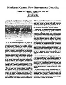
Routing in communication networks is based on shortest paths 关or the best approximation due to, e.g., the distracting influence of border gateway protocol 共BGP兲兴 between any two nodes of the network. The resources of a network are most efficiently used when traffic follows shortest paths 关1兴. In large complex networks, not all links have equal importance. For example, if two clusters are connected by one link, the removal of this link will disable all the traffic flowing between these two clusters. In contrast, the removal of a link connecting to a dead end whose degree is one, will have no effect on the other parts of the network. The importance of links is of primary interest for network resilience to attacks 关2,3兴 and immunization against epidemics 关4兴. A good measure for “link or node importance” is the betweenness Bl共Bn兲 of a link 共node兲, which is defined as the number of shortest paths between all possible pairs of nodes in the network that traverse the link 共node兲. The betweenness Bl共Bn兲 which incorporates global information is a simplified quantity to assess the maximum possible traffic. Assuming that a unit packet is transmitted between each node pair, the betweenness Bl is the total amount of packets passing through a link. The overlay G艛SPT, as shown in Fig. 1, is the union of the shortest paths between all possible node pairs, and it can be regarded as the “transport overlay network” on top of the underlying network topology or substrate. The overlay G艛SPT, which is a subgraph of the substrate in a weighted graph, determines the network’s performance: any link removed in G艛SPT will definitely impact at least those flows of traffic that pass over that link. Since all the traffic traverses only the overlay G艛SPT and all the nodes in the substrate also appear in the overlay G艛SPT, the betweenness of a node in the substrate is equal to the betweenness of that node in the overlay G艛SPT. A link in the substrate has betweenness 0 if it does not belong to the overlay G艛SPT. Otherwise, its link 1539-3755/2008/77共4兲/046105共10兲

betweenness is the same as that in the overlay G艛SPT. In this paper, we study the link betweenness of the overlay G艛SPT. The study of betweenness usually deals with scale-free trees 关5–8兴 or scale-free networks 关9,10兴 whose degree distribution follow a power law, i.e., Pr关D = k兴 ⬃ k−␥. However, the overlay G艛SPT that we are going to examine possesses different degree distribution, e.g., uniform, exponential or power law distribution. The structure of the overlay network G艛SPT can be controlled, e.g., by tuning the extreme value index ␣ of the independent and identically distributed 共IID兲 polynomial link weights 关11兴. In the strong disorder limit 共␣ → 0兲, the overlay G艛SPT共␣ → 0兲 becomes the minimum spanning tree 共MST兲, a tree which has the minimum total weight of all possible spanning trees. The betweenness of the MST for various network models and real-world complex networks are surprisingly found to follow a power law. This power law betweenness distribution for MST holds more generally than in Erdös-Rényi random graph and scale-free networks as found in Ref. 关12兴. In addition, the relationship between the structural characteristics and its betweenness distribution is investigated. We study the correlation between the link weights and the corresponding link betweenness when the system is in weak disorder, in-

046105-1

Overlay Network GUspt: union of shortest paths between all node pairs.

Link weight distribution e.g. Fw(x) = xα1x∈[0,1] +1x∈(1,∞) w

Underlying Topology G(N,L)

FIG. 1. 共Color online兲 The overlay network G艛SPT. ©2008 The American Physical Society


WANG, HERNANDEZ, AND VAN MIEGHEM

-5

10

-10

-10

10

10 10

-15

-15

10 α = 0.2

-20

0.30

E[w | Bl = j]

10

-5

-20

10

0.30 α = 1.0

0.25

0.20

0.15

0.15

0.10

0.10

0.05

0.05

0.00

1

10

100

0.25

0.20

w

E[w | Bl = j]

10

w 1000

1

link betweenness j

10

0.00 1000

100

link betweenness j

(a)

(b)

1.0 α = 2.0

0.6

0.6

0.4

0.4

0.2

E[w | Bl = j]

0.8

1.0 α = 4.0

0.8

0.8

0.6

0.6

0.4

0.4

w

E[w | Bl = j]

0.8

w

stead of the correlation between the node betweenness and the node degree as in Refs. 关12,13兴. In Sec. II, we explain the notions of structural changes in the overlay G艛SPT共␣兲 as we tune the extreme value index ␣. Simulation scenarios are mentioned. The correlation between link weight and its betweenness is investigated in Sec. III. Furthermore, the link betweenness distribution of the overlay G艛SPT that characterizes the traffic distribution is examined in Sec. IV. If ␣ → 0, the overlay G艛SPT becomes the MST. The link betweenness of such overlay trees on top of network models as well as real-world networks are compared together with other classes of trees in Sec. V. Finally, our results are summarized in Sec. VI.

0.2 0.2

0.0 1

II. BASIC NOTIONS AND SIMULATION SCENARIOS

2

4

6 8

10

2

Fw共x兲 = x␣1x僆关0,1兴 + 1x僆共1,⬁兲,

␣ ⬎ 0,

共1兲

where the indicator function 1x is one if x is true else it is zero. The corresponding density is f w共x兲 = ␣x␣−1 , 0 ⱕ x ⱕ 1. The exponent

␣ = lim x↓0

lnFw共x兲 lnx

is called the extreme value index of the probability distribution of w and ␣ = 1 for uniform distributions. The link weights in a network are IID according to Eq. 共1兲. In Ref. 关11兴, a transition is observed around a critical extreme value index ␣c 关15兴, that is defined by Pr关GU SPT共␣=␣c兲 = MST兴 = 21 : When ␣ → 0 共or in the ␣ ⬍ ␣c regime for large networks兲, all flows are transported over the MST. Hence, G艛SPT共␣→0兲 = MST is also called an overlay tree. When ␣ ⬎ ␣c, transport in the network traverses many links. The ␣ → 0 共or ␣ ⬍ ␣c for large networks兲 regime corresponds to the strong disorder limit, where the total weight of a path is characterized by the maximum link weight along the path. The shortest path in this case is the path with the minimum value of the maximum link weight. When all links contributes to the total weight of the shortest path, the system is weak disordered, e.g., ␣ ⬎ ␣c. In fact, other distributions that could lead to strong disorder 关16兴 would arrive at similar betweenness behavior, because the MST is probabilistically the same for various IID link weights distributions 关17兴. For the underlying topology, called the substrate, we consider the following complex network models: the ErdösRényi random graph G p共N兲, the square and the cubic lattice, and the Barabási-Albert 共BA兲 power law model 关18兴. Traditionally, complex networks have been modeled as ErdösRényi random graphs G p共N兲, which can be generated from a set of N nodes by randomly assigning a link with probability

6 8

link betweenness j (c)

We restrict ourselves to additive link weights and nondirected graphs. Hence, the shortest path between two nodes is the path that minimizes the sum of the weights along the path. Since the shortest path 共SP兲 is mainly sensitive to the smaller, non-negative link weights, the simplest distribution of the link weight w with a distinct different behavior for small values than a regular distribution 共Ref. 关14兴, Chap. 16兲 is the polynomial distribution

4

100

2

0.2

0.0 1

2

3

4 5 67

10

2

link betweenness j

3

4 5 67

100

(d)

FIG. 2. 共Color online兲 The link weight w 共cross兲 versus its link betweenness j and E关兩w兩Bl = j兴共square兲 the average link weight of links with given betweenness j in the overlay G艛SPT on top of Erdös-Rényi random graph G0.4共100兲.

p to each pair of nodes. In addition to their analytic tractability, the Erdös-Rényi random graphs are reasonably accurate models for peer-to-peer networks and ad hoc networks. The square lattice, in which each node has four neighbors, is the basic model of a transport network 共Manhattan grid兲 as well as in percolation theory 关19兴 and is frequently used to study the network traffic 关20兴. The power law degree distribution is followed by many natural and artificial networks such as the scientific collaborations 关21兴, the world-wide web, and the Internet 关22兴. We carried out 104 iterations for each simulation. Within each iteration, we randomly generate an underlying topology. Polynomial link weights with parameter ␣ are assigned independently to each link. The overlay G艛SPT as well as its betweenness is found by calculating the shortest paths between all node pairs with Dijkstra’s algorithm 关23兴 for weak disorder regime. For the strong disorder limit ␣ → 0, G艛SPT = MST is found by Kruskal’s algorithm 关24兴 on the corresponding network with uniform link weights, because with IID link weights, the structure of the MST is probabilistically the same for various link weights distributions 关17兴. III. LINK WEIGHT VERSUS LINK BETWEENNESS

Does a lower link weight implies a high link betweenness Bl? When polynomial link weights are independently assigned to links in the substrate, we randomly choose a link in each overlay network G艛SPT. The betweenness of this link and the corresponding link weight are plotted in Fig. 2. According to Ref. 关11兴, ␣c = 0.2 关15兴 for Erdös-Rényi random graph with N = 100 nodes. When the system is weakly disordered, i.e., ␣ ⬎ ␣c 关Figs. 2共b兲–2共d兲兴, a link with lower link weight is more likely to have higher betweenness. However, when ␣ = 0.2 关Fig. 2共a兲兴, where link weights possess relatively strong fluctuations, the correlation between link weight and betweenness disappears. Hence, a negative correlation exists between the link weight and its betweenness

046105-2


BETWEENNESS CENTRALITY IN A WEIGHTED NETWORK

TABLE I. The correlation coefficient between weight and betweenness of a link.

␣ G艛SPT G艛SPT G艛SPT G艛SPT

on on on on

G0.4共100兲 square lattice N = 100 cubic lattice N = 125 BA N = 100, m = 3

0.2

1.0

2.0

4.0

8.0

16.0

−0.06 −0.22 −0.18 −0.12

−0.61 −0.53 −0.60 −0.53

−0.70 −0.54 −0.66 −0.66

−0.78 −0.53 −0.67 −0.60

−0.84 −0.53 −0.68 −0.50

−0.84 −0.53 −0.68 −0.49

for the weak disorder regime. The correlation becomes stronger as ␣ increases, as illustrated in Table I where the linear correlation coefficient is equal to the covariance between the two random variables divided by the product of their standard deviations. The increasing strength of the correlation for larger ␣ is also reflected by Fig. 2, where as ␣ increases, the plot of link weights become narrower. The correlation between the weight and the betweenness of the link is shown to be dependent on the underlying graph as well as on the extreme value index ␣ of the polynomial link weight distribution. For homogeneous network such as the Erdös-Rényi random graph and lattice, the correlation coefficient increases monotonically as ␣ increases. However, in a the nonhomogeneous topology such as the BA power law substrate, the correlation coefficient decreases after a maximum has been reached. In a homogeneous network, when ␣ is large, a link with lower link weight tends to attract more traffic. While in a nonhomogeneous topology, the relative importance of a link or its connectivity in substrate is also an determinant factor for its betweenness. In short, both the nonhomogeneity of the underlying topology and the link weight disorder 共e.g., a smaller ␣兲 contribute to the nonhomogeneity of the overlay G艛SPT, which reduces the correlation between link weight and betweenness. IV. LINK BETWEENNESS DISTRIBUTION OF OVERLAY G SPT

The link betweenness represents the total traffic passing through a link if a unit packet is transmitted between each node pair. Hence, the link betweenness distribution reflects how the traffic is distributed over the network. A. Overlay G SPT on top of complex network models

As shown in Fig. 3共a兲, the traffic on the overlay G艛SPT on α = 1.0 α = 2.0 α = 4.0

-1

Pr[Bl = j]

Pr[Bl = j]

10

10

-1

10

-2

10

10

-2

10

-3

10

-3

10

-4

10

-4

1

10

100

link betweenness j (a)

1000

α = 0.2 α = 0.02

top of G0.4共100兲 varies less for large ␣, because the betweenness is distributed within a small range. When ␣ is small, as shown in Fig. 3共b兲, the betweenness is ranging between approximately 1 − 2500 for N = 100 and peaks appear on the betweenness at n共N − n兲, where 1 ⱕ n ⱕ N − 1. A link is called critical if its removal will disconnect the overlay G艛SPT into two clusters with n and N − n nodes. The betweenness of such critical link is n共N − n兲, because all the traffic with source and destination separated in these two clusters will traverse this link. However, if a link has betweenness n共N − n兲, the removal of this link does not necessarily disconnect the overlay graph. As we decrease the extreme value index ␣, the overlay G艛SPT contains less links and it becomes tree-like or even an exact tree. Any link in a tree is critical. We consider, for example, the Erdös-Rényi random graph G0.4共100兲. When ␣ = 0.2, the average number of links in the overlay is 107.2. Within such a sparse overlay topology, a link is very likely to be critical, which contributes to the peaks in Fig. 3共b兲. A sparse overlay G艛SPT is composed of the minimum spanning tree and few shortcuts, that direct a small part of the traffic. The largest link betweenness 2500 comes from the critical link which could separate the overlay network into two clusters each with N2 = 50 nodes. A link has higher betweenness if it is critical and the maximal link betweenness is achieved when n = 关 N2 兴. Hence, the betweenness of any link in a graph with N nodes obeys Bl ⱕ

N N N− . 2 2

2.85 -1.6

*j

10

100

link betweenness j

1000

(b)

FIG. 3. 共Color online兲 The probability density function 共PDF兲 of link betweenness Bl in the overlay G艛SPT on top of G0.4共100兲. The PDF for ␣ = 0.02 is linear fitted by the dashed line.

共2兲

When the overlay becomes a tree, the magnitude of peaks at n共N − n兲 also depends on the structure of the tree. For example, if the overlay network is a star with N nodes, the link betweenness is always N − 1. And if G艛SPT is a line graph, the betweenness of a link is n共N − n兲 with n uniformly distributed over 关1 , N − 1兴. We find that the betweenness distribution of the overlay tree G艛SPT共␣→0兲 on top of the ErdösRényi random graph G p共N兲 follows a power law Pr关Bl = j兴 = c0 j−c,

1

冉冊

N−1ⱕjⱕ

冉冊 N N N− 2 2

共3兲

with exponent c = 1.6. Further, we observe that the overlay tree G艛SPT共␣→0兲 on top of other complex network models such as the lattice, cubic lattice or a BA model also seems to possess a power law betweenness distribution as illustrated in Fig. 4. The lower bound N − 1 of the betweenness in a tree is attained at a link connected to a degree 1 node while the upper bound obeys Eq. 共2兲. The exponent c we found for

046105-3



-1

-2 -4

Pr[Bl = j]

uspt

10

j−1.5*102.7 G on top of square lattice, N = 100 uspt −1.33

j G

uspt −1.6

Pr[Bl = j]

j

2.2

*10

-6

10

-8

10

-10

10

*10 on top of G (100)

10

-7

10

-9

10

-11

10

2.8

-5

10

-12

0.8

high energy collaborations

-3

10

10

3.1

j *10 G on top of cubic lattice, N = 125

−1

10

AS Internet topology

10

on top of BA model, N = 100, m = 3

uspt −1.7

Pr[Bl = j]

G

-13

-14

10

10

10

11

10

12

10

10

13

14

10

15

10

betweenness j

10

16

9

17

10

10

10

10

10

11

12

10

10

13

14

10

15

10

betweenness j

10

-1

Gnutella (Crawl2)

Pr[Bl = j]

10

-6

10

-8

10

-6

9

Erdös-Rényi 共c = 1.6兲 lattice 共c = 1.33兲 and BA model 共c = 1.7兲 with N ⬃ 100 are the same as observed in Ref. 关25兴 with N ⬃ 8100. The scaling exponent c seems insensitive to the size N of the network. Additional simulations for ErdösRényi random graph suggest that the exponent c is independent of the size N of the underlying graph as well as the link density p, if p is larger than the disconnectivity threshold pc ⬃ ln N / N. For example, the power exponent c = 1.6 remains the same for the substrate G0.4共100兲 , G0.4共50兲 , G0.8共100兲 and the Erdös-Rényi random graph in 关12兴 with N = 104 nodes and L = 2N links. B. Overlay tree G SPT(␣\0) on top of real networks

As found in Sec. IV A and Fig. 4, an overlay tree G艛SPT共␣→0兲 follow a power law betweenness distribution when the substrate is an Erdös-Rényi random graph, a square or cubic lattice or a BA power law graph. It would be especially interesting to examine whether the power law link betweenness distribution still holds for overlay trees G艛SPT共␣→0兲 on top of real-world networks. Hence, we perform a statistical analysis of real data sets, representing the topology of different real-world networks. On top of each, usually large network, 100 realizations of IID uniform link weights assignments are carried out. Within each realization, the MST, equivalent to the overlay tree G艛SPT共␣→0兲, is found with the Kruskal algorithm 关24兴. The complex networks come from a wide range of systems in nature and society: The Internet network at the level of autonomous systems 关26兴; the Gnutella 关27兴 snapshots 共Crawl2兲 retrieved from firewire.com; the air transportation network representing the world wide airport connections, documented at the Bureau of Transportation Statistics 共http://www.bts.gov兲 database; the Western States Power Grid of the United States 关28兴; the coauthorship network 关29兴 between scientists posting preprints on the High-Energy Theory E-Print Archive between Jan 1, 1995 and December 31, 1999; two citation networks 关30兴 created using the Web of Science database 共Kohonen and SciMet兲; the coauthorship network 关31兴 of scientists

11

10

12

10

13

10

betweenness j

5

10

6

10

7

10

betweenness j

8

10

10

FIG. 5. 共Color online兲 Betweenness distribution 共+兲 of G艛SPT共␣→0兲 on top of real network topologies. The line is the linear curve fitting.

working on network theory and experiment; the network representing soccer players association to Dutch soccer teams 关32兴; the network of American football games between division IA colleges during regular season Fall 2000 关33兴; and the adjacency network 关34兴 of common adjectives and nouns in the novel David Copperfield by Charles Dickens. As shown in Fig. 5 as well as Figs. 6 and 7, the betweenness distribution of these overlay trees on top of real networks follows, surprisingly, for almost all a power law, while their corresponding degree distribution of the tree 共see Figs. 8–10兲 may differ significantly. The power law betweenness distribution of the overlay tree G艛SPT共␣→0兲 or MST implies that a set of links in the MST possess a much higher betweenness. In Ref. 关25兴, it is found that the infinite incipient percolation cluster 共IIC兲, a subgraph of the MST has a significantly higher average betweenness than the entire MST, and the betweenness distribution of the IIC also satisfies a power law. But why does the betweenness distribution of a MST follow a power law? Is that due to the network topology, a particular link weight -1

-1

10

10

power grid

-3

10

Dutch soccer

-3

10

-5

Pr[Bl = j]

FIG. 4. 共Color online兲 Link betweenness distribution 共markers兲 of overlay tree G艛SPT共␣→0兲 on top of complex network models and the corresponding linear fitting 共dashed lines兲.

10

10

10

-7

10

-9

10

-5

10

-7

10

-11

10

-9

10

-13

10

9

10

10

11

10

12

10

13

10

14

10

15

10

7

10

8

10

9

10

-2

11

10

10

betweenness j -2

web of science citations (Kohonen)

10

10

10

betweenness j 10

-4

web of science citations (SciMet)

-4

10

Pr[Bl = j]

10

Pr[Bl = j]

Betweenness j

Pr[Bl = j]

10

8

10

3

-4

10

10

-12

2

10

-5

10

−3

-3

10

-10

10

10

American football

-2

10

-4

Pr[Bl = j]

10

10

-2

10

−2

-6

10

-8

10

-10

10

-6

10

-8

10

-10

10

10

-12

-12

10

10 9

10

10

10

11

10

12

10

betweenness j

13

10

14

10

15

10

8

10

9

10

10

10

11

10

12

10

13

10

14

10

betweenness j


046105-4


BETWEENNESS CENTRALITY IN A WEIGHTED NETWORK -1

science coauthorship network

-1

10

10

-6

10

-8

10

-3

10

Pr[D = j]

Pr[Bl = j]

-4

-4

10

-5

10

-10

-7

6

7

8

10

9

10

5

10

6

10

-2

7

10

10

2

betweenness j

-3

10

4

6

8

10

12

14

16

2

Degree j

Pr[D = j]

10

-6

10

-8

10

-2

10

-3

10

-4

8

9

10

10

10

10

11

12

10

10

13

10

10

12

14

16

webofsciencecitations(SciMet)

-2

10

-3

10

-4 -5

10

14

2

1

betweenness j

10

10

10

-12

8

-1

-5

10

6

10

10

-10

10

4

Degree j

web of science citations (Kohonen)

-1

10

air transportation

-4

Pr[Bl = j]

10

-4

8

10

Dutch soccer

-2

10

-5

betweenness j 10

-3

10

10

10

10

10

-4

10 10

-1

10

10

-6

10

10

power grid

-2

Pr[D = j]

Pr[Bl = j]

word adjacencies

-2

10

Pr[D = j]

10

-2

10

3 4 5 67

2

10

3 4 5 67

Degree j

100

2

2

1

3

4

5 6 7 89

Degreej

2

10

3


FIG. 9. 共Color online兲 Degree distribution of G艛SPT共␣⬍␣c兲 on top of real network topologies.

distribution function or the fact that link weights are independently and identically distributed? The betweenness of the overlay tree follows a power law distribution no matter the substrate is a traditional complex network model or a real network, provided the substrate is denser than a tree. When the substrate is close to a tree, the overlay tree is almost the same as the substrate and the corresponding betweenness distribution does not necessarily follow a power law. Hence, the power law betweenness distribution does not hold for any tree structure but seems to hold for the overlay tree G艛SPT共␣→0兲 on top of a substrate which is not too sparse. With IID link weights, the structure of the overlay tree or MST is probabilistically the same for various link weight distributions, because the ranking of the link weights suffices to construct the MST. Therefore, the IID link weights compared to the network topology and link weight distribution, contribute more to the power law betweenness distribution of the MST for various networks. In fact, with IID link weights, the equivalent Kruskal growth process of the MST starts from N individual nodes and in each step an arbitrary link in the substrate is added while links generating loops are forbidden. However, the power exponent c of the betweenness

distribution of a MST is determined by the network topology, due to the exclusion of links that generating loops in the growth process of the MST. The relationship between the topological characteristics of a network and the exponent c of the betweenness distribution of the corresponding MST is studied in Sec. V B.

V. BETWEENNESS DISTRIBUTION OF TREES

Since the path between each node pair is unique in a tree and is independent of link weights, the betweenness of a tree depends purely on its tree structure. In the strong disorder limit 共␣ → 0兲, the betweenness distribution depends on the structure of G艛SPT共␣→0兲 or MST. In this way, we are able to compare the tree structure of overlay G艛SPT共␣→0兲 to other classes of trees via the link betweenness distribution. Although trees are special graphs, real-world networks such as the autonomous systems in the Internet 关35兴 can be modeled by trees or treelike graphs with a negligible number of shortcuts. science coauthorship network

-1

10

Pr[D = j]

Pr[D = j]

-2

10

-3

10

-4

10

-5

10

5

10

15

20

25

10

-1

10

-2

10

-3

10

-4

10

-5

10

-6

AS Internet topology

-2

10

-3

10

-3

10 -4

-4

10 2 1

10

100

4

6

8

12

10

-3

10

-4

10

-5

Pr[D = j]

-2

0.2

16

18

2

4

6

8

10

12

14

16

18

degree j air transportation

10

American football

0.3

Pr[D = j]

Pr[D = j]

10

Gnutella (Crawl2)

14

Degree j

1000

Degree j

10

-1

-1

-2

10

10

Degree j 10

word adjacencies

-1

10

Pr[D = j]

high energy collaborations

10

Pr[D = j]

-1

-2

10

-3

10

-4

10

0.1

-5

1

2

3

4 5 6

10

2

Degree j

3

4 5 6

10

0.0 100

1

2

3

4

Degree j

5

6

7

FIG. 8. 共Color online兲 Degree distribution of G艛SPT共␣→0兲 on top of real network topologies.

1

2

3

4

5 6 789

10

2

3

4 5

Degree j

FIG. 10. 共Color online兲 Degree distribution of G艛SPT共␣→0兲 on top of real network topologies.

046105-5



In this section we compare the following trees. 共a兲 Three tree models: the k-ary tree, the scale-free trees, and the uniform recursive tree URT. 共b兲 The overlay tree G艛SPT共␣→0兲 on top of complex network models: the Erdös-Rényi random graph, the square or cubic lattice, and the BA power law model. 共c兲 The overlay tree G艛SPT共␣→0兲 on top of real complex networks. The class 共b兲 and 共c兲 have been shown to possess power law betweenness distribution. Hence, it is interesting to first examine whether the class 共a兲 has such power law betweenness distribution. A link l in any tree connects two clusters with size 1 ⱕ 兩Cl兩 ⱕ N2 and N − 兩Cl兩. The betweenness of a link l is Bl = 兩Cl兩共N − 兩Cl兩兲, because traffic traverses the link l if and only if the source and destination lie in the two clusters separated by l. If 兩Cl兩 = o共N兲, which holds for all but a few large clusters, then we have Bl ⬃ 兩Cl兩 · N for large N.

1. k-ary tree

We investigate the k-ary tree 关14兴 of depth 关36兴 D, where each node has exactly k children. In a k-ary tree the total number of nodes is

冦

冧

kj . N共D兲 − 1

is given in Appendix B. 2. Scale-free trees

A scale-free tree contains initially only one node, the root. Then, at each step a new node is attached to one of the existing node. The probability that a new node connects to a certain existing node is proportional to the attractiveness of the old node, defined as A共v兲 = a + q,

Pr关Din = q兴 = 共q + a兲−共2+a兲 . Early in 2002, the power law betweenness distribution with c = 2 for the scale-free trees is solved analytically by Goh et al. 关38兴. Here, we relate the betweenness distribution to the subtree size distribution, which is derived by Fekete and Vattay 关5兴. In our notation, the probability distribution of the size of a subtree rooted at a random node in a scale-free tree with N nodes is Pr关兩T共N兲兩 = k兴 =

⬇共1 − ␤兲

kD+1 , 共N共D兲 − 1兲共kn − n + 1兲

1 , k2

Pr关Bl = kN兴 ⬇ 共1 − ␤兲

n = N共D − j兲 and 1 ⱕ j ⱕ D. The approximate betweenness distribution Pr关Bl ⬃ n · N兴 =

1−␤ N−␤ , N − 1 共k − ␤兲共k + 1 − ␤兲

共5兲

共6兲

1 僆关0 , 1兴. When ␤ = 21 , the scale-free tree is exwhere ␤ = 1+a actly the BA tree, with m = 1 in the BA model. When ␤ = 0, the tree becomes a uniform recursive tree URT. Hence, the probability that a link has load approximately kN will be

Hence, Pr关兩Cl兩 = n兴 =

1ⱕjⱕD 共4兲

A link is called the jth level link if it connects two nodes which is j and j − 1 hops away from the root. The removal of a jth level link disconnect the graph into two clusters: one is a k-ary tree of depth D − j with N共D − j兲 nodes and the other cluster has N共D兲 − N共D − j兲 nodes. Since there are k j jth 共1 ⱕ j ⱕ D兲 level links Pr关兩Cl兩 = N共D − j兲兴 =

kj , N共D兲 − 1

where a ⬎ 0 denotes the initial attractiveness and q is the in-degree of node v, the number of links connected to the node. The corresponding in-degree distribution 关37兴 is

A. Betweenness distribution of tree models

kD+1 − 1 , k ⫽ 1, k−1 N共D兲 = 1 + k + k2 + ¯ + kD = 1 + D, k = 1.

Pr兵Bl = N共D − j兲关N共D兲 − N共D − j兲兴其 =

kD+1 , 关N共D兲 − 1兴共kn − n + 1兲

n = N共D − j兲 and 1 ⱕ j ⱕ D follows an inverse power law with exponent c = 1. Two exceptions are the line graph, where k = 1 , Pr关Bl = n共N − n兲兴 1 = N−1 , 1 ⱕ n ⱕ N − 1 and the star where k = N − 1 , Pr关Bl = N − 1兴 = 1. A rigorous analysis based on

1 . k2

The inverse square power law betweenness distribution with c = 2 holds for the class of scale-free trees where the scaling property of the degree can be finely tuned by the initial attractiveness a. Further as shown in Ref. 关6兴, if N Bl 共 N2 兲2, its complementary distribution can be approximated by the 1 power law Pr关Bl ⱖ x兴 = 共1 − ␣兲N Bl which leads to our c = 2 scaling for the probability distribution of Bl. The link and node betweenness distribution is considered to be same in a tree 关39兴. Szabó et al. 关7兴 found the scaling exponent c = 2 for node betweenness in a BA tree with a “mean-field” approximation. The rigorous proof of the heuristic result of 关7兴 has been provided by Bollobás and Ridordan in Ref. 关8兴.

046105-6



TABLE II. Topological characteristics of tree models and overlay tree on top of network models.

the corresponding tree structure which can be partially characterized by the average hop count E关H兴共or the average number of links兲 of the shortest path and the standard deviation sdev关D兴 of the degree, because the average degree in any tree is E关D兴 = 2共N − 1兲 / N = 2 − N2 . We compare class 共a兲 and 共b兲 in Table II and class 共c兲 in Table III. With a similar number of nodes in Table II we find the following. The scaling exponent c seems to be negatively correlated with the E关H兴 except for the k-ary tree. The scaling exponent c seems to be positively correlated with the sdev关D兴 standard deviation of the degree except for the k-ary tree. The higher the variance of the degree is, the more traffic among links varies. The scaling exponent c seems to be insensitive to the size N of the tree. A same slope c is obtained for different substrate size, e.g., the k-ary tree, and the G艛SPT共␣→0兲 on top of network models as mentioned in Sec. IV A. However, the E关H兴 behaves as a function of N and the sdev关D兴 can slightly depend on N with the fixed average E关D兴 ⬇ 2. Hence, the correlation between c and E关H兴 as well as sdev关D兴 may become weaker or even disappear when networks with different sizes are considered, which will be further examined for real-world networks in Table III. The URT and the class of scale-free trees 共e.g., the BA tree兲 discussed in Sec. V A 2, have c → 2.0 for large N and N Bl 共 N2 兲2. Compared to URT, the degree of the BA tree varies more and has higher scaling exponent c 共see Table II兲, when the complete range Bl 僆共N − 1 , N2 共N − N2 兲兴 is taken into account. The scaling exponent c of betweenness distribution varies from c = 1 for the k-ary tree to c = 2 for scale-free trees. For overlay trees on top of real networks G共N , L兲 with N nodes and L links in Table III. The exponent c ranges from 1.5 to 1.9, while the network size varies from N = 112 to N = 12254. The scaling exponent c does not seem to be dependent on the size N of the topology. The negative correlation between hop count E关H兴 and c disappear because E关H兴 is positively correlated with N. The positive correlation between sdev关D兴 and c still holds for most of the considered networks. The overlay trees possess different degree distributions as plotted in Figs. 6–10. The overlay tree of networks that are marked with a star in Table III possesses a

N BA tree URT G艛SPT共␣⬍␣c兲 on BA model 共m = 3兲 G艛SPT共␣⬍␣c兲 on G0.8共100兲 G艛SPT共␣⬍␣c兲 on cubic lattice G艛SPT共␣⬍␣c兲 on square lattice G艛SPT共␣⬍␣c兲 on square lattice k-ary tree 关40兴

100 100 100 100 125 100 144 100

c

E关H兴

2.3 4.7 2.1 6.6 1.7 9.6 1.6 9.8 1.5 12.8 1.3 13.4 1.3 16.8 1 E关H共k兲兴

sdev关D兴 2.38 1.36 1.04 1.04 0.92 0.81 0.82 冑k − 1

An URT 共␤ = 0兲 possesses in fact exponential degree distribution. A rigorous derivation of link betweenness distribution for URT is given in Appendix A.

B. Comparison of betweenness distribution of overlay trees and tree models

All the three classes of trees have been shown to follow approximately a power law betweenness distributions. The power law betweenness distribution has been proved for class 共a兲 tree models in Sec. V A, while for class 共b兲 overlay tree on top of network models and 共c兲 overlay tree on top of real networks it seems to arise from the random sampling of the overlay tree 共caused by the IID link weights兲 as explained in Sec. IV B. The slope of the betweenness distribution in log-log scale or, equivalently, the power exponent c of the corresponding power law distribution 共3兲, characterizes the variance of the traffic carried along links in the network. High values of c can be interpreted as a high concentration of traffic on the most important links. The betweenness distribution of a tree depends purely on the structure of the tree. Hence, we further examine the relationship between the scaling exponent c and

TABLE III. Topological characteristics of overlay tree on top of real-world networks. The overlay tree of networks that are marked with a star possesses a power law degree distribution.

Internet As topology* Web of Science citations 共koh兲* Gnutella Crawl2* Science coauthorship network Word adjacencies Air Transportation* Web of Science citations共scimet兲* High Energy collaborations Dutch soccer Power grid American football

N

L

c

E关H兴

sdev关D兴

12254 3704 1568 379 112 2179 2678 5835 685 4941 115

25319 12673 1906 914 850 31326 10385 13815 10310 6594 613

1.9 1.9 1.9 1.8 1.8 1.7 1.7 1.7 1.7 1.6 1.5

12.2 14.6 11.6 14.1 7.7 17.9 22.18 31.1 22.7 58.9 11.8

16 6.0 4.3 1.6 1.6 2.8 1.9 1.5 1.4 1.2 1.0

046105-7



10

6 5

E[H]

sdev[D]

10

4 3

9 8 7 6 5

2

4

1

3

1.4

1.6

1.8

power exponent c

2.0

2.2

1.4

1.6

1.8

power exponent c

2.0

2.2

FIG. 11. 共Color online兲 Relationship between the power exponent c of the betweenness and the standard deviation sdev关D兴 and the average hop count E关H兴 of the tree.

points downhill 关41兴, a signature of the intrinsic fractal properties of webs. And recently, Kitsak et al. 关9兴 have brought fractal properties of networks into the betweenness analysis. In the weak disorder regime, traffic flows over more links than that of the MST. The negative correlation between link weight and betweenness also depends on ␣, the strength of link weight disorder and the structure of the underlying topology. Both a stronger disorder in link weights and the nonhomogeneity of the substrate reduce the correlation.

ACKNOWLEDGMENTS

power law degree distribution. Hence, the betweenness distribution of scale-free networks does not necessarily follow the same power law exponent c, while a similar exponent c can be obtained in networks with different degree distributions. The relationship between the sdev关D兴 as well as the E关H兴 and the scaling exponent c of betweenness distribution is given in Fig. 11. Points lying on the line are for networks listed in Table II with similar topology size N. The approximately positive correlation between sdev关D兴 and c can be observed for all the three classes. Since the average degree E关D兴 = 2共N − 1兲 / N ⬇ 2 in a tree is almost constant, a higher degree variance implies more nodes with higher degree or/ and more nodes with degree 1. The betweenness of links connected to a degree 1 node is always the minimum N − 1 while the traffic passing through a high degree node is split by links connected to this node. Both contribute to a higher scaling exponent c.

VI. CONCLUSION

In this paper, we examine the traffic in a weighted network via the link betweenness distribution of the corresponding transport overlay network G艛SPT共␣兲, the union of all shortest paths. In the strong disorder regime, all transport flows over the overlay tree G艛SPT共␣→0兲 = MST. Important new findings are the power law betweenness distribution specified in Eq. 共3兲 of trees: tree models such as scale-free trees and k-ary trees; overlay trees on top of traditional network models; overlay trees on top of real-world complex networks. The scaling exponent 1 ⬍ c ⱕ 2 for large networks is shown to be positively correlated with the sdev关D兴 of the corresponding tree and is insensitive to the network size N. Equipped with IID link weights, the overlay tree is, in fact, a random minimum spanning tree 共RMST兲. We conjecture that the scaling exponent c may be used to characterize these tree structures and probably the underlying topology. First, recall that any link in a tree connects two clusters with size 1 ⱕ 兩Cl兩 ⱕ N2 and N − 兩Cl兩 and Bl ⬃ 兩Cl兩 · N in Sec. V. The power law betweenness distribution implies approximately a same power law scaling for Pr关兩Cl兩 = n兴 ⬃ n−c the probability distribution of cluster size. Second, for the Internet As topology, our power law scaling of betweenness with c = 1.9 is the same as Pr关S = n兴 ⬃ n−1.9⫾0.1 the probability of finding n

This research was supported by the Netherlands Organization for Scientific Research 共NWO兲 under Project No. 643.000.503.

APPENDIX A: LINK BETWEENNESS DISTRIBUTION OF URT

A URT 关14兴 of size N is a random tree rooted at some node A. At each stage a node is attached uniformly to one of the existing nodes until the total number of nodes is equal to N. When the jth node is attached, the corresponding jth attached link is also added except that no link is added when we start from the root or the first node. In a tree, the traffic traverses the link if and only if the source and destination lies in different clusters separated by this link. In a URT, we define 兩T共N兲 j 兩 as the size of the subtree rooted at the jth attached node. The removal of the jth 共2 ⱕ j ⱕ N兲 attached link will separate the graph into two clusters with size 兩T共N兲 j 兩 and 兩. Correspondingly, the betweenness of the jth 共2 N − 兩T共N兲 j 共N兲兩 · 共N − 兩T 兩兲. The probability ⱕ j ⱕ N兲 attached link is 兩T共N兲 j j distribution of the size of the subtree 关42兴 equals

Pr关兩T共N兲 j 兩

共j − 1兲共N − j兲 ! 共N − k − 1兲! = k兴 = = 共N − 1兲 ! 共N − j − k + 1兲!

冉

N−k−1 j−2 N−1

冉冊

冊

j−1

共A1兲 Using the law of total probability 关14兴, we have for the URT that

046105-8

N

Pr关Bl = k共N − k兲兴 = 兺 Pr关Bl = k共N − k兲兩l = j兩兴Pr关l = j兴, j=2

1ⱕkⱕ

N . 2



A random link l is the jth attached link or attaches the jth 1 node to the URT with probability Pr关l = j兴 = N−1 . N N For k 僆关1 , 2 兴 and k ⫽ 2 , the conditional probability is

=

共N兲 Pr关Bl = k共N − k兲兩l = j兩兴 = Pr关兩T共N兲 j 兩 = k兴 + Pr关兩T j 兩 = N − k兴

Similarly,

because only if the size of the subtree rooted at node j is of 共N兲 size 兩T共N兲 j 兩 = k or of size 兩T j 兩 = N − k, the betweenness of the link l = j equals k共N − k兲. Combining both yields

N

兺 j=2

N

1 共N兲 Pr关Bl = k共N − k兲兴 = 兺 Pr关兩T共N兲 j 兩 = k兴 + Pr关兩T j 兩 = N − k兴. N − 1 j=2

共j − 1兲共N − j兲! = 共N − 1 − k兲 ! 共k + 1 − j兲! = 共N − 1 − k兲 !

Substituting Eq. 共A1兲 gives N

= 共N − 1 − k兲 !

共j − 1兲共N − j兲! 共N − k − 1兲! Pr关Bl = k共N − k兲兴 = 兺共N − 1兲共N − 1兲! j=2 共N − j − k + 1兲!

=

N

+

共j − 1兲共N − j兲! 共k − 1兲! . 兺共N − 1兲共N − 1兲! j=2 共k + 1 − j兲!

We use the identity m

j 兺 j=n

冉冊冉冉 a−j

b−j

=n

−

a+1−n b−n

冊冉冊 +

a+1−n b−1−n

兺 j=2

−m

a−m b−1−m

a+1−m

共j − 1兲共N − j兲! = 共k − 1兲 ! 共N − j − k + 1兲! − 1兲 !

冋冉

= 共k − 1兲 !

j 兺 j=1

冉

N−1−j N−k−j

N−1 N−k−1

冉

冊

Pr关Bl = k共N − k兲兴 = +

N−1

冊冉冊 +

冊

= 共k N−1

N−k−2

冊册

N N−k−1

Pr关Bl = k共N − k兲兴 =

冦

j 兺 j=1

冉

N−1−j k−j

冊

冋冉冊冉冊册 N−1 k−1

N−1

+

k−2

冉冊 N k−1

共N − 1 − k兲 ! N! . 共k − 1兲 ! 共N − k + 1兲!

共k − 1兲 ! N! 共N − k − 1兲! 共N − 1兲共N − 1兲! 共k + 1兲 ! 共N − k − 1兲!

共N − 1 − k兲 ! N! 共k − 1兲! 共N − 1兲共N − 1兲! 共k − 1兲 ! 共N − k + 1兲!

冉

=

1 1 N + 共N − 1兲共k + 1兲k 共N − k + 1兲共N − k兲

=

N−k k N + . 共N − 1兲k共N − k兲 k + 1 N − k + 1

冉

冊

冊

While for k = N2 = N2 , the probability has to be halved,

Pr关Bl = k共N − k兲兴 = Hence,

N−1

Hence,

共A2兲

b−1−m

and obtain N

冊冉

共k − 1兲 ! N! . 共k + 1兲 ! 共N − k − 1兲!

冉

N . 共N − 1兲k共k + 1兲

冊

冋册

N−k N N k + , k 僆 1, 2 共N − 1兲k共N − k兲 k + 1 N − k + 1

N N N if k = = . 共N − 1兲k共k + 1兲 2 2

APPENDIX B: LINK BETWEENNESS DISTRIBUTION OF A k-ARY TREE

and k ⫽

N , 2

冧

points 共x1 , y 1兲 and 共x2 , y 2兲 on this curve, we have D

If the link betweenness distribution 共4兲 of a k-ary tree follows a power law of the form y = c0xc, then for any two

共A3兲

y1 x1 c y 2 = 共 x2 兲 .

k Two nodes are selected: 关N共D兲 − 1 , N共D兲−1 兴 corresponding to j = D in Eq. 共4兲 and a random node 兵N共D − j兲关N共D兲 − N共D kj − j兲兴 , N共D兲−1 其.

046105-9



N共D − j兲关N共D兲 − N共D − j兲兴共kD−j+1 − 1兲共kD+1 − kD−j+1兲 = N共D兲 − 1 共kD+1 − 1 − k + 1兲共k − 1兲 =

共kD−j+1 − 1兲共kD+1 − kD−j+1兲 k共kD − 1兲共k − 1兲

=

kD共kD−j+1 − 1兲共1 − k−j兲 . 共kD − 1兲共k − 1兲

Hence, the link betweenness distribution of a k-ary tree is not a precise power distribution, but it is close to a power law with exponent c = −1, especially for larger k and D. The first and last point of link betweenness corresponds to j = 1 and j = N. Since N共D − 1兲关N共D兲 − N共D − 1兲兴 N共D兲 − 1

For large networks with large k and D, N共D − j兲关N共D兲 − N共D − j兲兴共kD−j+1 − 1兲共1 − k−j兲 ⯝ N共D兲 − 1 共k − 1兲 =

=

kD−j共k − k−共j−1兲 − k−共j−D兲 + k−D兲共k − 1兲

⯝k

D−j

=

冉冊 kj N共D兲−1 kD N共D兲−1

−1

冏

kD共kD−j+1 − 1兲共1 − k−j兲共kD − 1兲共k − 1兲

= kD−1 =

冉

兩

兩

kj N共D兲−1 j=1 kD N共D兲−1

冊

冏

j=1

−1

.

The first and the last points always lie on a power law curve with exponent c = −1. Hence, an exceptional case is for D = 2, which is an exact power law although D is small.

.

关1兴 P. Van Mieghem, Data Communications Networking 共Techne Press, Amsterdam, 2006兲. 关2兴 R. Albert, H. Jeong, and A.-L. Barabàsi, Nature 共London兲 406, 378 共2000兲. 关3兴 R. Cohen, K. Erez, D. ben-Avraham, and S. Havlin, Phys. Rev. Lett. 86, 3682 共2001兲. 关4兴 R. Pastor-Satorras and A. Vespignani, Phys. Rev. Lett. 86, 3200 共2001兲. 关5兴 A. Fekete, G. Vattay, and L. Kocarev, Phys. Rev. E 73, 046102 共2006兲. 关6兴 A. Fekete, G. Vattay, and L. Kocarev, Complexus 3, 97 共2006兲. 关7兴 G. Szabó, M. Alava, and J. Kertész, Phys. Rev. E 66, 026101 共2002兲. 关8兴 B. Bollobás and O. Riordan, Phys. Rev. E 69, 036114 共2004兲. 关9兴 M. Kitsak, S. Havlin, G. Paul, M. Riccaboni, F. Pammolli, and H. E. Stanley, Phys. Rev. E 75, 056115 共2007兲. 关10兴 K.-I. Goh, B. Kahng, and D. Kim, Phys. Rev. Lett. 87, 278701 共2001兲. 关11兴 P. Van Mieghem and S. M. Magdalena, Phys. Rev. E 72, 056138 共2005兲. 关12兴 K.-I. Goh, J. D. Noh, B. Kahng, and D. Kim, Phys. Rev. E 72, 017102 共2005兲. 关13兴 M. Barthélemy, Eur. Phys. J. B 38, 163 共2004兲. 关14兴 P. Van Mieghem, Performance Analysis of Communications Systems and Networks 共Cambridge University Press, Cambridge, 2006兲. 关15兴 ␣c depends on the network topology as well as the size N of the network. 关16兴 Y. Chen, E. Lopez, S. Havlin, and H. E. Stanley, Phys. Rev. Lett. 96, 068702 共2006兲. 关17兴 P. Van Mieghem and S. van Langen, Phys. Rev. E 71, 056113 共2005兲. 关18兴 A.-L. Barabási and R. Albert, Science 286, 509 共1999兲. 关19兴 R. T. Smythe and C. John, Wierman. First-Passage Percolation on the Square Lattice 共Springer, Berlin, 1978兲. 关20兴 T. Ohira and R. Sawatari, Phys. Rev. E 58, 193 共1998兲. 关21兴 M. E. J. Newman, Phys. Rev. E 64, 016131 共2001兲. 关22兴 M. Faloutsos, P. Faloutsos, and C. Faloutsos, ACM Comput.

Commun. Rev. 29, 251 共1999兲. 关23兴 E. W. Dijkstra, Numer. Math. 1, 269 共1959兲. 关24兴 T. H. Cormen, C. E. Leiserson, and R. L. Rivest, An Introduction to Algorithms 共MIT Press, Boston, 1991兲. 关25兴 Z. Wu, L. A. Braunstein, S. Havlin, and H. E. Stanley, Phys. Rev. Lett. 96, 148702 共2006兲. 关26兴 R. Oliveira, B. Zhang, L. Zhang, in Proceedings of ACM SIGCOMM, Kyoto, Japan 共ACM, New York, 2007兲. 关27兴 A. Beygelzimer, G. Grinstein, R. Linsker, and I. Rish, Physica A 357, 593 共2005兲. 关28兴 D. J. Watts and S. H. Strogatz, Nature 共London兲 393, 440 共1998兲. 关29兴 M. E. J. Newman, Phys. Rev. E 64, 016131 共2001兲. 关30兴 http://vlado.fmf.uni-lj.si/pub/networks/data/. 关31兴 M. E. J. Newman, Phys. Rev. E 74, 036104 共2006兲. 关32兴 A. Jamakovic, R. E. Kooij, P. Van Mieghem, and E. R. van Dam, in Proceedings of the 13th Annual Symposium of the IEEE/CVT Benelux, Liége, Belgium, 共IEEE, New York, 2006兲, p. 35. 关33兴 M. Girvan and M. E. J. Newman, Proc. Natl. Acad. Sci. U.S.A. 99, 7821 共2002兲. 关34兴 M. E. J. Newman, Phys. Rev. E 74, 036104 共2006兲. 关35兴 G. Caldarelli, R. Marchetti, and L. Pietronero, Europhys. Lett. 52, 386 共2000兲. 关36兴 The depth D is the number of hops 共or links兲 from the root to a node at the leaves. 关37兴 S. N. Dorogovtsev, J. F. F. Mendes, and A. N. Samukhin, Phys. Rev. Lett. 85, 4633 共2000兲. 关38兴 K.-I. Goh, E. Oh, H. Jeong, B. Kahng, and D. Kim, Proc. Natl. Acad. Sci. U.S.A. 99, 12583 共2002兲. 关39兴 D.-H. Kim, J. D. Noh, and H. Jeong, Phys. Rev. E 70, 046126 共2004兲. 关40兴 Two exceptions 共see Sec. V A 1兲: c = 0 for the line graph and Pr关Bl = N − 1兴 = 1 for the star. 关41兴 G. Caldarelli, R. Marchetti, and L. Pietronero, Europhys. Lett. 52, 386 共2000兲. 关42兴 R. Van der Hofstad, G. Hooghiemstra, and P. Van Mieghem, Combinatorics, Probab. Comput. 15, 903 共2006兲.

046105-10