1136
IEEE TRANSACTIONS ON IMAGE PROCESSING, VOL. 13, NO. 8, AUGUST 2004
Binary Halftone Image Resolution Increasing by Decision Tree Learning Hae Yong Kim, Member, IEEE
Abstract—This paper presents a new, accurate, and efficient technique to increase the spatial resolution of binary halftone images. It makes use of a machine learning process to automatically design a zoom operator starting from pairs of input–output sample images. To accurately zoom a halftone image, a large window and large sample images are required. Unfortunately, in this case, the execution time required by most of the previous techniques may be prohibitive. The new solution overcomes this difficulty by using decision tree (DT) learning. Original DT learning is modified to obtain a more efficient technique (WZDT learning). It is useful to know, a priori, sample complexity (the number of training , an operator with samples needed to obtain, with probability 1 accuracy ): we use the probably approximately correct (PAC) learning theory to compute the sample complexity. Since the PAC theory usually yields an overestimated sample complexity, statistical estimation is used to evaluate, a posteriori, a tight error bound. Statistical estimation is also used to choose an appropriate window and to show that DT learning has good inductive bias. The new technique is more accurate than a zooming method based on simple inverse halftoning techniques. The quality of the proposed solution is very close to the theoretical optimal obtainable quality for a neighborhood-based zooming process using the Hamming distance to quantify the error. Index Terms—Decision tree learning, halftoning, inverse halftoning, probably approximately correct (PAC) learning, resolution increasing.
I. INTRODUCTION
M
OST OF today’s ink-jet and laser printers cannot actually print grayscales. Instead, they print only tiny black dots on paper (color devices are not considered here). Thus, any grayscale image has first to be converted into a binary image by a digital halftoning process before the printing actually takes place. Halftoning techniques simulate shades of gray by scattering proper amounts of black and white pixels. That is, given , halftoning generates a bia grayscale image such that for any pixel nary image
where is the average value of the image in a neighborhood around the pixel . There is an enormous variety of halftoning techniques. The two most widely known basic methods are error diffusion and Manuscript received December 10, 2001; revised December 4, 2003. This work was supported in part by FAPESP under Grant 2001/02400-9 and in part by CNPq under Grant 300689/1998-5. The associate editor coordinating the review of this manuscript and approving it for publication was Dr. Reiner Eschbach. The author is with the Departamento de Engenharia de Sistemas Eletrônicos, Escola Politécnica, Universidade de São Paulo, 05508-900, São Paulo, Brazil (e-mail:
[email protected]). Digital Object Identifier 10.1109/TIP.2004.828424
ordered dithering [1], [2]. There are many other halftoning techniques, for example, dot diffusion and blue noise masks [1], [2]. Some of them are designed for specific printer technologies, for whatever limitations the printer might have in printing small isolated dots or finely interspersed black and white dots. Many image-processing tasks are based on the windowed operators (W operators). A W operator is an image transformation where the color of an output pixel is a function of colors of its neighboring pixels in the input image. Some works have proposed using machine learning framework to design automatically a W operator starting from input–output training sample images [3]–[10]. Specifically, we have proposed to store the W operator created by machine learning process in a tree-shaped data structure [4], [6]. We use here a similar idea to design the windowed zoom operator (WZ operator) in order to increase the resolution of binary halftone images. In the literature, there are many papers on grayscale image resolution increasing. Surprisingly, only a few papers have ever been written on binary image zooming [7], [9], [10]. These techniques are all based on some kind of machine learning technique and can accurately zoom printed or handwritten characters. Moreover, these techniques can also be trained to perform some simple image processing together with resolution increasing. For example, they can attenuate noise at the same time as they increase resolution. Unfortunately, these techniques cannot consider a large neighborhood to decide the colors of the resolution-increased pixels, because their running times skyrocket with the growth of window and sample sizes. A small window (for example, 3 3 or 4 4) is quite good to zoom printed or handwritten characters, but it cannot accurately zoom halftone images. Our experiments have shown that windows as large as 8 8 or 9 9 are needed to accurately zoom halftone images. This paper presents an improved machine learning-based binary image resolution-increasing algorithm that allows even a halftone image to be accurately zoomed. The new technique is based on decision tree learning (DT learning). To the author’s best knowledge, this is the first technique that can accurate and directly zoom halftone images. The tree-shaped data structure allows us to write efficient algorithms. Thus, the training time , where complexity of the new technique is only is the window size and the sample input image size. The application time complexity is only , where is the size of the image to be zoomed. This means that the performance deteriorates only very slowly as the window and sample sizes increase. This property makes it possible to use a large window and large sample images. The new technique can be used to
1057-7149/04$20.00 © 2004 IEEE
KIM: BINARY HALFTONE IMAGE RESOLUTION
zoom printed or handwritten characters as well. As a remark, the new technique is unable to accurately zoom images generated by error diffusion [1], [2] or by any halftoning algorithm where the output colors are not chosen as a function of colors in a local neighborhood. Note that the output of error diffusion at a particular pixel actually depends on all previous processed pixels. However, surprisingly, DT learning can accurately inverse halftone error diffused images, as we showed in a recent paper [11]. Inverse halftoning is a technique used to recover the grayscale image from a halftone binary image [12], [13]. A simple inverse halftoning consists merely on a low-pass filter, for example, a Gaussian filter. It is possible to zoom halftone images using an inverse halftoning algorithm (see Section V-F). Our approach presents a number of differences from the inverse halftoningbased zooming techniques. 1) In our approach, it is not necessary to have access to the halftoning process itself. It is enough to have an input–output training set of halftone images. The latter is a milder requirement than the former because if one has access to the halftoning process, any amount of in–out sample halftone images can be obtained. The converse does not hold. 2) In spite of the milder requirement, the images obtained using the new technique are more accurate than those generated by simple inverse halftoning-based zooming techniques. We used a Gaussian low-pass filter and neighborhood averaging as the inverse halftoning processes. 3) We did not compare our method against more sophisticated inverse halftoning techniques. Nevertheless, we demonstrate that the quality of our process is very close to the optimal obtainable quality for a neighborhood-based zooming process, using the Hamming distance to quantify the error. In order to provide a solid theory to our technique, we place it in the context of the probably approximately correct (PAC) learning framework. This theory brings forward the sample complexity, that is, a superior bound for the amount of samples needed to get an operator with the error rate at most with the probability at least . As PAC learning does not provide an accurate estimation of the error rate, we use statistical estimation to evaluate, a posteriori, the error rates of the obtained and optimal operators. Statistical estimation is also used to compare different learning algorithms and to choose an appropriate window. Some of the experimental results presented in this paper were published elsewhere [8]. We also inherit the notation for the W-operator learning theory from a previous work. Section II formalizes W-operator learning as a computational learning problem. That section covers three subsections defining the problem and describing the noise-free and noisy cases. Section III applies statistical estimation theory to W-operator learning. Section IV discusses different learning algorithms, covering -nearest neighbor (NN) learning and DT learning. Section V describes halftone image resolution increasing by DT learning along with some experimental data. Finally, we present our conclusions in Section VI. The programs and images used in this paper can be downloaded from http://www.lps.usp.br/~hae/software/halfzoom.
1137
II. BINARY W-OPERATOR LEARNING A. Problem We begin by stating some results of machine learning theory applied to the design of binary W operators. The reader is referred to other material [7], [14]–[16] for more information. We stress that the problem we are addressing in Sections II–IV is not resolution increasing by a WZ operator, but the automatic design of W operators. WZ operators are examined in Section V. . Let us define a binary image as a function The support of a binary image is a finite subset of wherein the image is actually defined. An image is considered to be filled with a background color out of its support. A binary W-operator is a function that maps a binary image into another, defined via a set of points called window , , and a concept or characteristic funcas follows: tion
where . A point of the window is called a peephole. , , , and be, respectively, the Let the images training input image, the training output image, the image to be processed and the (supposedly unknown) ideal output image. We can suppose that there is only one pair of training images and ). If there are many pairs, they can be “glued” to( gether to form a single pair. of window shifted to Let us denote the content in as and call it the training instance or the sample input pattern at pixel
Each pattern is associated with an output color or classifica. Let us denote the data obtained when all tion and are scanned by pixels of
and call it the sample sequence or the training sequence ( is the amount of pixels of images and ). Each element is called an example or a sample. Let us similarly construct the sequence
from and ( is the quantity of pixels of and ) and is called a query pattern or call it the test sequence. Each an instance to be processed and the output is called the ideal output color or the ideal classification. is called upon to conThe learner or learning algorithm and such that, when struct a W-operator based on is applied to , the resulting processed image is expected to be similar to the ideal output image . More precisely, the learner should construct a characteristic funcbased on the sample sequence such tion or hypothesis that, when is applied to a query pattern , its classification is expected to be the same as with
1138
IEEE TRANSACTIONS ON IMAGE PROCESSING, VOL. 13, NO. 8, AUGUST 2004
high probability. The function represent the W-operator .
and the window
together
B. Noise-Free Case Let us distinguish noise-free from noisy cases. Our target problem (halftone image resolution increase) is noisy and so are almost all practical problems. However, the study of noise-free problems helps us to better understand the underlying concept. In a noise-free environment, there is a clearly defined target to be learned. In such an concept environment, we can suppose that the training instances are drawn randomly and independently from the space with a probability distribution . Furthermore, the output colors are generated by applying the target function to , that is, for all pairs . The learner considers some set of possible hypotheses when attempting to learn the target concept . If no information on is available, the learner should . However, some a priori inassume formation can greatly simplify the learning process since it can reduce the cardinality of the hypothesis space . For example, emulating an erosion with the information that is an erosion is much easier than emulating when no prior information is available [7, ex. 1–3]. Similarly, the cardinality of the hypothesis space can be reduced if one knows in advance that only a and ). At few patterns can appear in the input images ( the W-operator training stage, the learner receives a sample in space sequence and searches for a hypothesis . Let us define the true error (t-error) of the hypothesis as the probability that will misclassify an instance drawn at random according to t-error According to the PAC theory [14], [15], any consistent learner with target function using a finite hypotheses space will, with probability at least , output a hypothesis with error at most , after observing examples drawn randomly by , as long as (1) is the cardinality of the set . A learner is consiswhere tent if it always outputs hypotheses that perfectly fit the training data. The bound (1) is often a substantial overestimate, mainly because no additional assumptions were made on the learner but the consistency. Some elucidative examples of the use of (1) can be found in [7]. C. Noisy Case In order to model the noisy case, let us suppose that each has been generated independently example by an unknown joint probability distribution in the space . Let us also suppose that each test element
has been independently generated with the same distribution . The t-error of a hypothesis should now be defined as the will misclassify an example probability that drawn at random according to t-error
In a noisy situation, there is no clearly defined target function. Instead, there is an optimal function with minimal t-error. Let the empirical error (e-error) of a hypothesis over a sequence be defined as the proportion of errors committed when classifies instances in e-error where is the length of . Note that the e-error is simply the normalized Hamming distance. be the hypothesis with minimal e-error over Let and let be the hypothesis with minimal t-error. Then t-error t-error , as long as is finite and the length of satisfies [16] (2) Unfortunately, the sample complexity given by (2) is even more overestimated than that of (1). Given a sample sequence , the empirically optimal (e-optimal) hypothesis can easily is e-optimal be constructed. Let us define that a learner if it always generates hypotheses that are e-optimal over the , training sequence. If is e-optimal, given a query pattern , its classification? Let what should be be the training examples , i.e., , (suppose that these are the of in ). As there is noise, the examples only examples of . To minimize e-error, may disagree in the classification of the classification should be decided by the majority of votes of these training samples mode Note that every e-optimal learner is consistent in a noise-free environment. See [7] for an elucidative example of the use of (2). III. STATISTICAL ESTIMATION This section is a very short summary of the use of statistical estimation to compute a tight bound for the error rate. This theory is explained didactically by Mitchell [14] and by us [7], even though we use slightly different notation for the error rates: “error ” (or “error ”) is the same as “e-error ” (or “e-error ”); and “error ” is the same as “t-error .” Contrary to prior formulae, the statistical estimation can only be applied after designing the W operator, with the additional condition
KIM: BINARY HALFTONE IMAGE RESOLUTION
that the ideal output image is available. If the ideal output is available, a simple reckoning of nonmatching pixels between and provides the e-error rate (e-error ). Given the observed accuracy of a hypothesis over a limited sample of data, it is possible to know how well this estimates the accuracy over additional examples, i.e., it is possible to estimate t-error [7, (3) and (4)]. In a noise-free case, it suffices to know a tight upper bound ). However, for the designed operator’s t-error rate (t-error in noisy cases, the minimal error (t-error ) must also be estimated. In this case, an operator can be considered a good solution if its t-error is close to the minimum because the designed operator will never get a t-error smaller than the minimum. Unfortunately, we have no means to directly estimate because the optimal operator is unknown. In t-error , let us first construct the hypothorder to estimate t-error esis , which is e-optimal over . If the learner is e-optimal, . Note that we are training the operator with then that will be used in the test. Then, the very images can be measured experimentally and it can be used e-error to estimate t-error [7]. Often, we are interested in comparing the performance of and instead of two specific hytwo learning algorithms potheses. For example, we may want to determine whether the inductive bias of DT learning is more effective than others. We may also want to compare the effectiveness of two different windows to determine if one is statistically better than another. The techniques for comparing different learning algorithms are developed in [7]. IV. INDUCTIVE BIASES AND ALGORITHMS A.
-NN Learning and Data Structures
In Section II, we supposed that the learner was e-optimal (or consistent) in order to compute sample complexity. E-optimality alone does not fully specify a learning algorithm because there are many different e-optimal learners. To completely specify a learner, an inductive bias must be chosen as well. The inductive bias is the policy by which the learner generalizes beyond the observed training data in order to infer the classification of new instances. Random inductive bias is the simplest: a learner with random bias classifies any unseen pattern at random. Any sensible inductive bias will outperform this naïve generalization policy. We use it only as a benchmark so that we can measure, by comparison, the performance of the other inductive biases. The -NN strategy is a simple, but powerful, inductive bias. It corresponds to the assumption that the correct classification of an instance is that which is most similar to the classification of other neighbor instances. This is especially true for W-operator and WZ-operator learning problems because it is natural and intuitive to assign visually similar patterns to the same class. , the According to the -NN rule, for each query pattern most similar training input patterns must be sought in . As we are dealing with binary images, the distances between the query pattern and the training input patterns may be measured using the Hamming distance (i.e., the number of nonmatching bits) or
1139
a weighted Hamming distance. The output is defined as the most common classification among the nearest training examples. Clearly, this original -NN rule is not e-optimal. Nevertheless, we can modify it slightly to make it e-optimal. 1) If the query pattern appears one or more times in the training sequence, its classification will be the majority of votes of only these training instances. 2) If the query pattern was never seen before, search for its most similar instances in the training sequence and take the majority of their votes. We call this modified rule empirically optimal -NN (e -NN) learning. E -NN learning seems to be very appropriate for use in W-operator learning. However, to be really useful, there must be efficient data structures and algorithms. Let us examine three alternative implementations of e -NN learning. 1) In the brute-force algorithm, learning consists of simply storing the training data. For each query pattern, the entire sample sequence is scanned to find the most similar training patterns. This process is excessively slow. 2) In some cases, the use of a look-up table (LUT) can accelerate this process. The LUT allows us to implement exact e -NN learning and is extremely fast to evaluate. However, its demand for memory and training time increases exponentially as the window grows. Therefore, this method is impractical for large windows. 3) Another alternative is a data structure named -dimensional tree ( d-tree) [17]–[19]. The memory usage of a d-tree is , a fair quantity ( is the window size and is the number of training samples). A d-tree can be , which means that conconstructed in time struction is very fast. Given a query pattern, a quick searching in the d-tree finds a candidate for the NN. Unfortunately, a time-consuming backtracking process is needed afterwards to find the true NN. The backtracking process can be modified to discover the NNs instead of the NN. Some decades ago, the d-tree algorithm’s complexity for searching the [17], NNs of query patterns was believed to be [18]. Later studies have shown that this complexity is in fact [19]. This means that the computational performance of searching degrades quickly as the attribute space dimension (the window size in our problem) increases, soon becoming as bad as the brute-force. B. DT Learning E -NN learning cannot be applied to design large WZ operators because there are no fast data structures and algorithms that allow its implementation. Therefore, we are compelled to search for alternatives. Let us examine DT learning [14]. It is one of the most widely used methods for approximating discrete-valued target functions. The learned function is represented by a tree (in our problem, a binary tree). Actually, the decision tree is very similar to the d-tree. The main difference lies in the searching stage: there is no backtracking process in the decision tree. This makes searching very fast, in practice, millions of times faster than the d-tree, overcoming the deficiency that makes it impossible to use the d-tree in WZ operator learning. The elimination
1140
IEEE TRANSACTIONS ON IMAGE PROCESSING, VOL. 13, NO. 8, AUGUST 2004
of backtracking also eliminates the need to store input patterns in the leaves, cutting down memory use. DT learning is e-optimal. This property fixes the output values for all query patterns that appear at least once in the sample sequence. On the other hand, if the learner has never seen the query pattern, the output value is chosen according to DT learning’s inductive bias: prefer trees that place high information gain attributes close to the root over those that do not. This custom makes the behavior of DT learning similar to that of e -NN learning. It also closely approximates the inductive bias known as “Occam’s Razor”: Prefer the simplest hypothesis that fits the data. To explain the construction of a decision tree, let be given sample input patterns with the corresponding output colors
where , and . In the decision tree generating process, a splitting attribute is chosen and the pattern space is split into two halves. All sample patterns with black in the attribute will belong to one half-space and those with white to the other. In each splitting, an internal node is created and the splitting attribute is stored in it. To obtain an optimized tree, at each splitting stage the attribute must be chosen so that the information gain is maximized. Thus, at each splitting, the information gain for all attributes is computed and the attribute with the greatest information gain is chosen as the splitting attribute. The information gain is the expected entropy reduction caused by partitioning the examples according to the attribute Gain
Entropy Entropy
Entropy
where ( ) is the subsequence of containing all samples whose value of attribute is black (white). We use the to denote the value of attribute . The entropy of notation with black output colors (and consea sample sequence quently white colors) is Entropy For each one of the two half-spaces obtained, the splitting process continues recursively, generating smaller and smaller subspaces. This process stops when each subspace contains either only samples with the same output color or only samples with the same input pattern (but with two different output colors). In the first case, a terminal node is created and the output color is stored in it. In the second case, a terminal node is also created. In order to ensure e-optimality, the mode of the output colors is evaluated and stored. The constructed decision tree represents the character, its output color istic function . Given a query pattern is evaluated by performing a search in the decision tree. The searching process begins in the root node. In each internal node, the direction to follow (left or right) is
Fig. 1.
A3
2 3-windowed zoom operator with the zoom factor f = 2.
chosen according to the query pattern’s value in the splitting attribute . The process is repeated until a terminal node is reached. The value of the characteristic function is the output color stored in the terminal node. Given samples and query points, it can be shown that a decision tree can be built in average time . The and memory use complexity is application takes . This analysis shows that both construction and searching are extremely fast, while memory use is economical, even for high dimensions. V. HALFTONE IMAGE RESOLUTION INCREASE BY DT-LEARNING A. WZ Operator Design by DT learning In this section, we use the theory developed so far to increase the resolution of halftone images. Let us define the windowed zoom operator (WZ operator), a concept very similar to the W operator. A WZ operator is defined via a window and characteristic functions , where is the zoom factor. This paper covers only binary zooming by an integer factor . Moreover, to simplify notation, we assume that the column and the row zoom factors are equal. For exincreases the spatial resolution twice in each ample, coordinate. Each characteristic function is a Boolean function . The functions convert an input pixel into output pixels based on the content of the window shifted to , i.e., for
where and is the displacement vector associated with the th characteristic function. For example, in Fig. 1, convert the pixel into the characteristic functions based on the content of the 3 3 neighboring pixels window. W operators. A WZ operator can be imagined as a set of The design of one WZ operator is comparable to the design of W operators. Consequently, a computer program that designs W operators can be applied times to design a WZ operator with the zoom factor . However, in WZ operator design, all the sample sequences have the same sample input patterns, despite the fact that they may have different output colors. This fact can be explored to write faster and memory-saving programs, specially designed for WZ operator learning. To zoom a halftone image using original DT learning, independent decision trees must be constructed and applied. This is a waste of time and computer memory. We propose to
KIM: BINARY HALFTONE IMAGE RESOLUTION
use, in the WZ operator design problem, slightly altered DT learning in order to save time and space. We call it WZDT learning. The alteration consists of choosing the splitting atthat makes the resulting two half-spaces tribute to contain an as equal as possible number of sample points (instead of choosing the attribute that maximizes the entropy gain). The new criterion is computationally simpler than the original. Surely, the new test is not as good as the maximization of the entropy gain. However, as the sample size grows, the behaviors of the WZDT and DT learning methods become more and more similar. For large samples, the WZDT and DT learning methods are quite identical (see Section V-E). Moreover, the new criterion does not depend on the output values, while the original decriterion does. Consequently, using the new criterion, all cision trees will be exactly the same, except for their output output values are values. So, one single decision tree, where stored in each leaf, can represent a WZ operator. This improves the memory use roughly by a factor of . The speed should also be improved by a factor of . However, as the new criterion is computationally simpler than the original, the acceleration in (Section V-E). practice is much greater than In the next subsections, we use equations originally written for W-operator learning in the scope of WZ operator learning. B. Sample Complexity and Statistical Estimation of Error Rate In this subsection, we use the PAC learning theory explained in Section II to compute the sample complexity. The accuracy of this sample complexity is then measured using the statistical estimation expounded in Section III. We adopt a zoom factor of and a 4 4 window. Let us use (2) to estimate the size of the training sequence needed to obtain, with a confidence level of 99%, a WZ operator with the t-error rate at most 14.5% higher than the t-error of the optimal 4 4 operator
We used two pairs of independent binary sample images ) and [Fig. 2(a)–(d)], respectively, the images Peppers ( ). They have been halftoned at 150 and 300 dpi Lena ( using the HP LaserJet driver for Microsoft Windows, with the and are 1050 1050 and and “coarse dots” option. are 2100 2100. Thus, image is large enough to yield . A WZ the requested accuracy, since was constructed by the WZDT learning. Training operator took 4 s and the application only 1.2 s in a Pentium III at 1 GHz. On the other hand, in order to establish a tight error bound, the e-error of [i.e., the proportion of nonmatching pixels between images Fig. 2(d) and (e)] was measured and found to be 7.540%. Using [7, (3)], we conclude with 99% confidence that the t-error . As we explained of lies within the interval in Section III, the e-optimal WZ operator over the test images can be generated by any e-optimal learner using the test images ) as training samples. Thus, using Fig. 2(c) and (d) as (
1141
was detraining samples, the e-optimal 4 4 WZ operator signed by WZDT learning. Processing the image to-be-zoomed , we obtained image Fig. 2(f). The e-error [Fig. 2(c)] with of this image [the proportion of nonmatching pixels between Fig. 2(d) and (f)] was 6.830%. The e-error of the e-optimal opis an estimation of the t-error of the unknown truly erator . Using [7, (5)], we conclude optimal 4 4 WZ operator with 99% confidence that the t-error of is at least . Consequently, with confidence higher than 99%, the t-error of is at most 0.77% higher than the t-error of the truly , that is optimal operator t-error
t-error
This result confirms that (2) yields an overestimated error rate, because 0.77% is much smaller than 14.5%. The larger the window, the more inflated the estimate of sample complexity yielded by (2), soon becoming extremely overestimated and useless. C. Choosing an Appropriate Window In this subsection, we select an appropriate window to zoom halftone images at the resolution 150 dpi generated by the HP LaserJet driver, option “coarse dots” (Fig. 2). The 4 4 window we used in the last subsection has yielded too high an e-error rate (7.540%). We have tested WZDT learning with three completely independent sets of images using square windows of different sizes. The sample images sizes were 1050 1050 and 2100 2100 pixels. The e-errors obtained are depicted in Table I. The 8 8 window yielded the smallest e-errors in all three tests. This comes as no surprise since the HP driver likely uses a dot diffusion algorithm [1] defined within the 8 8 window. Thus, it seems that the 8 8 window is the best choice. However, one may ask if we have statistical evidence to state that the 8 8 window is the best choice. Using [7, (8)] we can show that, for example, the 8 8 window is better than the 10 10. We can conclude, with 95% confidence, that the expected difference of the two t-errors is at least 0.096%, when samples are used, that is t-error
t-error
However, we cannot state that the 8 8 window is better than 9 9 with 95% confidence. More data must be gathered to get enough information to form statistical evidence. D. Comparing Different Inductive Biases In this subsection, we compare different inductive biases. We performed 11 tests with WZDT learning, original DT learning, e5-NN learning, e1-NN learning, and random inductive bias, always using a 4 4 window. We could not carry out tests using a larger window (for example 8 8) because e -NN learning is too slow: According to our estimate, it would take six days to perform one test using the brute-force algorithm and 100 million years using the look-up-table implementation. In order to make the differences evident, rather small (100 100, 200 200) training images ( ) were used. On the other
1142
IEEE TRANSACTIONS ON IMAGE PROCESSING, VOL. 13, NO. 8, AUGUST 2004
Fig. 2. Resolution increase of images halftoned by the HP LaserJet driver, using “coarse dots” option and the WZDT learning. The difference from the ideal output was on 1.466% of pixels.
hand, the test images ( ) were fairly large (1050 1050, 2100 2100) to get an accurate estimate of the t-error rate.
The results are depicted in Table II. The WZDT learning average error rate is higher than the rates of three other learning
KIM: BINARY HALFTONE IMAGE RESOLUTION
1143
TABLE I EMPIRICAL ERRORS OBTAINED USING WZDT LEARNING WITH WINDOWS OF DIFFERENT SIZES
TABLE II EMPIRICAL ERRORS OF DIFFERENT LEARNING ALGORITHMS
TABLE III EMPIRICAL ERRORS DECREASE AS THE SAMPLE IMAGES SIZES INCREASE
algorithms (original DT, e5-NN and e1-NN). This result was expected because we have chosen WZDT learning due to its computational performance, with the resulting sacrifice of the accuracy of the obtained WZ operator. We can perform tests to decide if the observed differences in the error rates are statistically significant. For example, using [7, (8)], it can be shown with 95% confidence that the expected difference between the t-error rates of the WZDT and e1-NN learning algorithms is at training samples. However, a least 0.330%, using similar result cannot be derived for the expected difference between t-errors of the WZDT and DT learning methods. The differences between errors tend to vanish as the sample size grows, as we show in the next subsection. On the other hand, the e-errors of WZDT learning are remarkably smaller than the e-errors of random inductive bias. Using [7, (8)] again, it can be shown with 95% confidence that random inductive bias is expected to commit at least 1.442% more errors than WZDT learning, using training samples. This clearly shows that the inductive bias of WZDT learning helps to lessen the error rate, even if it is not as effective as other computationally more expensive inductive biases.
TABLE IV EMPIRICAL ERRORS OBSERVED USING INVERSE HALFTONING-BASED ZOOMING
E. DT and WZDT Learning Algorithms In this subsection, we thoroughly examine the variation of e-error as the number of training examples increase, in order to obtain the best possible WZ operator . We perform all tests using a 8 8 window, since it seems to be the best window for
1144
IEEE TRANSACTIONS ON IMAGE PROCESSING, VOL. 13, NO. 8, AUGUST 2004
Fig. 3. Resolution increase of images halftoned by the HP LaserJet driver, using “fine dots” option and the WZDT learning. The difference from the ideal output was on 1.429% of pixels.
the application we are addressing. We only test the WZDT and DT learning algorithms because e -NN learning is excessively slow. Table III depicts the experimental results. We used, as sample images, one, three, six, and nine pairs of images with (1050 1050, 2100 2100) pixels, glued together horizontally but separated by some amount of white columns to form a single pair. The pair of test images was “Lena,” with (1050 1050, 2100 2100) pixels (obviously, the set of training images does not include “Lena”). As expected, e-errors decreased as the sample size increased. However, e-errors decreased very little from six to nine pairs of sample images, suggesting that there may already be enough training samples, and, thus, the error may be converging to some lower bound. As the sample images increase, the differences between the WZDT and DT learning algorithms e-errors decrease. For large sample images (nine pairs of 1050 1050 and 2100 2100 images), the two e-error rates are practically the same: 1.466% and 1.464%. However, training takes 870 times longer in original DT learning than in WZDT learning. Hence, in practice, WZDT learning is the best algorithm to be used for the design of the WZ operator. The last column of Table III gives the error of the empirically optimal WZ operator, obtained using the test images as the training samples. The best e-error obtained by WZDT learning is 1.466% [the second to last column of Table III and Fig. 2(g)] and the smallest possible e-error is 1.111% (the last column of Table III). Using [7, (4) and (5)], we conclude with 95%
confidence that the t-error of the obtained operator is at most and the t-error of the truly optimal operator is at least . Very likely, this lower bound is underestimated. In order to obtain the smallest e-error, we supposed the ideal output image to be available during the training stage. This does not happen in a real situation. Hence, the obtained operator can be considered very close to the optimum with respect to the Hamming distance. F. Inverse Halftoning-Based Zooming In this subsection, we compare WZDT learning with the inverse halftoning-based zooming. Our experiments show that WZDT learning is considerably more accurate than a simple inverse halftoning-based zooming. Inverse halftoning-based zooming can be described as follows. 1) Given a halftone image , use an inverse-halftoning algorithm to get the corresponding grayscale image . We have tested two low-pass filters as inverse halftoning algorithms: the Gaussian filter and neighborhood averaging. 2) Increase the resolution of the using any grayscale grayscale image zooming technique, obtaining a zoomed . We used linear ingrayscale image terpolation as the grayscale resolution increasing technique.
KIM: BINARY HALFTONE IMAGE RESOLUTION
1145
Fig. 4. Resolution increase of images halftoned by the clustered dot-ordered dither algorithm using the WZDT learning. The difference from the ideal output was on 1.387% of pixels.
3) Halftone the image zoomed halftone image
, to get the .
The e-errors obtained are listed in Table IV. The smallest e-error rate was 1.929% using a Gaussian filter and 1.947% using a neighborhood-averaging filter. Both error rates are considerably higher than 1.466%, which is the lowest error rate obtained when using WZDT learning. The tests were repeated two more times using different images and similar results were obtained. G. More Experimental Data In this subsection, we apply WZDT learning to zoom halftone images generated by different halftoning techniques. Fig. 3 shows the zooming of the images halftoned by the HP LaserJet driver, option “fine dots.” The best operator was obtained using the 8 8 window and a pair of sample images with (9610 1050, 19 220 2100) pixels. Applying it to the image “Lena,” the processed image presented an e-error rate of 1.429%. Fig. 4 shows the zooming of the images halftoned by the clustered dot-ordered dithering algorithm provided by the program “Image Alchemy” from “Handmade Software, Inc.” The processed image had an e-error rate of 1.387%. Input–output images do not necessarily have to use the same halftoning technique. For example, we could use 150-dpi images halftoned by the HP driver “coarse dots” as input and 300-dpi images halftoned by the clustered dot-ordered
dithering algorithm as output. In this case, WZDT learning converts one halftoning technique into another at the same time as it increases the resolution. We tested this idea and the processed image had an e-error rate of 1.494%. We also tested the inverse: the conversion of a 150-dpi clustered dot-ordered dither image into a 300-dpi HP coarse dots image. The resulting e-error rate was 1.687%. Finally, WZDT learning was applied to increase the resolution of images obtained using an error diffusion algorithm. Unfortunately, very bad results were obtained. Using the HP driver option “error diffusion,” we obtained an e-error rate of 12.90%. Using Image Alchemy’s Floyd-Steinberg algorithm, we obtained an e-error rate of 42.77%. These high errors were expected because the error diffusion algorithm does not choose an output color as a function of colors in a local neighborhood. However, surprisingly, DT learning can accurately inverse-halftone error diffused images [11]. An error-diffused image can be zoomed by an inverse halftoning-based zooming process, resulting in an image with reasonable visual quality. However, the resulting e-error is very high. An error-diffused image was inverse halftoned using a Gaussian filter with a standard deviation of 2.8 pixels. The resulting grayscale image was zoomed and error-diffused again. The obtained e-error was 43.251%, although the visual quality is moderate (to be compared with 42.77% obtained using WZDT learning). The Hamming distance seems not to be an appropriate measure to quantify the quality of images produced by image processing procedures where “phase shifting” can occur.
1146
IEEE TRANSACTIONS ON IMAGE PROCESSING, VOL. 13, NO. 8, AUGUST 2004
VI. CONCLUSION In this paper, we have analyzed the process of resolution increasing of halftone images by a machine learning process. We have examined the possibility of using -NN learning but discarded it because of its poor implementation performance. We have presented DT learning as a fast solution to the problem and proposed a modification named WZDT learning to make it even more efficient and appropriate for WZ operator learning. We have used the PAC learning theoretical framework to formalize the problem and to compute sample complexity. We have employed statistical estimation to calculate, a posteriori, a tight error rate. We have discussed the appropriate choice of window and compared the accuracy and computational performance of WZDT learning with those of other learning algorithms ( -NN and original DT learning), concluding that WZDT learning is the best solution in practice. We have shown that the Hamming error rate of our method is very close to the minimal theoretically obtainable error rate, using a neighborhood-based zooming process. We have also shown that the new method is more accurate than zooming based on simple inverse halftoning techniques. REFERENCES [1] D. E. Knuth, “Digital halftones by dot diffusion,” ACM T. Graph., vol. 6, no. 4, pp. 245–273, 1987. [2] R. Ulichney, Digital Halftoning. Cambridge, MA: MIT Press, 1987. [3] E. R. Dougherty, “Optimal mean-square n-observation digital morphological filters – I. Optimal binary filters,” CVGIP: Image Understanding, vol. 55, no. 1, pp. 36–54, 1992. [4] H. Y. Kim, “Quick construction of efficient morphological operators by computational learning,” Electronics Lett., vol. 33, no. 4, pp. 286–287, 1997. [5] H. Y. Kim and F. A. M. Cipparrone, “Automatic design of nonlinear filters by nearest neighbor learning,” in Proc. IEEE Int. Conf. Image Processing, vol. 2, 1998, pp. 737–741. [6] H. Y. Kim, “Segmentation-free printed character recognition by relaxed nearest neighbor learning of windowed operator,” in Proc. Brazilian Symp. Computer Graphics and Image Processing, 1999, pp. 195–204.
[7] [8] [9] [10] [11] [12] [13] [14] [15] [16] [17] [18] [19]
, “Binary operator design by k -nearest neighbor learning with application to image resolution increasing,” Int. J. Imag. Syst. Technol., vol. 11, pp. 331–339, 2000. , “Fast and accurate binary halftone image resolution increasing by decision tree learning,” in Proc. IEEE Int. Conf. Image Processing, vol. 2, 2001, pp. 1093–1096. R. P. Loce and E. R. Dougherty, Enhancement and Restoration of Digital Documents: Statistical Design of Nonlinear Algorithms. Bellingham, WA: SPIE, 1997. R. P. Loce, E. R. Dougherty, R. E. Jodoin, and M. S. Cianciosi, “Logically efficient spatial resolution conversion using paired increasing operators,” Real-Time Imag., vol. 3, no. 1, pp. 7–16, 1997. H. Y. Kim and R. L. Queiroz, “Inverse halftoning by decision tree learning,” in Proc. IEEE Int. Conf. Image Processing, vol. 2, 2003, pp. 913–916. P. W. Wong, “Inverse halftoning and kernel estimation for error diffusion,” IEEE Trans. Image Processing, vol. 4, pp. 486–498, Apr. 1995. J. Luo, R. Queiroz, and Z. Fan, “A robust technique for image descreening based on the wavelet transform,” IEEE Trans. Signal Processing, vol. 46, pp. 1179–1184, Apr. 1998. T. M. Mitchell, Machine Learning. New York: McGraw-Hill, 1997. M. Anthony and N. Biggs, Computational Learning Theory – An Introduction. Cambridge, U.K.: Cambridge Univ. Press, 1992. D. Haussler, “Decision theoretic generalizations of the PAC model for neural net and other learning applications,” Inform. Comput., vol. 100, pp. 78–150, 1992. J. L. Bentley, “Multidimensional binary search trees used for associative searching,” Comm. ACM, vol. 18, no. 9, pp. 509–517, 1975. J. H. Friedman, J. L. Bentley, and R. A. Finkel, “An algorithm for finding best matches in logarithmic expected time,” ACM Trans. Math. Software, vol. 3, no. 3, pp. 209–226, 1977. F. P. Preparata and M. I. Shamos, Computational Geometry, An Introduction. New York: Springer-Verlag, 1985.
Hae Yong Kim (M’98) was born in Korea. He received the B.S. and M.S. degrees (with distinction) in computer science and the Ph.D. degree in electrical engineering from the Universidade de São Paulo, São Paulo, Brazil, in 1988, 1992, and 1997, respectively. He is currently an Assistant Professor with the Department of Electronic Systems Engineering, Universidade de São Paulo, where he also taught in the Department of Computer Science from 1989 to 1996. His research interests include the general area of image processing, machine learning, authentication watermarking, and medical image processing.