340
IEEE TRANSACTIONS ON BROADCASTING, VOL. 47, NO. 4, DECEMBER 2001
Blind Phase Synchronization for VSB Signals Heinz Mathis
Abstract—Starting out with a strong justification for phase synchronization, we derive the symbol error probability for 8-vestigial sideband (VSB) in the presence of phase errors and compare it with the symbol error rates for 8-PAM and 64-QAM. Monte Carlo simulations support the theoretical expressions. Phase misadjustments lead to error floors, which are computed, and which further reveal the susceptibility of VSB signals to phase errors. Phase synchronizers can either work in a data-aided manner or blindly. We focus on the latter and show the relationship between phase synchronization and blind source separation (BSS). Finally, a method suitable for the phase synchronization of VSB signals as used by the ATSC DTV transmission system is presented and evaluated. Its performance is measured against that of the decision-directed approaches that have been suggested in the literature. Depending on the SNR of the VSB signal, either blind or decision-directed approaches exhibit superior performance. A semiblind method, which combines the advantages of the decision-directed and the blind mode in their respective SNR regions, is introduced and set in perspective with the other algorithms. Index Terms—Blind carrier recovery, blind phase synchronization, blind signal processing, semiblind algorithms, vestigial sideband (VSB) modulation.
Fig. 1. Scatter diagram of an 8-VSB signal. The imaginary part is roughly Gaussian distributed.
I. INTRODUCTION
P
ULSE-AMPLITUDE modulation (PAM) is a digital modulation scheme that is not very bandwidth efficient, since it has a double-sided, redundant spectrum. Making better use of the spectrum can be achieved in three different ways: The alphabet size might be increased, information might be added to the imaginary part of the baseband representation leading to quadrature-amplitude modulation (QAM), or one sideband might be eliminated. Vestigial sideband (VSB) modulation is one such format of the latter group, whereby a PAM signal is filtered to essentially half the bandwidth. In contrast to SSB signals, for which the suppressed sideband vanishes completely, a VSB signal has its undesired sideband eliminated through filtering. Additionally, a carrier is present, facilitating easy synchronization through a PLL. Thus, any VSB signal is generated by simply taking the Hilbert transform of the corresponding PAM signal, plus adding a carrier. 8-VSB is the modulation scheme adopted by the Grand Alliance for the high-definition television (HDTV) broadcasting standard in the U.S. [1]. A scatter diagram of the complex baseband representation of an 8-VSB signal is given in Fig. 1. In the following we assume that timing synchronization is not an issue and has been solved prior to phase synchronization, an assumption often justified in practice. Manuscript received March 15, 2001; revised May 30, 2001. The author is with the Signal and Information Processing Laboratory, Swiss Federal Institute of Technology, ETH Zurich, Switzerland (e-mail:
[email protected]). Publisher Item Identifier S 0018-9316(01)11285-0.
The remainder of this paper is organized as follows. In Section II we derive the expressions for the symbol error rates (SER) of PAM, VSB, and QAM signal formats as a function of symbol energy over noise power density and phase error. Section III introduces the different concepts of phase-error correction. Simulation results are given in Section IV, and conclusions are drawn in Section V, respectively. II. PHASE-ERROR INDUCED SYMBOL ERROR RATES A. SER of PAM With Phase Error The SER of a -PAM signal can be easily obtained by coninner constellasidering separately the two outer and the tion points. For the former points, a symbol error can only occur, if the noise component shifts the signal inwards. The chance for this to happen is given by the probability (1) , , and are the symbol energy, the noise density, where and the amplitude of the smallest constellation point, respecis the tail function1 given by tively, and (2) 1Note that although called tail function, ments , too.
x
0018–9316/01$10.00 © 2001 IEEE
Q(x) is defined for negative argu-
MATHIS: BLIND PHASE SYNCHRONIZATION FOR VSB SIGNALS
To produce a unity-power signal, to
341
must be chosen according
(3) is the number of constellation points. For the inner where constellation points, a decision error can happen toward either side. All possible errors accounted for and averaged over an equal symbol probability, we obtain for the symbol error probability the well-known result
(4) If a phase error is present in the PAM signal, the errors made for different constellation points are no longer equally likely. Using geometrical considerations the SER can be written as
(5)
C. SER of VSB With Phase Error In addition to the real part (denoted by for in-phase part) shared by the PAM signal, the VSB signal also has an imaginary part (denoted by for quadrature part), which is generated by the Hilbert transform of the corresponding PAM signal. For zero phase error, the symbol error probability of a VSB signal is a simple 3-dB shift of its PAM counterpart due to dividing up the , howoriginal power between and . For a phase error ever, points further away from the real axis are more exposed to decision errors due to their larger amplitude. This makes the phase sensitivity closer to that of 64-QAM than that of 8-PAM. To compute the SER, we must find the distribution of the imaginary part of the signal. Although the usual implementations of a Hilbert transformer comprise a finite number of coefficients, constellation points, for a sufficiently high number and the distribution of the imaginary part can be modeled accurately enough by a normal distribution [2]. Spectrum considerations of a Hilbert signal reveal that the variance of the real and imaginary parts must be equal. With (7), which ensures a variance of 0.5 on the real part, the imaginary part of the signal can be modeled by a normal distribution with a variance of 0.5, too. Let us denote the normal distributed imaginary part of the VSB signal by . The expectation of the SER can now be expressed as
B. SER of QAM With Phase Error In contrast to the PAM signal mentioned in the previous section, the baseband representation of both a QAM signal and a VSB signal have nonzero imaginary parts. In the case of QAM, an error might occur if the inphase or the quadrature component cross the decision region of the symbol sent and any of its neighbor symbols. The SER can thus be constructed as
(8)
(6)
and representing the with discrete amplitude levels of the real and the imaginary part of the symbols, respectively. Compared to the previous section, is to result in the same signal power, now reduced by a factor of owing to the QAM’s two-dimensional constellation. Thus
representing the discrete amplitude levels with of the real part of the symbols. Note that due to a symmetry in the distribution of the imaginary part of the signal, negative do not need to be considered in (8), a comment values of equally valid for (6). Evaluations of (5), (6), and (8) are shown in Figs. 2–4, respectively, along with the results of Monte Carlo (MC) simulations to validate the theoretical expressions. As can be readily seen, the 8-VSB signal is much more sensitive to phase errors compared to the 8-PAM signal. Its sensitivity is comparable to that of 64-QAM, although less severe, since the imaginary amplitude is concentrated more around zero, owing to its Gaussian distribution. The relationships of the SERs and the phase errors for all three modulation formats are further illustrated in Fig. 5. D. Symbol Error Floor
(7)
Even in the absence of noise, symbols might still be detected in error, if the phase offset is large enough, resulting in the for-
342
IEEE TRANSACTIONS ON BROADCASTING, VOL. 47, NO. 4, DECEMBER 2001
Fig. 2.
Symbol error rate of an 8-PAM signal with phase error.
Fig. 4. Symbol error rate of an 8-VSB signal with phase error.
Fig. 3.
Symbol error rate of a 64-QAM signal with phase error.
Fig. 5. Symbol error rate of 8-PAM and 8-VSB signals as a function of phase error for E =N 20 dB.
=
mation of an error floor. For the 8-PAM signal, this happens if the rotation of a constellation point due to phase error reaches the adjacent decision region. This condition can be formulated as (9) For 8-PAM, the biggest chance is for symbol) resulting in -
(the outermost
(10)
for which phase offset a symbol error floor (irreducible error rate) becomes apparent. For 64-QAM, an error floor forms much earlier, due to the larger amplitude produced by the additional imaginary part of the signal. The error floor is determined by the corner points of the constellation, since these points show the largest amplitude. Working out the crossing point of a corner point with the
decision region of its neighboring point, we get the following condition for (11) which yields the phase error at which the error floor appears -
(12)
Since the behavior of 8-VSB is in many ways closer to the that of 64-QAM than to that of 8-PAM, the error floor will be similar to the value given in (12). Thus, it becomes clear why phase correction for VSB signal is so important. III. RESIDUAL PHASE-ERROR CORRECTION Different methods for phase-error correction of digitally modulated signals have been suggested in the literature. However, most techniques are unsuitable for VSB signals due to various reasons. A simple higher-order (HO) nonlinearity as
MATHIS: BLIND PHASE SYNCHRONIZATION FOR VSB SIGNALS
343
used by Georghiades [3] to get rid of symbol contents fails, due to the undecisiveness of the imaginary part resulting in a huge variance. Although in the ideal case, all the data information can be retrieved from the real part of a VSB signal, a tentative decisions based method does not work either if only the real part is observed, since this method cannot decide in which direction the constellation plane has been rotated. Simple cross correlation of the real and imaginary parts of the signal is zero, independent of the angle, as all second-order statistics are phase-blind.
where the nonlinearity means a vector consisting of the cubes of its elements. The element-wise interpretation of (16) is given by
(17)
A. Data-Aided Phase-Error Correction Data-aided adaptive methods work well if we have “reliable” estimates of the reference signals. Lee et al. [4] use tentative decisions to update the phase error of an adaptive algorithm. Their method is particularly useful for the case of HDTV where an IF PLL removes most of the carrier uncertainty. The second phase-tracking loop, which removes any residual phase errors left from the first PLL, then operates using estimated data. One of the algorithm’s property is the stop-and-go nature, which may be compared to [5].
We can impose a similar constraint on
as on
by using (18) (19)
, and , , respectively, Hence, the updates of must be the same. We can therefore build an average update rule from (17)
B. Blind Phase Synchronization If for any reasons we do not wish to rely on tentative decisions as used in the method previously mentioned, we have to employ blind methods. Even for cases where decision-directed and blind approaches deliver comparable performance, blind methods have the following advantages: • often smaller complexity • more noise resistant (working at very high symbol error rates) • modulation scheme need not be known • gain fading does not affect result. In the following we show how an adaptive phase synchronizer can be derived as a special case of a blind source separation algorithm, either of two real sources or a single, complex-valued source. 2 Mixing Case: The inphase and quadrature 1) Real 2 component of a complex signal may be interpreted as two real of a linear, instantaneously mixed system signals of source signals
(20) Similarly,
(21) orthogonal but not Equations (18) and (19) make the matrix is given by the evaluation of the orthonormal. The scale of diagonal terms of (16) (22)
(14)
Equations (20) and (21) are very similar to the EASI algorithm for blind source separation [7], but involve both signals in the update of each scaling term. 2) Complex 1 1 Mixing Case: In a complex-valued blind source separation algorithm, the nonlinearity can be either applied to the complex signal as a whole, or individually to real and imaginary parts [8]. If we consider a complex-valued 1 1 , we mixing case with an individually applied nonlinearity can write the update equation as
denotes the separation matrix that recovers the sources, so are given by that the output signals
(23)
(13) with a restriction of the mixing matrix to
(15) For sub-Gaussian signals, a blindly recovered separation matrix can be obtained by the adaptive algorithm [6] (16)
and are the respective real and imaginary parts where of the separation coefficient. Strictly speaking, we are not separating individual signals; the 1 1 case is more like a complex-valued AGC (automatic gain control). But by bringing the phase into the game, we may consider the situation as that of separating the real and the imaginary parts of one single signal.
344
IEEE TRANSACTIONS ON BROADCASTING, VOL. 47, NO. 4, DECEMBER 2001
After writing the real and imaginary parts of the separation coefficient separately, (23) leads to
(24) (25) Apart from some scaling, which only influences the output power after the separation process, the two update systems Eqs. (20), (21) and Eqs. (24), (25) are equivalent if in the 2 2 case two weights are assigned equal, as stated in Eqs. (18) and (19). 3) Phase Adaptation: In the following we assume small phase offsets , common in the residual phase noise after a and PLL, such as that used in [4]. By setting , and the substitutions and we get by dividing (24) through (25)
(36) with (37) (38) (39) By replacing assumption
with
, which is the case under the
(26)
(40)
(27)
we get (35), also with the disadvantage that now some statistics of the source signal have to be known. Cartwright also mentions a numerical observation of for -PSK signals. This is the case for and it can easily be verified that this is due to pairs of symbols that are 45 shifts and cancelling of each other, e.g., each other in terms of contribution to .
(28) For small
Chen et al. [9] have come up with a similar estimate for the phase of a QAM signal, depending on the region of the estimated phase. Cartwright [10] has taken that approach one step further and extended it beyond signals whose in-phase and quadrature components are independent, making it applicable to nonsquare cross QAM constellations (e.g., 32-QAM). His estimation equation is
(28) can be written as (29)
so we recognize that for stationary , the update term must be zero in its expectation. We can now formulate the update equation of a phase tracker as (30) by is well For small step sizes , the approximation of justified. 4) Direct Phase Estimation: The expectation of the expresis what interests us in the following. Assion suming that and are the rotated version of the uncorrelated source signals and , hence (31) (32) we find after some trigonometric simplifications
C. Blind Phase-Error Correction for 8-VSB Modulation System 1) Existing Decision-Directed Approach: As mentioned above, Lee et al. [4] suggest a phase-tracking loop for VSB demodulators making use of tentative decisions. The phase error is estimated using the update equation (41) if otherwise
(42)
if if
(43)
otherwise. The threshold is chosen as the smallest symbol amplitude, and . The phase function in (41) is a complexityreduced version of (33)
By assigning (44) (34) which is related to the kurtosis of the in-phase and quadrature components of the source signals, we can write (33) as
in (41) is re2) Blind Approach: If the phase function placed by the blind term suggested in the Section III-B-3 we get an alternative update equation
(35)
(45)
MATHIS: BLIND PHASE SYNCHRONIZATION FOR VSB SIGNALS
345
This nonlinearity works for both sub- and super-Gaussian signals due to the statistical moment in the denominator of (45). This can also be seen from the following observations. Von Hoff et al. [11] point out, that if nonlinearity turns out to be unstable for separation due to the wrong kurtosis sign, we obtain a stable instead of , version by taking the transpose, . This would where the nonlinearity in this case is change the sign of the numerator of (45) only, so that it can be concluded that (45) indeed computes the right phase update regardless of the distribution. A more general form of (45) is possible by replacing the cubic nonlinearity by a general non, linearity
the contrary, using the term with the nonlinearity on the imaginary part, , just introduces excess noise on the phase estimation. Including and , which is negative for sub-Gaussian signals, into the positive step size , we get as the final expression for the blind phase synchronization update equation for VSB signals (51) with the simple threshold nonlinearity
(52) .
(46) Note that the statistical constant has been omitted in (46). It can either be absorbed (including the proper sign) by the step or by the gain factor of the nonlinearity. In [8] it has size been reported that the threshold nonlinearity can be used to perform derotation of complex constellations. The threshold nonlinearity is given by .
(47)
The threshold value is chosen for maximum sensitivity of (46). This can be expressed by
(48) with (49) Since the distributions of the real part and the imag part of a VSB signal differ, it makes sense to individually choose or tune the nonlinearity—or in this case the threshold value . Besides, the distribution of the real part of the VSB signal is a discrete one, whereas the imaginary part is roughly Gaussian distributed. We can thus rewrite (48) by
(50) where the
In order for this adaptive phase tracking algorithm to work optimally, we have assumed that the constellation has the proper scale, i.e., some AGC stage precedes the synchronization stage. If this is not the case, a self-normalizing update equation in the form of Eqs. (20) and (21) has to be deployed. Since the decision-directed algorithm our algorithm is compared with presumes the existence of such an independent AGC stage, it seems fair to leave the scaling issue outside of the phase tracking algorithm. 3) Combined Approach: Compared with the decision-directed algorithm, we expect the blind approach to be better for low SNR and worse for high SNR. A combined approach, where there is a smooth changeover from one algorithm to the other would merge the advantageous SNR regions of the individual algorithms. Such algorithms were common very early on in blind equalization, e.g., the Stop-and-Go Algorithm by Picchi and Prati [5] is an update equation consisting of both a blind and a decision-directed term. Following this method, we can find a semiblind algorithm for the phase synchronization problem of the form -
(53)
where (54) (55) and are constants, and and can be inferred from (42) and (43), respectively. The mechanism of (53) is simple. A means large decision-directed motivated phase error term that the decisions are unreliable, thus emphasizing—through multiplication by its magnitude—the blind phase error term .
are taken from the set IV. SIMULATION RESULTS
Numerical evaluation shows that the threshold value for the real . Furtherpart that maximizes (50) is leads to the same value of (50). This is not surmore, any prising, since the Gaussian distribution is known to be inadmissible to blind methods using implicit higher-order statistics. On
Adopting the environment and parameters from [4], we found that under those circumstances (the phase error variance suggested and an SER of around 0.2) no phase tracking—in other words leaving the phase as it comes from the PLL—performed best most of the time. We thus changed some parameters to cases where doing phase tracking—be that blind or not—is more worthwhile. Compared to the original set-up of [4], we multiplied the standard deviation of the filtered phase noise rad) at the by a factor of ten (now at
346
IEEE TRANSACTIONS ON BROADCASTING, VOL. 47, NO. 4, DECEMBER 2001
Fig. 6. Phase, phase estimate, and residual phase for the blind phase synchronization algorithm. Fig. 8. Scatter diagram of 8-VSB signal after blind phase synchronization.
Fig. 7. Scatter diagram of 8-VSB signal with phase error.
same time as reducing its bandwidth by a factor of ten to 6 kHz, thereby changing the characteristic of the residual noise after the PLL. A bandwidth of 6 kHz was stated as typical by Sgrignoli et al. [2]. All other parameters were tuned for maximum performance, in detail:
-
In the first simulation, we switched off thermal noise, since this would swamp any plot of the phase estimation. Fig. 6 shows the phase noise after the PLL, the estimated phase by the blind algorithm and the residual phase noise after the blind phase synchronizer. The effect of the blind phase synchronization on the constellation can be seen by observing Figs. 7 and 8. For the comparison of the blind and the decision-directed algorithm, we
Fig. 9. Variance of phase estimation versus E =N for different adaptive phase correction methods.
chose the SNR (or correspondingly the ) of our simulation to result in a symbol error rate of about 10 to 20%, an SER range for which the succeeding trellis decoder works efficiently and the system has been specified for. The estimated phase variance is depicted in Fig. 9. The dependency of the variance on the SNR is strongest for the decision-directed algorithm. The blind algorithm according to (51) and the combined algorithm according to (53) yield much lower estimation of 15 dB, the latter even lower for variances up to an . The respective symbol error rates (see Fig. 10) higher are a logical consequence of the phase estimation performance and show that blind phase synchronization has a clear advantage over decision-directed algorithms for SERs above 10%—a result which is known from blind equalizers. The combined decision-directed/blind approach is always better than either the blind or the decision-directed approach and comes close to the perfect phase tracking by less than 1 dB. If complexity is no issue, this semiblind algorithm is a very efficient choice.
MATHIS: BLIND PHASE SYNCHRONIZATION FOR VSB SIGNALS
Fig. 10. Symbol error rate versus E =N correction methods.
for different adaptive phase
V. CONCLUSION Modulation formats with a nonzero imaginary part in their baseband representation are highly phase sensitive. Blind methods of phase synchronization for complex baseband signals, in particular 8-VSB as used in the ATSC DTV transmission system, have been considered. Such algorithms are strongly motivated by blind signal separation algorithms, and the connections between the two areas have been shown. A clear advantage of the blind synchronization algorithms over the decision-directed counterparts in the SNR range of HDTV operation has been demonstrated. By exploiting the superior performance of decision-directed methods in the high-SNR range, however, semiblind algorithms have proved worthwhile. REFERENCES [1] The Grand Alliance, “The U.S. HDTV standard,” IEEE Spectrum, vol. 32, no. 4, pp. 36–45, Apr. 1995.
347
[2] G. Sgrignoli, W. Bretl, and R. Citta, “VSB modulation used for terrestrial and cable broadcasts,” IEEE Trans. Consumer Electron., vol. 41, no. 3, pp. 367–382, Aug. 1995. [3] C. N. Georghiades, “Blind carrier phase acquisition for QAM constellations,” IEEE Trans. Commun., vol. 45, no. 11, pp. 1477–1486, Nov. 1997. [4] W. Lee, K. Cheun, and S. Choi, “A hardware efficient phase/gain tracking loop for the Grand Alliance VSB HDTV receiver,” IEEE Trans. Consumer Electron., vol. 42, no. 3, pp. 632–639, Aug. 1996. [5] G. Picchi and G. Prati, “Blind equalization and carrier recovery using a ‘stop-and-go’ decision-directed algorithm,” IEEE Trans. Computers, vol. COM-35, no. 9, pp. 877–887, Sept. 1987. [6] S.-I. Amari, S. C. Douglas, A. Cichocki, and H. H. Yang, “Multichannel blind deconvolution and equalization using the natural gradient,” in Proc. SPAWC, Paris, France, Apr. 16–18, 1997, pp. 101–104. [7] J.-F. Cardoso and B. H. Laheld, “Equivariant adaptive source separation,” IEEE Trans. Signal Processing, vol. 44, no. 12, pp. 3017–3030, Dec. 1996. [8] H. Mathis, M. Joho, and G. S. Moschytz, “A simple threshold nonlinearity for blind signal separation,” in Proc. ISCAS, vol. IV, Geneva, Switzerland, May 28–31, 2000, pp. 489–492. [9] L. Chen, H. Kusaka, and M. Kominami, “Blind phase recovery in QAM communication systems using higher order statistics,” IEEE Signal Processing Lett., vol. 3, no. 5, pp. 147–149, May 1996. [10] K. V. Cartwright, “Blind phase recovery in general QAM communication systems using alternative higher order statistics,” IEEE Signal Processing Lett., vol. 6, no. 12, pp. 327–329, Dec. 1999. [11] T. P. von Hoff, A. G. Lindgren, and A. N. Kaelin, “Transpose properties in the stability and performance of the classic adaptive algorithms for blind source separation and deconvolution,” Signal Processing, vol. 80, no. 9, pp. 1807–1822, Aug. 2000.
Heinz Mathis was born in Zurich, Switzerland, in 1968. He received the Diploma in electrical engineering from the Swiss Federal Institute of Technology (ETH), Zurich, in 1993. From 1993 to 1997 he held positions as a DSP and RF engineer with different companies in Switzerland and England. Since 1997 he has been a Research Assistant with the Signal and Information Processing Laboratory at ETH Zurich, where he is currently working toward the Ph.D. degree. His research interests include blind signal separation and equalization, and signal processing for communications systems.