May 16, 2008 - arXiv:0803.0013v3 [cond-mat.other] 16 May 2008. Block Entanglement Entropy of Ground States with Long-Range Magnetic Order.
Block Entanglement Entropy of Ground States with Long-Range Magnetic Order Wenxin Ding, Nicholas E. Bonesteel, and Kun Yang
arXiv:0803.0013v3 [cond-mat.other] 16 May 2008
NHMFL and Department of Physics, Florida State University, Tallahassee, Florida 32306, USA (Dated: May 16, 2008) In this paper we calculate the block entanglement entropies of spin models whose ground states have perfect antiferromagnetic or ferromagnetic long-range order. In the latter case the definition of entanglement entropy is extended to properly take into account the ground state degeneracy. We find in both cases the entropy grows logarithmically with the block size. Implication of our results on states with general long-range order will be discussed.
I.
INTRODUCTION
Entanglement is the hallmark as well as most counterintuitive feature of quantum mechanics. Among various ways to quantify entanglement, bipartite block entanglement entropy emerged as a concept of central importance in quantum information science[1], and has been receiving growing attention in other branches of physics recently. For example, it was suggested to be a possible source of black hole entropy[2, 3]. In condensed matter or many-body physics, the entanglement entropy has been increasingly used as a very useful and in some cases indispensable way to characterize phases and phase transitions, especially in strongly correlated phases[4]. In this context the most important result is perhaps the so-called area law[2, 3, 4], which states that in the thermodynamic limit, the entropy should be proportional to the area of the boundary that divides the system into two blocks. There are a few very important examples[4, 5, 6] in which the area law is violated, most of which involve quantum criticality[6]; the specific manner with which the area law is violated is tied to certain universal properties of the phase or critical point. In some other cases, important information about the phase can be revealed by studying the leading correction to the area law[7, 8, 9]; for example this is the case for topologically ordered phases[7, 8]. Comparatively there have been relatively few studies of the behavior of entanglement entropy in states with traditional long-range order[10, 11, 12]. This is perhaps because of the expectation that ordered states can be well described by mean-field theory, and in mean-field theory the states reduce to simple product states that have no entanglement. In particular in the limit of perfect longrange order the mean-field theory becomes “exact”, and the entanglement entropy should vanish. In this paper we will show that this is not the case, and interesting entanglement exists in states with perfect long-range order. We will study two exactly solvable spin-1/2 models: (i) An unfrustrated antiferromagnet with infinite range (or constant) antiferromagnetic (AFM) interaction between spins in opposite sublattices, and ferromagnetic (FM) interaction between spins in the same sublattice; (ii) An ordinary spin-1/2 ferromagnet with arbitrary FM interaction among the spins[13]. While the ground states have perfect long-range order for both models, we show that they both have non-zero entanglement entropy that
grow logarithmically with the size of the subsystem. The paper is organized as follows. In Sec. II we introduce the model (i) and present its exact solution. In Sec. III we calculate the reduced density matrix of a subsystem to obtain the exact expression of the entanglement entropy for model (i). Based on those results, in Sec. IV we study the scaling behavior of the entropy as the system size tends to infinity under two different partition limits and compare it with numerical calculations. Section V is devoted to model (ii). Finally, in Sec. VI we summarize and discuss the results of this paper. Some mathematical definitions, notations and details are given in the appendices.
II.
ANTIFERROMAGNETIC SPIN MODEL AND GROUND STATE
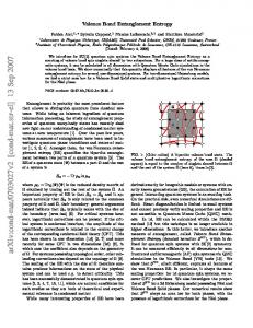
We consider a lattice model composed of two sublattices interpenetrating each other as in Fig. 1, with interaction of infinite range, i.e., every spin interacts with all the other spins in the system, with interaction strength independent of the distance between the spins. Within each sublattice, the interaction is ferromagnetic, and between the sublattices the interaction is antiferromagnetic; as a result there is no frustration. The Hamiltonian is written as, H = −JA
X
i,j∈A
Si ·Sj −JB
X
Si ·Sj +J0
X
Si ,
i,j∈B
X
i∈A,j∈B
Si ·Sj ,
(1) with JA , JB , J0 > 0. The ground state of Eq. (1) can be solved in the following manner[15]. Let SA =
X i∈A
Si ,
SB =
S = SA + SB ,
i∈B
then the Hamiltonian can be written as, 2 2 H = −JA SA − JB SB + J0 SA · SB J0 2 2 2 2 = −JA SA − JB SB + (S 2 − SA − SB ). 2
(2)
Since [S, H] = [SA , H] = [SB , H] = 0, eigenstates of H 2 can be chosen to be simultaneous eigenstates of S 2 , SA 2 and SB , with angular momentum eigenvalues S, SA and
2
FIG. 1: Two-sublattice model: two sublattices labeled A and B interpenetrating each other.
SB respectively, such that the energy eigenvalue is, J0 J0 J0 S(S +1)−(JA + )SA (SA +1)−(JB + )SB (SB +1). 2 2 2 (3) To minimize the energy, we must first maximize SA and SB , and then minimize S, i.e., S = |SA − SB |, SA = NB NA 2 , SB = 2 . Here NA and NB represent the number of corresponding sublattice sites. Physically this means that spins in the same sublattice are all parallel to each other, while spins in opposite sublattices are antiparallel. Thus the ground state is, � NA NB NA NB |SA SB ; Smi = , ; − ,m . (4) 2 2 2 2
In this paper we only consider the simplest case with NA = NB = N , thus the total system size is 2N . Then the ground state is reduced to an antiferromagnetic ground state which has zero total spin, |SA SB ; Smi = |
NN ; 00i. 2 2
(5)
This ground state has perfect Neel order, as manifested by the spin-spin correlation function, 1 , i, j ∈ A or i, j ∈ B; 4 1 1 1 hSi · Sj i = − − → − , i ∈ A and j ∈ B. 4 4N 4 hSi · Sj i =
III.
(6)
THE REDUCED DENSITY MATRIX AND ENTANGLEMENT ENTROPY
We divide the system spatially into two subsystems which are labeled 1 and 2 respectively, as shown in Fig. 2, and study the ground state entanglement entropy E between these two subsystems. E is defined to be the von Neumann entropy of either of the subsystems, E1 or E2 , which can be calculated from the reduced density matrix, E = E1 = E2 = −tr(ρ1 ln ρ1 ) = −tr(ρ2 ln ρ2 ),
(7)
where ρ1 is the reduced density matrix of the subsystem 1, obtained from the density matrix ρ = | N2 N2 ; 00ih N2 N2 ; 00| of the whole system by tracing out degrees of freedom of the other subsystem, ρ1 = tr(2) (ρ), and vice versa.
FIG. 2: Bipartite division of the system. We divide the system spatially in to two parts and label them subsystem 1 and subsystem 2, respectively. One of the main tasks of this paper is to evaluate the entanglement entropy between these two parts.
To solve for the explicit form of the reduced density matrix, we proceed as follows. First, we further decompose the system into four parts, SA1 , SA2 , SB1 , SB2 , with (
P P SA1 = i∈A∧i∈1 Si , SA2 = i∈A∧i∈2 Si ; P P SB1 = i∈B∧i∈1 Si , SB2 = i∈B∧i∈2 Si .
(8)
Therefore, these operators satisfy the following relations, (
SA = SA1 + SA2 , SB = SB1 + SB2 ; S1 = SA1 + SB1 , S2 = SA2 + SB2 .
(9)
Here we note that, as discussed in the previous section, the spin state within each sublattice is ferromagnetic. This means that not only must the total spin quantum numbers of SA and SB take their maximum values, but the total spin quantum numbers of SA1 , SA2 , SB1 and SB2 must also take their maximum values. More importantly, these values are thus fixed, which enables us to treat the operators SA1 , SA2 , SB1 and SB2 as four single spins, and in what follows we shall denote these operators by their corresponding spin quantum numbers. The problem is then that we are given a four spin state in which the spins SA1 and SA2 are combined into a state with total spin SA and the spins SB1 and SB2 are combined in a state with total spin SB , and then these two states are combined into a total singlet (resulting in the ground state of our long-range AFM model), and we must express this state in a basis in which the spins SA1 and SB1 are combined into a state with total spin S1 and SA2 and SB2 are combined into a state with total spin S2 . This change of basis involves the familiar LS-jj coupling scheme. We proceed by first rewriting the density matrix describing the ground state in terms of the basis states |S1 m1 S2 m2 i by appropriate insertions of the unit operator X
S 1 m1 S 2 m2
|S1 m1 S2 m2 ihS1 m1 S2 m2 |,
3 NN NN ; 00ih ; 00| ρ = |SA SB ; SmihSA SB ; Sm| = | 2 2 2 2 X = |S1 m1 S2 m2 ihS1 m1 S2 m2 |SA SB ; Smi
as, p λS1 m1 =(−1)S1 −m1 (2S1 + 1)(2SA + 1)(2SB + 1) SA1 SB1 S1 × SA2 SB2 S1 . SA SB S (14)
S 1 m1 S 2 m2
× hSA SB ; Sm| =
X
S 1 m1 S 2 m2 S1′ m′1 S2′ m′2
X
S1′ m′1 S2′ m′2
|S1′ m′1 S2′ m′2 ihS1′ m′1 S2′ m′2 |
λS1 m1 S2 m2 λ∗S1′ m′1 S2′ m′2 |S1 m1 S2 m2 ihS1′ m′1 S2′ m′2 |, (10)
where λS1 m1 S2 m2 = hS1 m1 S2 m2 |SA SB ; Smi. We then insert another unit operator X
S0 M
|S1 S2 ; S0 M ihS1 S2 ; S0 M |
to express this matrix element as the product of a Clebsch-Gordan coefficient and an LS-jj coupling coefficient[16], hS1 m1 S2 m2 |SA SB ; S mi X = hS1 m1 S2 m2 |S1 S2 S0 M ihS1 S2 S0 M |SA SB Smi S0 ,M
In our case S = 0, so the 9-j symbol can be expressed more simply in terms of a 6-j symbol[18] (see also Appendix B), a b c d e f = δcf δgh (−1)a+d+c+g ((2c + 1))− 12 g h 0 (15) � � 1 a b c × (2g + 1)− 2 . e d g In our particular case, within each sublattice, the state is ferromagnetic, SA = N2 , SB = N2 . Let 2N1 be the size (number of lattice sites) of subsystem 1. Without losing any generality, we can let N1 6 N . Applying Eq. (15) we then have, � N −N N −N � 1 1 p S1 2 2 . λS1 ,m1 = (−1)S1 −m1 (N + 1) N1 N1 N 2
2
2
(16) SA1 SB1 S1 Using a symmetry property of the Racah coefficients[17] = δS0 S δm1 +m2 ,m δM,m hS1 m1 S2 m2 |S1 S2 Smi SA2 SB2 S2 W . (abcd; ef ) = W (acbd; f e), we have, SA SB S � N −N1 � N1 N p (11) 2 2 2 . λS1 m1 = (−1)S1 −m1 (N + 1) N1 N −N1 S1 2 2 (17) SA1 SB1 S1 Then we employ the following relation[17]: Here SA2 SB2 S2 is the LS-jj coupling coefficient or � SA SB S (2a)!(2b)! X-coefficient defined as, W (abcd, a + b, f ) = (2a + 2b + 1)!(c + d − a − b)! (a + b + c − d)!(a + b + d − c)!! l1 s1 j1 × l2 s2 j2 = hl1 l2 s1 s2 LSJM |l1 s1 l2 s2 j1 j2 JM i. (12) (a + f − c)!(a + c + f + 1)!(b + d − f )! �1 L S J (c + f − a)!(d + f − b)(a + b + c + d + 1)! 2 . × (b + f − d)!(b + f + d + 1)!(a + c − f )! Since S = m = 0, we have S1 = S2 , m1 = −m2 . So S1 −m1 (18) √ , and for simplicity, hS1 m1 ; S2 m2 |S1 S2 ; Smi = (−1) 2S2 +1 we can now suppress the S2 and m2 indices and repreThis gives sent λS1 m1 S2 m2 by λS1 m1 without causing any ambiguity. � (N + 1)(N − N1 )!N1 ! Therefore, S1 −m1 λS1 ,m1 = (−1) (N − N1 − S1 )!(N − N1 + S1 + 1)! � 21 S S1 −m1 A 1 SB1 S1 (−1) (N − N1 )!N1 ! √ S S S λS1 m1 = (13) . × 1 . B2 A2 2S1 + 1 S (N1 − S1 )!(N1 + S1 + 1)! A SB S (19) In the following calculation, for consistency, we adopt the convention of Wigner 6-j and 9-j symbols, the definitions of which, and the relation to the Racah coefficients and LS-jj coupling coefficients (or X-coefficients), are given in Appendix A. Following Wigner’s convention, Eq. (13) can be written
Now with the expression above, we can directly trace out the degrees of freedom in subsystem 2 from Eq. (10), with the result X ρ1 = tr(2) (ρ) = (20) |λS1 m1 |2 |S1 m1 ihS1 m1 |. S 1 m1
4 The bipartite entanglement entropy between subsystems 1 and 2 is then given by X E = E1 = − (21) |λS1 m1 |2 ln(|λS1 m1 |2 ). S1 ,m1
Here we note that, although λS1 m1 is written with an explicit m1 dependence, the actual expression is independent of m1 . As a result, we can eliminate the summation over m1 from (21) by multiplying by a factor of 2S1 + 1. The final expression for the entanglement entropy is then X E = E1 = − (2S1 + 1)|λS1 m1 |2 ln(|λS1 m1 |2 ). (22) S1
In the following section we will first derive the asymptotic behavior of the entanglement entropy E in certain limits using the exact results above, and then present the results of our numerical calculation of E with finite system sizes.
IV.
ASYMPTOTIC BEHAVIOR AND ENTANGLEMENT ENTROPY
In this section we consider two limiting cases: (i)N1 = N2 = N , this case gives the saturated entropy at fixed N since intuitively E should increase with the subsystem size. (ii) 1 ≪ N1 ≪ N , in this limit we are considering system’s entanglement with its (much larger) environment, and generically we should be able to find that the entropy should be independent of the total system size as N → ∞, which is indeed what we find. To obtain the asymptotic behavior of the entanglement entropy, we first consider the asymptotic behavior of λS1 m1 , then in the large N limit. Then the summation over S1 which runs from 0 to N/2 can be replaced by an integral. As we will see, the distribution of λS1 m1 is proportional to a Gaussian function with respect to S1 , thus the bounds of integration can be extended to from 0 to +∞. Our concern is the distribution of λS1 m1 with respect to S1 , therefore, we extract the dependence on S1 and P λ2S1 m1 = then use the normalization condition S m 1 1 P 2 S1 (2S1 + 1)λS1 m1 = 1 to obtain the normalization constant. From Eq. (19) we can write, (2N1 )! (N1 − S1 )!(N + S1 + 1)! (2N − 2N1 )! × (N − N1 − S1 )!(N − N1 + S1 + 1)!
λ2S1 m1 ∼
2 S1
(23)
2 S1
∼ e− N1 − N −N1 . This approximation is generally good as long as both N1 and N − N1 are large. In our work, N ≫ 1, and N1 is assumed to be N2 (equal partition) or N ≫ N1 ≫ 1, so
this criteria is satisfied quite well in both cases. Then by the normalization condition X 2 1 1 A(2S1 + 1)e−S1 ( N −N1 + N1 ) S1
≃
Z
∞
(24)
A(2S1 + 1)e
1 + N1 ) −S12 ( N −N 1
1
dS1 = 1,
0
we obtain the (inverse) precoefficient q π(N −N1 )N1 1 ). Therefore, 2 N λ2S1 m1 ≃
N1 −
N12 N
+
1 q
1 2
π(N −N1 )N1 N
1 A
= (N1 − 2 S1
+
2 S1
e− N1 − N −N1 . (25)
The entanglement entropy is therefore given by Z ∞ 2 1 1 E1 ≃ − A(2S1 + 1)e−S1 ( N −N1 + N1 ) 0 � � −S 2 ( 1 + 1 ) × ln Ae 1 N −N1 N1 dS1 ! r N12 1 π(N − N1 )N1 . ≃ ln N1 − + N 2 N A.
N12 N
(26)
Equal Partition
Here for simplicity we set N even (note that the total system size is 2N ), thus N1 = N2 = N/2, and A1 = √ 1 N π), then 4 (N + 2 4S1 4 √ e− N , N + Nπ and the entanglement entropy becomes, � � 1√ N + E = ln πN 4 4 ≃ ln N − ln 4 ≃ ln N − 1.38629.
λ2S1 m1 =
(27)
(28)
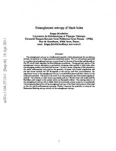
Compared with our numerical result, as shown in Fig. 3, we see that they agree very well, not only for the prefactor of the ln N dependence, but the intersection coefficient as well. B.
Unequal Partition
In this case, 1 ≪ N1 ≪ N , we can expand the entropy as follows, s π(1 − NN1 ) 1 N 1 + E ≃ ln N1 1 − N 2 N1 s π(1 − NN1 ) N 1 1 (29) = ln N1 + ln 1 − + N 2 N1 � �2 ! N1 N1 . +O ≃ ln N1 − N N
5 10 8 6
Entanglement Entropy
Entanglement Entropy
Numerical Calculation Asymptotic Behavior E = lnN - ln4 Fit line for Numerical Calculation E = 0.99983 lnN-1.0227
4 2 0 10
100
1000
N =10
2.5
1
N =8 1
N =6 1
N =4
2.0
1
N =2 1
N =10 1
1.5
N =8 1
N =6 1
N =4 1
1.0
N =2
10000
1
0
N
50
100
150
200
N
From this expression we see that when the assumed condition is satisfied the entropy indeed depends only on the subsystem size to leading order. To check to what extent our approximation is still valid, we plot the expression as a function of total system size N with different subsystem size N1 , as shown in Fig. 4. This figure shows that when N is large enough the entropy becomes independent of N , and the first order term, ln N1 dominates except for an apparently constant shift from the exact curve. We have also plotted the asymptotic behavior as a function of N1 while keeping N fixed, shown in Fig.5.
V.
FERROMAGNETIC MODEL AND ITS ENTANGLEMENT ENTROPY
FIG. 4: (Color online) Comparison of asymptotic behavior (solid line) and exact numerical calculation (scattered points) of entanglement entropy E. As total system size N increases, E tends to a constant for a fixed subsystem size N1 , as expected. Difference between them increases as the subsystem size increases, as the condition 1 ≪ N1 ≪ N/2 gets less satisfied.
12 Entanglement Entropy
FIG. 3: (Color online) Comparison of asymptotic behavior (black solid line) and exact numerical calculation (scattered points) of entanglement entropy E. Exact calculation of E for the equal partition case is compared with asymptotic behavior we derived in the text up to N = 10000. Results obtained from these two methods agree well. Our approximation of the asymptotic behavior gives E ≃ ln(N ) − 1.38629, compared with the best fit line (red dashed line) E = 0.99983 ln N − 1.0227.
Numerical Calculation
10
Asymptotic Behavior : E = ln N 1
Best Fit: 0.61435+0.93753 lnN
8
Asymptotic Behavior with Correction: E = ln N
- N /N 1
1
6 4 2 0 1
10
100
1000
10000
N 1
In this section we consider a ferromagnetic (FM) spin1/2 model on an arbitrary lattice with N sites, H=−
X i6=j
Jij Si · Sj ,
(30)
with Jij > 0. The ground state is the fully magnetized state |SM i with S = N/2 and M = −S, −S + 1, · · · , S, and is clearly long-range ordered: hSi · Sj i = 1/4. However there is a crucial difference between the FM ground state and the AFM ground state studied earlier: the FM ground state has a finite degeneracy, and thus the system exhibits a non-zero entropy even at zero temperature, E0 = log(2S + 1) = log(N + 1), resulting from the
FIG. 5: (Color online) Asymptotic behavior of entanglement entropy E as function of N1 with N fixed (solid blue line). Here N = 10000. Compare it with the scattered points, which are an exact numerical calculation of E. We find the asymptotic behavior is accurate until N1 becomes comparable to N . We also plot the asymptotic behavior with first order correction(dashed light green line) which exhibits the correct tail effect when N1 becomes comparable with N .
6 density matrix of the entire system,
and E1 = ln(N1 + 1) (in agreement with Ref. [14]). Similarly E2 = ln(N2 + 1). Thus
S X 1 |SM ihSM | 2S + 1
ρ=
E = [ln(N1 + 1) + ln(N2 + 1) − ln(N + 1)]/2.
M=−S
S X 1 |SM ihSM | N +1 M=−S 1 0 ... 0 1 0 . 1 . . 0 1 0 = N +1 . .. ... 0 1
=
(31)
ρ1 = tr(2) ρ =
lim E →
VI.
S X 1 tr(2) (|SM ihSM |) N +1 M=−S
=
1 N +1
S X
ρ1M ,
M=−S
S X 1 tr(1) (|SM ihSM |) ρ2 = tr(1) ρ = N +1
(32)
M=−S
=
1 N +1
S X
ρ2M ,
M=−S
and calculate from them the entropy of the subsystems, E1 and E2 . The entanglement entropy is defined as[20] E = (E1 + E2 − E0 )/2.
(33)
For the present case E1 and E2 can be easily obtained from the following observations. (i) Because the total spin is fully magnetized, so are those in the subsystems: S1 = N1 /2 and S2 = N2 /2. Thus this is a two-spin entanglement problem. (ii) Because the total density matrix ρ is proportional to the identity matrix in the ground state subspace, it is invariant under an arbitrary rotation in this subspace. (iii) As a result the reduced density matrix ρ1 is also invariant under rotation in the subspace of subsystem 1 with S1 = N1 /2, and is proportional to the identity matrix in this subspace. Thus N1
1 ρ1 = N1 + 1
2 X
M1 =−
N1 2
|
N1 N1 M1 ih M1 | 2 2
1 0 ... 0 1 0 0 1 0 1 , = N1 + 1 .. .. . . ... 0 1
We find in both the equal partition (N1 = N2 = N/2, here again we set N even for simplicity) and unequal partition (N1 ≪ N2 = N − N1 ) limits, the entropy grows logarithmically with subsystem size N1 , N1 →∞
In this case the entanglement entropy between two subsystems (1 and 2) is defined in the following manner. We first obtain reduced density matrices for subsystems 1 and 2 by tracing out degrees of freedom in 2 and 1 from ρ:
(34)
(35)
1 ln(N1 ). 2
(36)
CONCLUDING REMARKS
In this paper we have studied antiferromagnetic (AFM) and ferromagnetic (FM) spin models with perfect long-range magnetic order in their ground states, and calculated the ground state block entanglement entropy when the system is divided into two subsystems (or blocks). In both cases we find the entropy grows logarithmically with block size. In the following we discuss the significance of our results. First of all, there is entanglement, despite the perfect long-range order in the ground state. This is somewhat surprising as one might think that in such Hamiltonians one can obtain certain properties of the system exactly using mean-field theory, in which the ground state is approximated by a product state with no entanglement. Our results indicate that mean-field approximation is not appropriate for entanglement calculation, even if it is “exact” for other purposes. This point is particularly striking for the AFM model, in which the ground state is unique. The source of the discrepancy is there still is quantum fluctuations even in such a model with super long-range interaction, which render the ground state a singlet, even though quantum fluctuation does not reduce the size of the order parameter. The entanglement is due to the quantum fluctuation of the direction of the order parameter, which is a collective mode with zero wavevector (or a zero mode); this is missed by any mean-field approximation. Secondly, the entropy does not obey the area law. The reasons for that are different for the two cases we studied. In the AFM model, the interaction does not depend on distance in the Hamiltonian, thus there is no notion of distance or area in this model. In the FM model, on the other hand, the ground state is independent of the Hamiltonian, as long as all interactions are FM. The fully magnetized ground states are invariant under permutation of spins, thus there is no notion of distance or area in the ground states, even though the terms in Hamiltonian can have distance dependence. Thirdly, the absence of an area law is special to the cases we studied, again each in their own ways. For the FM model, it is specific to zero temperature. As soon as a finite temperature is turned on, one expects the entanglement entropy (or mutual information) to grow
7 with the area separating the two subsystems or blocks, as long as the interaction is not long-ranged[22]. For the AFM model at zero temperature, we do expect an area-law contribution to the entropy for short-range or even certain power-law long-ranged interaction due to quantum fluctuations. This is most easily seen within spin-wave approximation, which is a version of meanfield theory. Within the spin wave approximation spins are mapped onto bosons, and the Hamiltonian is mapped onto coupled harmonic oscillators. Detailed recent studies have established the area law of entanglement for such systems[4]. In this regard the super long-range AFM model we study here is very special, in that all spin-wave degrees of freedom at finite wave-vector disappear, and the only degrees of freedom contributing to the ground state are zero wave-vector modes represented by SA and SB [15]; as a result there is no area-law contribution from quantum fluctuations of spin-waves. We conclude by speculating that in the more general cases that do have an area-law contribution to the entanglement entropy, as long as long-range spin order is present, the logarithmic contribution due to fluctuations of the order parameter zero-modes we find here will remain and show up as a sub-leading (yet singular) correction to the area law. If that is the case, then conventional long-range order contributes to the entanglement entropy in a way similar to the much subtler topological order[7, 8] or quantum criticality[9].
Acknowledgments
We acknowledge support from National Science Foundation grants No. DMR-0225698 and No. DMR-0704133 (W.D. and K.Y.), State of Florida (W.D.), and US DOE Grant No. DE-FG02-97ER45639 (N.E.B.).
APPENDIX A
6-j Symbol & Racah coefficient: � � j1 j2 J12 = (−)j1 +j2 +j3 +J W (j1 j2 Jj3 ; J12 J23 ) j3 J J23 1
= (−1)j1 +j2 +j3 +J [(2J12 + 1)(2J23 + 1)]− 2 × hj1 , J23 ; J|J12 , j3 ; Ji.
(A1)
where J12 and J23 refer to the coupling of j1 and j2 or j2 and j3 respectively.
9-j Symbol & LS-jj Coupling coefficient:
a b c d e f = ((2c + 1)(2f + 1)(2g + 1))− 21 g h i a b c 1 × (2h + 1)− 2 d e f g h i
(A2)
1
= ((2c + 1)(2f + 1)(2g + 1)(2h + 1))− 2 × h(ab)c, (de)f ; i|(ad)g, (bc)h; ii.
APPENDIX B
In this Appendix we give a slightly simplified derivation of the entanglement entropy for the singlet ground state of the infinite-range AFM model defined in Sec. II. While this derivation is not as general as that given in the main text (which can, in principle, be applied to states with nonzero total spin), it has the advantage of clarifying the reason for the appearance of the Wigner 6jsymbol in the final result for the entanglement entropy. Following the notation of Sec. II and III, we consider the case of 2N spin-1/2 particles divided equally into two sublattices A and B. The spins on each sublattice are taken to be fully polarized, so that SA = N/2 and SB = N/2. In what follows we will use a notation in which, for example, the state for which the spins SA and SB form a singlet is represented as (SA , SB )0 . In this notation, pairs of spins contained within a set of parenthesis form a state whose total spin is equal to the subscript labeling the parenthesis. Thus, (SA , SB )0 is a singlet state equivalent to the state defined in Eq. (5) in Sec. II. (Needless to say, for this state to exist it is necessary to have SA = SB .) Now we consider what happens if these spins are divided into two different subsystems labeled 1 and 2. Following Sec. II, if SAi is the total spin quantum number of the A sublattice spins in subsystem i = 1, 2, and SBi is the total spin quantum number of the B sublattice spins in subsystem i = 1, 2, then the state of the spins on the A sublattice can be written (SA1 , SA2 )SA and the state of the spins on the B sublattice can be written (SB1 , SB2 )SB . The total singlet state for the entire system, |ψi, can then be expressed as |ψi = (SA1 , SA2 )SA , (SB1 , SB2 )SB
�
0
.
(B1)
Note that we have not included the m quantum numbers associated with the z-components of SA and SB in writing the above expression for |ψi. This is not necessary because the requirement that the total spin of the two sublattices combine to form a singlet uniquely determines the state. It should, of course, always be understood that when we write Eq. (B1) what is really meant
8 (in obvious notation) is,
(see Appendix A).
SA X 1 (−1)m | (SA1 , SA2 )SA ; mi |ψi = √ 2SA + 1 m=−S A
⊗ | (SB1 , SB2 )SB ; −mi.
Rearranging the spins again, and using the fact that the total spin of all four spins is 0, we can express the resulting four spin basis states as follows,
(B2)
Equation (B2) effectively (up to irrelevant phase factors) gives the Schmidt decomposition (see, e.g., [1]) of the state |ψi into the two subsystems consisting of the A and B sublattices. Given such a Schmidt decomposition it is straightforward to determine the entanglement between these two subsystems. However, here we are interested not in the trivial entanglement between subsystems A and B, but the entanglement between subsystems 1 and 2. To find this we need the Schmidt decomposition of |ψi into subsystems 1 and 2. Note that because |ψi is a total spin singlet it follows that � |ψi = (SA1 , SA2 )SA , (SB1 , SB2 )SB 0 � � = ((SA1 , SA2 )SA , SB2 )SB , SB1 , (B3) 1
0
where, for convenience, we have rearranged the order of the spins in the second equality. The key point here is that the three spins SA1 , SA2 and SB2 must be in a state which is a total spin eigenstate with total spin SB1 . If this were not the case it would be impossible to form a total spin singlet with the remaining spin SB1 . Next we use the Wigner 6j-symbol to express the three spin state ((SA1 , SA2 )SA , SB2 )SB as a superposition of 1 � states of the form SA1 (SA2 , SB2 )S2 S . The result is
�
SA1 (SA2 , SB2 )S2
(SA1 , SA2 )SA , SB2 S B1 X � N = (−1) γS2 SA1 , (SA2 SB2 )S2 S S2
B1
, (B4)
where the coefficients are given by � � p S A1 S A2 S A γS2 = (2SA + 1)(2S2 + 1) , (B5) SB2 SB1 S2
[1] M.A. Nielsen, I.L. Chuang, Quantum Computation and Quantum Information (Cambridge University Press, Cambridge, UK, 2000). [2] Luca Bombelli, Rabinder K. Koul, Joohan Lee, and Rafael D. Sorkin, Phys. Rev. D 34, 373 (1986). [3] Mark Srednicki, Phys. Rev. Lett. 71, 666 (1993). [4] For a review, see Luigi Amico, Rosario Fazio, Andreas Osterloh, and Vlatko Vedral, arXiv:quant-ph/0703044. [5] Michael M. Wolf, Phys. Rev. Lett. 96, 010404 (2006); D. Gioev, and I. Klich, Phys. Rev. Lett. 96, 100503 (2006). [6] C. Holzhey, F. Larsen, and F. Wilczek, Nucl. Phys. B 424, 443 (1994); G. Vidal, J. I. Latorre, E. Rico, and A. Kitaev, Phys. Rev. Lett. 90, 227902 (2003); P. Cal-
SB1
, SB1
�
0
= (SA1 , SB1 )S1 , (SA2 , SB2 )S2
�
0
(B6)
where, obviously, S1 = S2 . We therefore conclude that |ψi = (−1)N
X
γS2 (SA1 , SB1 )S2 , (SA2 , SB2 )S2
S2
�
0
.(B7)
Finally, after writing the m sum explicitly (as in Eq. (B2)), we have the desired Schmidt decomposition (again, up to irrelevant phases) of the state |ψi into subsystems 1 and 2,
N
|ψi = (−1)
S X X
S m=−S
(−1)m λSm | (SA1 , SB1 )S , mi
⊗ | (SB2 , SA2 )S , −mi
(B8)
where
B1
�
�
λSm
� � p S A1 S A2 S A = 2SA + 1 . SB2 SB1 S2
(B9)
When the values of SA = N/2, SA1 = SB1 = N1 /2, SA2 = SB2 = (N − N1 )/2 are substituted into this expression it can be seen to be equivalent to that given in Eq. (16) in Sec. III. The derivation of the entanglement entropy given in the main text follows.
abrese and J. Cardy, J. Stat. Mech. (2004) P06002; G. Refael and J.E. Moore, Phys. Rev. Lett. 93, 260602 (2004); R. Santachiara, J. Stat. Mech.: Theory Exp., L06002 (2006); Adrian Feiguin, Simon Trebst, Andreas W. W. Ludwig, Matthias Troyer, Alexei Kitaev, Zhenghan Wang, Michael H. Freedman, Phys. Rev. Lett. 98, 160409 (2007); N. E. Bonesteel and K. Yang, Phys. Rev. Lett. 99, 140405 (2007). [7] Alexei Kitaev and John Preskill, Phys. Rev. Lett. 96, 110404 (2006). [8] M. Levin and X.-G. Wen, Phys. Rev. Lett. 96, 110405 (2006). [9] Eduardo Fradkin and Joel E. Moore, Phys. Rev. Lett.
9 97, 050404 (2006). [10] Jos´e I. Latorre, Rom´ an Or´ us, Enrique Rico, and Julien Vidal, Phys. Rev. A 71, 064101 (2005). [11] Thomas Barthel, S´ebastien Dusuel, and Julien Vidal, Phys. Rev. Lett. 97, 220402 (2006). [12] Julien Vidal, S´ebastien Dusuel and Thomas Barthel, J. Stat. Mech. P01015 (2007). [13] The entanglement property of this model has bee previosuly studied in Ref.14. Here we introduce a different definition of the entanglement entropy that properly takes into account the ground state degeneracy, and can be calcualted much more straigtforwardly using symmetry consideration. See Sec. V. [14] V. Popkov and M. Salerno, Phys. Rev. A 71, 012301 (2005). [15] Eddy Yusuf, Anuvrat Joshi, and Kun Yang, Phys. Rev. B 69, 144412 (2004). [16] V. Devanathan, Angular Momentun Techniques in Quantum Mechanics, Kluwer Academic Publishers, 2002. [17] D. M. Brink, G. R. Satchler, Angular Momentum, Appendix II, Second Edition, Oxford University Press, 1968. [18] D. M. Brink, G. R. Satchler, Angular Momentum, Ap-
[19] [20]
[21] [22]
pendix III, Second Edition, Oxford University Press, 1968. W. Beckner, Pearson, Bull. London Math. Soc. 30 , 80 (1997). This definition is probably not unique. It is one half of the “mutual information” introduced in Ref. 21, 22, and reduces to Eq. (7) when ρ is that of a pure state. The same definition was used by Castelnovo and Chamon [Claudio Castelnovo, and Claudio Chamon, Phys. Rev. B 76, 174416 (2007)]. The name “mutual information” may be first coined by Adami and Cerf [C. Adami and N.J. Cerf, Phys. Rev. A 56, 3470 (1997)] and Vedral, Plenio, Rippin and Knight [V. Vedral, M.B. Plenio, M.A. Rippin, and P.L. Knight, Phys. Rev. Lett. 78, 2275 (1997)], although Stratonovich [R. L. Stratonovich, Izv. Vyssh. Uchebn. Zaved., Radiofiz. 8, 116 (1965); Probl. Inf. Transm. 2, 35 (1966)] considered this quantity already in the mid-1960s. M. Cramer, J. Eisert, M. B. Plenio, J. Dreissig, Phys.Rev. A 73, 012309 (2006). M. M. Wolf, F. Verstraete, M.B. Hastings, and J.I. Cirac, Phys.Rev.Lett. 100, 070502 (2008).