Experiments with synthetic images and Cephalograms are described. 1. Introduction. Many image analysis tasks can be carried out by making inferences from ...
Boundary Detection Using Bayesian Nets N. Bryson and C. J. Taylor Department of Medical Biophysics, University of Manchester, Oxford Road, Manchester MI3 9PT.
Abstract This paper describes the application of Bayesian networks to the generation of explanations for the evidence provided by one or more 1-D profiles. Experiments with synthetic images and Cephalograms are described.
1. Introduction Many image analysis tasks can be carried out by making inferences from the evidence available in 1-D profiles taken from selected parts of the image, combined with constraints defined by the user, and possibly estimated from a training set [1,2]. A fundamental task is thus to label segments of the profile as being "explained" by the presence in the scene of objects drawn from predefined classes.
2. Bayesian Networks A Bayesian net consists of nodes, representing variables or sets of mutually exclusive hypotheses, and directed links between the nodes, representing constraints between the variables. Normally the net is sparsely linked, since variables are only influenced or have a causal connection with a limited set of other variables[3]. Associated with each node is a probability distribution over the variable, and a conditional probability distribution over the "parents" of the node, (where parents and children are defined by the direction of the link joining them). Receipt of evidence about any variable causes a revision in our belief in other variables via likelihood distributions, using the conditional probabilities and Bayes theorem, as described below.
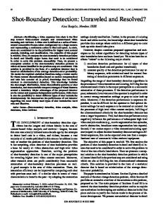
2. 1. A Bayesian Net for Multiple Segments The basic building block of a profile explanation is derived from the grey level model of an object class, which is used to explain one segment of the profile. Figure 1 represents part of a network representing a multi-segment model.The boxes containing P and S; represent the sets or spaces of hypotheses: The current profile is p and The i-th segment of the profile is st. X{ represents the set of hypotheses: The end of the segment explained by the grey level model G, lies a distance x; pixels along the profile, where xtis an integer in the range [0,,/v-l]. The box containing G, represents the set of hypotheses : The grey level model is characterised
23
by the vector ofparameters & , where for example & could be the mean and standard deviation of a Gaussian distribution. The grey model & explains the grey-level evidence on the segment *, between ^., and %.
Figure 1 - Bayesian net
2. 2. Shape and Grey level Constraints The arrows connecting the variables in figure 1 represent constraints, such as the requirement that each segment have a different object label, constraints on the width of each segment and probabilistic models of the grey-level distribution on each segment.
3. Network Transformation Several techniques are suggested by Pearl [4] for the simplification and solution of multiply-connected nets - clustering of variables, instantiation of selected variables[5], and stochastic sampling. The first two techniques render the net singly-connected, which allows a solution to be constructed by replacing the optimisation by a sequence of nested optimisations, as described in the next section. In this paper we proceed by introducing a compound variable Zj = Gt ® Si ® Xi and by instantiating p to each of its possible values, producing the network shown in figure 2. The set \Zt : i - 1,...,/) represents the unknowns on the segments, and the set {P, : i = 1,...,/] represents the evidence applied to each segment. 7
7
ii
i
1
Pi-i
Pi
1
P,«
Figure 2 - Singly connected net
24
4. Belief Revision The space of all possible solutions is defined by the variable w - z, ® ft ® z 2 ® p2 ® ... ® z, ® ft. We seek the most probable member w' ew, given the evidence e e £ - Pt ® P2 ® .... ® ft, i.e. /K^'IO ~ rnaxp(w\e)
(1 )
w
We can exploit the single-connectivity of the net to recursively decompose this expression. Using the notation W - W~ ® Z, ® W? , and E - Ej ® ft ® E* where w~ - Z! ® Pi ® ... ® ZM ®
ft_i
and
w* — zi+i ®ft+i® ... ® z ; ® p,,
then maxp(iv | e) = ^ maxl^ (21 ) ^ (z, )]
O "\
where ., (z,.,
a,
(3) (4)
The n, and Ai functions represent causal and evidential support for each value of Zi. Effectively, each variable selects its optimal value (constrained by the optimal values selected by other variables) by assembling optimal sub-explanations from each sub-net connected to it. By combining these the variable is able to assemble optimal sub-explanations for larger sub-nets, which are then passed to its neighbours in the net.
z\
z\
\
\
^
Zi
\ p\
P!
A
z\
\
\
P3
z| \ Pi
P?
P5
\
z\
z\ \ \
z]
V\ P!
^.
V\ P!
Pi
Figure 3 - Singly connected net representing three profiles
25
5. A Multi-profile Net The single profile model can be extended to a multi-profile model, representing profiles across a putative boundary, with constraints between the first segments of each profile, as shown in figure 3. Various constraints, expressed as conditional probabilities /Kzi+Vi ) are used, ranging from a weak constant grey model constraint, through a continuity constraint to a strong vertical edge constraint. The belief updating procedure can be derived in a similar manner to that shown above.
> - /.
'-&%
.v*...
Figure 4 - Synthetic image
Figure 5 - Single profile net result
Figure 6 - Constant grey model result Figure 7 - Continuity constraint result Multiple-profile nets have been applied along selected boundaries of the synthetic image shown in figure 4. This image consists of regions whose pixel values have been drawn from Gaussian populations with equal variances and differing means. After training, sets of adjacent, horizontal profiles were extracted across the boundaries between the regions, and processed by the net shown in figure 3. Figures 5-8 show the results of applying no constraint (single profile nets), the constant grey model constraint, the continuity constraint and the vertical edge constraint, respectively. The profiles have been colour-coded to show the labelling of segments and the location of segment boundaries. Note the improvement in location of the edges as the constraint is made stronger.
26 1
0.8 0.6
• •
0.4
- p(A |AB ) -p(B|AB)
0.2
0 0.4
Figure 8 - Vertical edge constraint result
0.6 s/n
0.8
Figure 9 - Typical mis-labelling rates
6. Sensitivity and Localisation The performance of an edge detector is characterised by its ability to detect the presence of an edge (the sensitivity), and the ability to accurately locate the edge. We considered images containing vertical stripes, 64 pixels wide, drawn from two Gaussian populations, A and B, with equal variances. We can express the sensitivity of the net by evaluating, at several signal-to-noise ratios, a "confusion" matrix, consisting of elements of the form p(A\XB) where the characters in bold represent the true labelling of the evidence. Below a certain signal-to-noise ratio the net misclassifies masks containing edges as pure A or B regions, because sizeable fluctuations in A (or B) are more likely to explain the evidence than the presence of an edge. A typical result is shown in figure 9. However, if more profiles are used, a point is reached where the weight of evidence becomes too large to be explained away as a fluctuation. pixels
-0.5
Figure 10 - Localisation accuracy Figure 11 - Localisation precision The ability of the Bayesian net shown in figure 3 to locate an edge was examined by using the same set of images as above. The net was constrained to find an edge by feeding it with a priori, distribution which disallows values JC, a N, but is otherwise uniform. The relative widths of the profiles and the stripes ensures
27
that only one edge will be found. The accuracy of the edge location can be defined as the mean of the localisation error, and the precision is defined as the standard deviation of the localisation error. These are shown in figures 10 and 11. As might be expected, the accuracy and precision increase as the signal-to-noise ratio increases.
7. Edge Location in Cephalograms The work of Davies [6] concerns the automatic location of key features in cephalograms, such as that shown in figure 12. In particular, the chin is often difficult to locate (because of the imaging technique), although hitlines which straddle this region can be reliably planted.
Figure 12 - Cephalogram with detected Figure 13 - Model of the chin region chin marked A simple model of the image is shown in figure 13. Region A is the dark background, B is the grey bone area (which can often appear indistinguishable in appearance from region A), and region C is the tooth. The boundary of interest is that between regions A and B or A and C. We can represent this using the Bayesian net shown in figure 3, with profiles numbered from the bottom of the image.The shape constraint is imposed using a modified version of the continuity constraint. The net was trained on twenty examples, and found the chins on five unseen examples, one of which is shown in figure 12 with the detected chin marked.
8. Discussion Bayesian nets allow us to generate and train customized masks for boundary detection. The architecture of the net shown in figure 3 is applicable to a variety of detection problems, since it allows us to model the appearance of the boundary and adjacent regions. We are able to incorporate constraints on the shape of the boundary, and on the legality of various labellings of adjacent regions. The results shown in figures 5-8 indicate that use of such constraints cause a significant improvement in performance.
28
Singly-connected nets were developed to allow the use of Pearl's belief revision algorithm, but in any realistic case the constraints are more suitably modelled by a multiply-connected net [5]. A variety of relaxation labelling algorithms are available for such problems [7,8] but have the disadvantage that we lose the theoretical justification provided by statistical decision theory. The most severe difficulty with the current algorithm is that computational effort is expended on generating accurate sub-explanations for all possible values of a variable, irrespective of whether that value is likely to be needed. Since the evaluation of one of the 20x40 pixel masks used in the "chins" examplar takes about 90 seconds on a Sun 3/160, we must find solution techniques which direct computational effort towards likely explanations. There is scope for carrying out the processing in parallel, since.within each node, the evaluation of the A, n and belief functions can be evaluated in parallel.
9. Conclusion We have generated Bayesian nets to represent boundary regions for a mixture of synthetic and real images. The belief revision algorithm was outlined, and experiments on the synthetic images have illustrated the properties of the net under a variety of signal-to-noise ratios, and with a variety of boundary shape constraints. The net has also been used to model the appearance of a region of a set of real-world medical images.
REFERENCES [1] Cooper D.H., Bryson N., Taylor C.J., An Object Location Strategy using Shape and Grey-level Models, Image and Vision Computing 1, 1, 50-56 (1989) [2] Woods P.W., Taylor C.J., Cooper D.H., Dixon R.N., The use of geometric and grey-level models for industrial inspection, Pattern Recognition Letters, 1 (1987) 11-17 [3] Shacter R.D., Probabilistic Inference and Influence Diagrams, Op. Res., 26, 4, pp 589-604 (1988) [4] Pearl Judea, Probabilistic Reasoning in Intelligent Systems:- Networks of Plausible Inferences, Morgan Kaufmann Publishers Inc. [5] Suermondt H.J., Cooper G.F., Probabilistic Inference in Multiply Connected Belief Networks Using Loop Cutsets, Int. J. Approx. Reasoning, 4, 283-306 (1990) [6] Davis, D. N., Taylor C.J., An Intelligent Visual Task System for Lateral Skull X-ray Images, Procceedings of the British Machine Vision Conference (Oxford) 291-295, September 1990 [7] Hummel R.A., Zucker S.W., On the Foundations of Relaxation Labeling Processes, IEEE Trans. PAMI-5,3,267-286, May 1983 [8] Kittler J., Illingworth J., Relaxation labelling algorithms - a review , Image and Vision Computing 3,4,207-216 November 1985