BRAND CHOICE MODELS
Gary J. Russell Henry B. Tippie Research Professor of Marketing Tippie College of Business University of Iowa
Citation Information
Russell, Gary J. (2014), “Brand Choice Models” in Russell Winer and Scott A. Neslin (eds.), The History of Marketing Science, Hanover, MA: Now Publishers, 19-46.
Contact Information Professor Gary J. Russell S350 Pappajohn Business Building, Tippie College of Business, University of Iowa, Iowa City, IA 52242 Email Address:
[email protected]
INTRODUCTION The theory of brand choice is one of the fundamental elements of marketing science. Virtually all decisions made by marketing managers involve assumptions – explicit or implicit – about how consumers make purchase decisions and how strategic marketing variables (such as price, advertising and distribution) impact these decisions. To support this effort, the goal of research in brand choice is to create models that both reflect the behavioral realities of consumer choice and allow accurate forecasts of future choice behavior. The history of research in brand choice is a complex blend of research drawn from psychology, economics and statistics. Because brand choice covers a large number of distinct topics, it is best to think of the area in terms of a slow evolution from fundamental research in psychology in the 1950’s to applied micro-economic theory in the 2000’s. In Figure 1, we have organized this evolution under six general research themes: Theoretical Foundations, Single Choice, Consumer Heterogeneity, Multiple Decisions, Economic Theory, and Choice Dependence. These headings are listed in rough chronological order, with arrows denoting paths of influence. For the most part, the arrows are intended to show the relationships between subtopics, not between individual articles. However, it should be understood that chronology is important: earlier work almost always informs later work. For example, research on logit models (in the 1980’s) and on consumer response parameter heterogeneity (in the 1990’s) made possible later work on spatial choice (in the 2000’s). This chapter is not a detailed review of work in brand choice over the last 50 years. Readers interested in detailed discussions of early work in brand choice should consult Massy et al. (1970) (stochastic brand choice) and Corstjens and Gautschi (1980) (economics and psychology). Readers interested in a comprehensive examination of the impact of economic theory on the evolution of choice modeling should consult Chandukala et al. (2007). This chapter is organized as follows. Using Figure 1 as a guide, we first review (in chronological order) the six general research themes in brand choice. Within each theme, we discuss various subfields, noting interrelationships. As will be seen, this discussion illustrates the fact that improvements in data availability and statistical tools have repeatedly stimulated new work in choice theory and new application areas. We conclude with a brief discussion of possible future developments in brand choice. THEORETICAL FOUNDATIONS Brand choice models rest upon key assumptions about how consumers make purchase decisions. In contrast to research by psychologists in marketing, theories in choice modeling are not intended to be process models detailing how the organization of the human brain leads to choice outcomes. Rather, theories in choice modeling are artificial in the sense of Simon (1969): they are paramorphic (“as if”) representations of choice behavior designed to improve our understanding of the impact of environmental influences (such as the marketing mix) on choice decisions. In this section, we review pioneering work in psychology that set the stage for future developments. Definition of a Choice Model We define a choice model in the following manner. A consumer is presented with the task of selecting one of N alternatives, denoted A(1), …. , A(N). For each alternative, the exists a mapping from the characteristics of each alternative to a real-valued number V(A(i)) = V(i). The consumer constructs U(V(i)) = U(i), called preference (psychology) or utility (economics), which allows an ordering of the alternatives on a one-dimensional continuum. Using the U(i) values, the consumer selects one alternative by employing some type of decision rule. The decision rule assigns a probability of choosing alternative i as Pr(i) = F(U(1), …, U(N)) where 0 < Pr(i) < 1 and F(.) is some multivariate function with N arguments. That is, the choice process is assumed to be inherently stochastic: there is no alternative with Pr(i) = 0 or Pr(i) = 1.
2
Although this definition may seem needlessly formal, it provides the researcher important guidelines for developing a choice model. Clearly, three elements are needed: a set of choice alternatives, a set of corresponding U(i) preference scale values, and a decision rule. The history of brand choice can be viewed as an evolving understanding of how these components ought to be specified in marketing applications. Thurstone Model The starting point for brand choice is the work of Louis Thurstone, a psychologist interested in psychophysics (the human perception of physical stimuli such as the intensity of light). His experiments required subjects to determine which of two stimuli was more intense (e.g., which light was brighter). His key insight, reported in his Theory of Comparative Judgment (Thurstone (1927), reprinted in Thurstone (1959)), is that humans do not perceive a stimulus in the same fashion on different occasions, even though the stimulus object has not changed. Using our earlier notation, Thurstone postulated a discriminal process of the form U(i) = V(i) + e(i)
(1)
where V(i) is the true intensity of A(i), and e(i) is a normally distributed random variable with mean zero. That is, U(i) is the sensation of intensity that is perceived by the individual and is used to decide which stimulus has higher intensity. Thurstone argued that the choice rule is simple: the subject selects the stimulus with the higher U(i) value. Because the e(i) error varies across stimuli and over time, Thurstone’s model implies that judgments of intensity made by one individual will be inconsistent, particularly when the true V(i) values are similar. As such, a researcher can only predict the probability that a certain alternative will be judged to be most intense. In a brand choice setting, V(i) is interpreted as the long-run average preference value of the alternative and e(i) is a situation-specific random effect that masks the relationship between the true V(i) value and perceived U(i). Following Thurstone (1927), researchers in marketing assume that the consumer always chooses the alternative with highest perceived U(i). This combination of a randomly generated U(i) value coupled with a (deterministic) maximum U(i) choice rule is today known as a random utility theory (RUT) model. Choice probabilities for a RUT model are obtained by writing down the N-dimensional multivariate distribution defined by equation (1) and then computing the probability Pr(i) = Pr{U(i) = max [U(1), …, U(N)]}. (See Train (2003) for details.) When the e(i) are normally distributed (as assumed by Thurstone (1927)), the resulting choice process is known as a probit choice model. Luce Model Luce (1959) proposed an alternative theory of choice based upon certain assumptions about choice probabilities. Let Pr(i|S) denote the probability of selecting item i from S, a set of alternatives including both item i and another item j. Let S* be another set of items, also including both i and j. Luce’s Choice Axiom takes the form Pr(i|S)/Pr(j|S) = Pr(i|S*)/Pr(j|S*)
(2)
In words, the Choice Axiom states that the ratio of choice probabilities is a fixed quantity that does not depend upon the choice set. Choice models with this property are said to exhibit independence from irrelevant alternatives. Luce (1959) shows that equation (2) is sufficient to derive an explicit expression for the choice probabilities. If the Choice Axiom holds, then there exists a ratio-scaled preference value Q(i) for each item. Moreover, relative to a set of alternatives S = {A(1), …, A(N)}, Pr(i|S) = Q(i)/{Q(1) + … + Q(N)}
(3) 3
Luce (1959) argues that Q(i) represent psychologically-real preference values that are fixed over time. Accordingly, the stochasticity of choice (and the need for choice probabilities) is due to errors made in the decision process. The probability function in equation (3) is called a logit choice model in academic marketing. Logit models dominated the choice theory literature in marketing science during the 1980’s. One key reason is that the model is computationally tractable, even for large choice sets. However, an equally important reason is that logit models are also RUT models. Yellott (1977) showed that logit choice probabilities are consistent with a RUT model in which the e(i) are independent draws from an extreme value distribution. Relative to equation (1), the Luce preference values depend upon RUT utilities according to the expression Q(i) = exp(V(i)), where exp(.) denotes the exponential function. Moreover, McFadden (1980) showed that the logit model can also be derived using a micro-economic argument based upon RUT. (In the economic interpretation of the logit model, the e(i) errors represent variables that impact choice, but are not observed by the researcher.) The popularity of the logit model is due in large part to these connections to theories in both psychology and economics. Tversky Models Amos Tversky made major contributions to choice theory that stimulated considerable subsequent work in marketing science. Tversky (1972) proposed the Elimination by Aspects (EBA) model, a choice process based upon a lexicographic choice rule. In contrast to Thurstone and Luce, Tversky assumes that each choice alternative can be subdivided into aspects (characteristics) that are used sequentially to prune the choice set until only one alternative remains. EBA can be viewed as a generalized Luce choice model and is consistent with RUT. The model stimulated later work in marketing on multi-attribute utility models (such as conjoint measurement (see, e.g., Louviere et al. 2000)) and consideration set formation. Drawing upon findings from laboratory choice experiments, Kahnemann and Tversky (1979) argued that linear utility models (often used in marketing) ignore important elements of the choice decision. Their utility model, known as Prospect Theory, assumes that individuals construct a reference point and then evaluate alternatives in terms of losses and gains relative to the reference point. Individuals are assumed to be risk averse in such a way that losses impact utility more strongly than gains. As will be seen, this work has stimulated research in which a Prospect Theory utility expression is embedded in a logit or probit model formulation. SINGLE CHOICE Building upon these foundations, early work in brand choice was focused on applying the various theories to real world choice behavior. These models assume that the consumer constructs a choice set, examines all alternatives, and then selects one item. To distinguish this type of model from the multiple decision models of the 1990’s, we refer to these early models as single choice models. In this section, we trace the development of single-choice models, taking up each subtopic in Figure 1 roughly in chronological order. Stochastic Brand Choice The earliest choice models in marketing were constructed on datasets with limited information on marketing mix variables. Stochastic brand choice models acknowledge the inherent stochasticity of choice (by forecasting choice probabilities), but make weak assumptions about the underlying choice process. Although there exist a wide variety of models (see Massy et al. (1970) for a review), two model specifications are most prominent: NBD and Markov. The NBD model (Ehrenberg 1972) assumes that the number of packages of a particular brand purchased by one household over some time period follows a Poisson distribution with an 4
idiosyncratic mean equal to λ(h). Further, the λ(h) parameters vary across the household population as a Gamma distribution. By analytically “mixing” the household-level Poisson distributions using the Gamma household population distribution, Ehrenberg obtained a market-level forecasting model: the Negative Binomial Distribution or NBD. Strictly speaking, the NBD model is a count model, not a single choice model. Nevertheless, the NBD model has two important links to previous and subsequent work in brand choice. First, Bass et al. (1978) showed analytically that a heterogeneous population of consumers, each making choices according to the Luce Choice Axiom, will have a long-run purchase count histogram that approximates an NBD distribution. Second, the NBD model can be viewed as an early attempt to model consumer-level heterogeneity with respect to model parameters. This modeling approach, today known as unobserved heterogeneity, was elaborated in considerable detail by other researchers in the 1990’s. Early work in stochastic brand choice was also dominated by Markov models. A zero-order Markov model can be regarded as a logit model. A first-order Markov model assumes that that choice probabilities on each purchase occasion are defined by a logit model whose parameters depend upon the brand purchased on the previous choice occasion. Higher order Markov models, such as the linear learning model (Kuehn and Rohloff 1967), allow for dependence upon a longer string of purchase decisions. Early studies employed Markov models to study differences in decision rules across the consumer population. Blattberg and Sen (1976) used different parameterizations of first order Markov models (different types of loyalty and switching patterns) to argue that consumers within the same product category exhibit a wide variety of decision rules. Kahn et al. (1986) used different parameterizations of zero, first-order and second-order Markov models to analyze consumer tendency to either repeat buy (inertia) or switch away from (variety seeking) the previous brand purchased. They found that inertia and variety seeking varies both across brands and across product categories, suggesting that consumers use different choice rules in different product categories. This work anticipated the later literature on choice process heterogeneity. Logit Models Most brand choice research in the 1980’s was dominated by applications of the logit model. As noted earlier, the model has theoretical justifications in psychology and economics. Moreover, relative to the probit model, the logit model was much easier to calibrate using the standard optimization software of this time period. The ASSESSOR new product model of Silk and Urban (1978) was a transitional study, incorporating both a Markov model (to measure repeat buying) and a logit model (to measure shifts in buying behavior due to the introduction of the new product). The logit model is calibrated in two stages. First, the authors create a ratio-scaled brand preference scale using self-reported brand ratings and the Luce Choice Axiom. Second, using reported purchase behavior, the authors calibrate a logit model that includes the brand preference values as independent variables. The authors argue that the logit model is necessary because unknown factors cause observed choice probabilities to deviate from the probabilities predicted by the Luce model. Probably, the most influential study in this stream of research is Guadagni and Little (1983). This was the first research that showed how to specify a logit model using scanner data purchase histories. One of their most important contributions was the creation of a so-called loyalty variable based upon past purchase behavior. From a theoretical perspective, the loyalty variable shifts purchase probabilities toward a small set of brands that the consumer buys on a regular basis. In effect, the loyalty variable allows for differences in the choice set across consumers. Guadagni and Little (1983) report that about half of the explained variation in choice behavior is due to the loyalty variable. 5
All subsequent work in this area builds upon the Guadagni and Little (1983) framework in some fashion. We note a few representative studies. Lattin and McAlister (1985) build a specialized logit model to measure consumer variety seeking by allowing current purchase probability to depend upon past choices. Allenby (1989) analyzes brand price competition using the nested logit model, a generalization of the logit model that allows brands to be clustered into homogeneous submarkets. Within each submarket, a simple logit model governs choice, but globally (across submarkets) choice probabilities do not obey the independence from irrelevant alternatives property found in Luce models (see, e.g., Ben-Akiva and Lerman 1985). Allenby and Rossi (1991) use the logit model as a platform to build a non-homothetic utility model linking brand quality to price induced brand switching patterns. Erdem (1996) builds a logit model to analyze the dynamics of market structure. This study, which allows for variability in response parameters across consumers, is an early example of the choice modeling literature on continuous heterogeneity. Consideration Set Models Tversky’s (1972) work on the EBA model suggested that consumers may prune a large set of brands to a smaller set, which is then given close scrutiny. Considerations set models assume that a standard choice model (such as the logit) applies within a consumer’s idiosyncratic consideration set. The key question, then, is how consideration set membership is determined. The pioneering study by Roberts and Lattin (1991) argued that the same utilities that determine choice also determine product consideration. In this model, the consumer first creates a consideration set by adding products until the change in the expected maximum utility of the set is not justified by the increased cognitive costs of choice set evaluation. A logit choice model determines the final choice, conditional upon the consideration set. In an application to Australian breakfast cereals, the authors show that brand positioning impacts both the likelihood of consideration and the probability of choice. Subsequent work has emphasized the role of the marketing mix in brand consideration. Bronnenberg and Vanhonacker (1996) allow price level and other variables to determine whether the brand is considered. Mehta et al. (2003) build a structural (economic) model assuming that consumers learn about brand quality and use quality perceptions to assemble a consideration set. Chiang et al. (1999) use Bayesian methods to infer the probability that a given consumer will have any particular consideration set. All these studies conclude that measures of consumer reaction to price and promotion are seriously biased if consideration sets are ignored. Reference Price Models Prospect Theory (Kahneman and Tversky 1979) stimulated research on consumer reactions to price. Winer (1986), in a pioneering analysis, argued that consumers react to the difference between observed price and a reference price (“sticker shock”) in making choice decisions. He proposed two models of reference price formation, both drawn from economic theory. Bell and Bucklin (1999) develop a reference price model that allows reference price to impact both category incidence and brand choice. They find evidence for asymmetric reactions to losses and gains, consistent with Prospect Theory. Bell and Lattin (2000), in an important methodological paper, show the consumer response parameter heterogeneity may be mistaken for reference price effects under some circumstances. Moon et al. (2006) use a latent class analysis (see next section) that permits consumers to have different mechanisms for generating reference price points. They find evidence for both internal (memory-based) and external (shopping-environment-based) reference price processes. The reference price literature is an excellent example of logit choice models being used to empirically test psychological theory in a real-world purchase setting. Readers interested in a detailed discussion of reference price models should consult Winer (2013).
6
CONSUMER HETEROGENEITY As the logit choice literature evolved in the 1980’s, researchers became concerned that models did not adequately represent market segmentation. For purposes of our discussion, a market segment is a group of consumers, each of whom has the same choice model with the same response parameters. Models of consumer heterogeneity provide the researcher with several benefits: understanding segmentation structure, correcting for parameter bias induced by aggregation, and uncovering differences in decision rules across consumers. Observed Heterogeneity Observed heterogeneity refers to models that allow response parameters to depend on observed variables such as consumer demographics and past purchase history. The Guadagni and Little (1983) loyalty variable is an early example of this approach. Although all consumers have the same set of parameters, the coding of the loyalty variable implies that brand intercepts (baseline brand preferences) vary by consumer (and over time, within a consumer). Another interesting example is Kalyanam and Putler (1997), which uses economic theory to argue that price sensitivity should depend on consumer income and that baseline preferences for different package sizes should depend on demographics related to the rate of product consumption. Unobserved Heterogeneity: Latent Class In practice, it is very difficult for researchers to assemble a rich enough set of demographics to permit the observed heterogeneity approach to be used. In contrast, unobserved heterogeneity models require the statistical algorithm to uncover the pattern of parameter heterogeneity by analyzing only the consumer purchase histories. In a latent class model, the researcher assumes that there are a finite numbers of segments. The resulting statistical algorithm amounts to a likelihood based cluster analysis. The pioneering application of latent class analysis in choice modeling is Grover and Srinivasan (1987). Their analysis of brand switching patterns essentially assumed that each consumer follows a simple Luce Model, but that different segments have different brand preferences. Kamakura and Russell (1989) built upon this approach by developing a latent class mixture of logit models. This model allows a segmented analysis of scanner panel choice histories, essentially generalizing the Guadagni-Little (1983) logit model. Because the latent class logit model implies differential price response across consumer segments, Kamakura and Russell (1989) were able to empirically investigate patterns of competition between national and private label brands. Numerous extensions of latent class models have appeared in the marketing science literature. See Wedel and Kamakura (2000) for a detailed review and discussion. An important early use of latent class modeling was the correction of spurious state dependence in choice models. Similar to a first-order Markov process, state dependence refers to carryover effects in which the purchase of a particular brand in one time period impacts the choice probabilities in a subsequent period. Abramson et al. (2000) demonstrated that carryover effects will be overstated unless consumer preference heterogeneity is adequately modeled by the researcher. This work has important practical implications for measuring the dynamic impact of promotions (Neslin and van Heerde 2008). Unobserved Heterogeneity: Choice Process Models A special application of latent class analysis is choice process heterogeneity, the study of differences in choice rules across consumers. Choice process heterogeneity amounts to rewriting the standard latent class model to allow for variation in both type of choice rule and vector of response parameters. Again, the total number of consumer groups (a crossing of choice rule and parameter
7
vector) must be finite. As noted earlier, work by Blattberg and Sen (1976) and Kahn et al. (1986) anticipated this stream of research. An early example of choice process heterogeneity is Bucklin and Lattin (1991). Using a latent class analysis based upon the nested logit model, they provide evidence that consumers who prepare a shopping list (called planners) are not sensitive to marketing mix elements in the retail environment. Kamakura et al. (1996) used different types of nested logit models to argue that some consumers first consider brand name (Yoplait) and then flavor (blueberry); others consider flavor first, then brand name. Gilbride and Allenby (2004), in a Bayesian generalization of latent class analysis, develop a method of assigning different types of choice rules (conjunctive, disjunctive and compensatory) to consumers. Unobserved Heterogeneity: Continuous Another type of response parameter heterogeneity assumes that the variation of parameters across the consumer population follows some multivariate distribution (such as multivariate normal). This so-called random parameter approach can be interpreted as allowing idiosyncratic parameters for each consumer – and so is a limiting case of a latent class model as more and more segments are added. Because the likelihood function for a choice model with random coefficients involves multiple integrals, these types of models were considered impractical until the 1990’s. Models of this sort became practical because techniques were developed to simulate integrals: maximum simulated likelihood for classical statistical inference (Train 2003) and Markov Chain Monte Carlo for Hierarchical Bayes inference (Allenby and Rossi 1999). The number of applications of continuous heterogeneity in choice modeling is too large to attempt a survey here. Rossi and Allenby (1993) develop an interesting application of Empirical Bayes techniques that avoids the computation of integrals. Erdem (1996) is a good example of the maximum simulated likelihood approach. Allenby and Ginter (1995) employ Gibbs sampler technology (a Markov Chain Monte Carlo technique) to estimate individual level parameters in a conjoint measurement study. Yang et al. (2002), in a study using psychological theory to motivate data collection and model specification, estimate a Hierarchical Bayes model that allows consumer response heterogeneity to vary across consumers and choice occasions, depending upon the choice environment and the consumer motivations. MULTIPLE DECISIONS The work on logit models and consumer heterogeneity provided the basic tools needed to undertake more ambitious models. We define a multiple decision response model as choice model that predicts several outcome variables simultaneously. All research studies discussed below are attempts to generalize earlier work on choice models to address more complex and more realistic problems. Discrete-Continuous Models Discrete-continuous models are designed to answer two questions: which brand will be chosen, and how much will be purchased. Most models in this area are adaptations of the selection bias literature in econometrics (Train 1993). The essential idea is following. For a set of N brands, we have 2N utility equations, arranged in two blocks. The utilities in the first block form a RUT model and thereby determine the probability of brand purchase. The second block of utilities determine purchase quantity (a ratio-scaled continuous measure). These quantity utilities are positively correlated with the corresponding brand’s RUT model utility. However, the researcher only sees the outcome of the quantity utility process for the chosen brand. All other quantity utility outcomes are censored. Because this structure embeds a RUT model (such as logit or probit), it can be viewed as generalized single choice response model.
8
Two rigorous treatments of the brand-choice purchase-quantity problem appeared in the literature almost simultaneously. Tellis (1988), using a two-step procedure, showed that advertising in one category impacts purchase quantity, but not choice. Krishnamurthi and Raj (1988), using a slightly more complex approach, showed the price elasticities for the choice decision are elastic, while the price elasticities for the quantity decision are inelastic. Subsequent studies have generalized the basic framework to deal with other types of discrete-continuous problems. For example, Kim et al. (2002) used a special type of linear utility function to predict the purchase of a basket of yogurt flavors. For each flavor, the model forecasts the probability of purchase along with the expected purchase quantity. Thus, the model can be seen to involve multiple discrete-continuous problems, all determined jointly by one global utility process. Integrated Choice Models Discrete-continuous models are related to integrated choice: models that specify whether or not a choice is made at a given time. By defining non-choice as one nest in a nested logit model, it is possible to relate marketing activity to both product category incidence and brand choice (see, e.g., Bucklin and Gupta 1992). Gupta (1988) takes this logic a step further by decomposing the choice decision into three components: purchase timing (Erlang-2 distribution), brand choice (logit) and purchase quantity (ordered logit). Using data from the coffee category, he shows that the impact of promotion (measured in terms of elasticities) is mostly due to brand switching (84%), followed by purchase time acceleration (14%) and stockpiling (2%). (Subsequent research due to Van Heerde et al. (2003) shows that brand switching is a relatively minor effect of promotions when promotional impact is measured in terms of changes in unit sales.) Although the technical details of these models are very different from RUT discrete-continuous models discussed above, the research motivation is the same: to link the brand choice decision to other decisions (quantity and/or purchase incidence) made at the same time. Bundle Models An important problem is forecasting the purchase of a collection (bundle) of products purchased simultaneously. Research in this area makes two assumptions. First, there exists a consideration set of bundles. Second, there exists a common set of attributes such that each product in a bundle can be evaluated in terms of these attributes. These assumptions imply that the classical statement of a choice problem (stated earlier) is applicable. The most challenging aspect of bundle models is specifying the utility function for a bundle. To address this issue, Farquhar and Rao (1976) proposed the Balance Model, a utility function that codes each attribute in terms of “more is better” (maximize the bundle mean) or “heterogeneity is better” (maximize the bundle variance). Chung and Rao (2003) extend the Balance Model to noncomparable attributes and develop a Hierarchical Bayes model calibration approach. Harlam and Lodish (1995) draw upon the Balance Model logic, but assume that the bundle is assembled sequentially, with the probability of choosing the next product contingent on the products already selected. Multi-Category Models Multi-category models assume that the consumer enters the store and then selects a subset of the total number of categories to buy. This is known as pick-any response data: the consumer can select none, all or some of the categories. There are two challenges in this type of research. First, for a store with N categories, there are 2N possible baskets of categories – an extremely large choice set, even for modest values of N. Second, in contrast to bundle models, the researcher does not have access to information on global attributes that are common to all categories. The challenge is to build N binary choice models that take into account that the fact that the N choices are not independent.
9
Two different solutions to this problem were proposed at about the same time. Manchanda et al. (1999) develop a multivariate probit (MVP) model for market basket choice. The MVP model consists of N binary probit models whose errors are mutually correlated. Cross-price demand effects are built into the deterministic portion of the utility expression using price variables for all N categories. Russell and Petersen (2000) develop a multivariate logistic (MVL) model for market basket choice. The model can be regarded as a multinomial logit model defined over all possible market baskets. Because the MVL model implies that the choice of one category depends upon all other categories in the market basket, the pattern of cross-price demand effects is generated by the model structure. Song and Chintagunta (2006) propose a variant of the MVL model that allows the prediction of both category incidence and brand choice using aggregate sales data. Another way of viewing the multi-category decision is to assume that each category choice is independent, conditional upon the consumer’s set of model parameters. Cross-category dependence is then created by allowing model parameters to be correlated across categories. Ainslie and Rossi (1998) propose a random effect model that restricts cross-category parameter correlations to be positive. Duvvuri et al. (2007) extend this work by developing a multivariate probit model that allows for unrestricted patterns of cross-category parameter correlation. Their analysis provides evidence that consumers identify focal categories that drive purchases in complementary categories. ECONOMIC THEORY Although economic theory has always played a role in the specification of choice models, research that draws heavily on the economic paradigm began in earnest during the early 2000’s. Two developments in marketing science encouraged this trend. First, the multiple decisions research stimulated researchers to examine more complex choice problems. Second, the Bayesian computational revolution made the calibration of probit choice models practical. We provide a sketch of some important contributions below. Endogeneity An important paper by Villas-Boas and Winer (1999) alerted researchers to the fact that the traditional one-equation choice model paradigm, which dominated work in the years 1970-2000, could generate misleading results. Endogeneity refers to the fact the typical purchase history dataset captures the actions of two types of economic actors. Consumers, of course, make decisions in response to marketing variables such as price and promotion. However, these marketing variables are not exogenously determined; rather, marketing variables are typically controlled by manufacturers and retailers. If the decision rules of manufactures and retailers (called “the firm” below) are ignored, the estimated parameters of the consumer’s choice rule can be biased. The correction of endogeneity is a complex topic in econometrics. The limited information approach, advocated by Villas-Boas and Winer (1999), involves the joint estimation of a system of two equations, one for the consumer and the other for the firm. The firm equation is a statistical expression linking the marketing mix variables to exogenously-determined variables called instruments. Their empirical work demonstrates that ignoring endogeneity leads to an understatement of consumer price sensitivity. Recent work by Ebbes et al. (2005) (latent instrumental variables) and Petrin and Train (2010) (control function method) provide additional ways of implementing the limited information approach. In contrast, the full information approach involves deriving an optimal rule for setting the value of marketing mix variables. For example, Sudhir (2001) examines consumer choice in a market in which both manufacturers and retailers engage in a strategic game of price setting. He finds evidence that retailers optimize category profitability in determining shelf prices. The full information approach may be problematic in a marketing context because the assumption of optimality implies that the researcher cannot suggest improvements in managerial decision making. However, Manchanda et al. (2004) show that a model of limited managerial rationality can be constructed that both corrects endogeneity and allows for policy recommendations. 10
Structural Models Structural models are choice models whose specification relies on economic assumptions of optimality: utility maximization for consumers and profit maximization for firms (Chintagunta et al. 2006). This definition is broad enough that logit models built on economic assumptions (e.g., Allenby 1989; Allenby and Rossi 1991) can be regarded as structural models. The use of structural models in marketing science is connected with philosophy of science notions of causality. Economic theory provides a way of understanding the workings of a complex system of interactions among economic actors. Accordingly, predictions of consumer reactions to changes in marketing policies (called counterfactuals) may be more valid if a structural model is adopted. An excellent overview of the structural approach to choice model specification is provided by Chintagunta and Nair (2011). We briefly highlight a few examples of structural models in the context of brand choice. Mehta (2007) develops a special utility structure that allows the study of category incidence and brand choice in the context of market basket analysis. This work uses an indirect utility approach (the dual of the consumer utility maximization problem) to make the specification computationally tractable. Yang et al. (2010) use a variant of the multivariate logistic (MVL) choice model to model the television watching behavior of members of the same household (father, mother, child). The authors argue that the interlocking conditional distributions implied by the MVL model constitute an economic equilibrium that takes into account the behavioral interactions of family members. Dynamic structural models are particularly interesting. These models assume that actions taken by the consumer alter particular states (variables or parameters) which, in turn, impact future behavior. Erdem (1998) assumes that consumers learn about product quality using an (optimal) Bayesian information updating mechanism. Her empirical work provides support for the notion that umbrella branding (using the same brand across product categories) allows consumers to transfer quality perceptions across products in a dynamic learning process. Hartmann and Viard (2008) analyze consumer response to a rewards program, taking into account the role of switching costs in driving repeat purchase behavior. Because consumers have rational forward expectations, the probability of purchase rises as the consumer nears the awarding of a reward. Multiple Discreteness Even within a product category of close substitutes such as soft drinks or yogurt, consumers may select an assortment of products on one shopping trip. A model of multiple discreteness explains the choice of a single-category assortment as the outcome of a utility process in which consumers simultaneously choose items and quantities. Dube (2004) argues that consumers anticipate future consumption occasions and accordingly maximize a utility function defined across these occasions. The consumer’s maximization problem yields a mixture of interior (positive quantity) and corner (no consumption) solutions – in other words, a bundle of products. Kim et al. (2006) develop an alternative approach to the multiple discreteness problem in which product characteristics are projected onto the utility space. Both studies can be viewed as structural model extensions of the marketing science literature on bundling and multi-category choice. CHOICE DEPENDENCE Classical choice models have the implicit assumption that consumers make purchase decisions without outside influence. Even if two consumers have the same choice process (such as logit), face the same environment factors and have the same response parameters, the choice outcomes of the two consumers will be independent. Models of choice dependence view the world as one of interdependence, in which the choices of one consumer can impact the decisions of other consumers. We consider two types of choice dependence: spatial models and social networks.
11
Spatial Models Spatial choice models require three ingredients: a map, a distance metric, and a choice outcome. Consumers are placed in various locations on the map, and it is assumed that choice outcomes of nearby consumers are more similar (positive spatial correlation). In the spatial statistics literature, the map is geographical and distances are typically Euclidian measures. However, in marketing science, the map and the associated distance metric are best viewed as a way of expressing consumer similarity. Spatial models in marketing imply some type of dependence among consumers during the choice process. The literature in this area continues to grow. Yang and Allenby (2003) construct a Bayesian spatial autoregressive model of automobile purchases. Their empirical work suggests that consumers who are physically near each other and also share demographic similarities will have similar preferences. Jank and Kannan (2005) develop a spatial multinomial logit for online purchases assuming that geographically similar consumers share similarities in preferences and in reaction to price. Moon and Russell (2008) develop a new product recommendation model using a spatial choice model based upon a pick-any psychometric map. In all these applications, spatial dependence is probably due to homophily, similarity in purchase behavior due to similarities in lifestyle. In contrast, Bell and Song (2007) construct a spatial model of new product adoption that links the probability of adoption to the number of neighboring consumers who have already adopted the product. The most likely explanation in this case is social influence, interactions between consumers that drive changes in purchase behavior. Social Networks The growing importance of social media has stimulated research into the behavior of consumers in a social network. A network consists of a group of consumers, each of whom occupies a node in a graph of linkages. The linkages specify the relationships – and the intensity of these relationships – between consumers. If we also have information on choice outcomes of each consumer, then the social network can be considered a map and a spatial choice model may be used. For example, the multivariate logistic (MVL) model (Russell and Petersen 2000, Yang et al. 2010) was originally developed by spatial statisticians to model binary outcomes on a lattice (Cressie 1993). Accordingly, the MVL model could be applied to a network of consumers, each of whom decides whether or not to buy a particular product. The close connection between multi-category models and spatial models implies that other generalizations of multi-category models to network data are possible. Marketing science research in social networks is in its infancy. However, two recent papers are illustrative of work designed to measure network effects. Stephen and Toubia (2010) analyze a network of online firms and determine that sellers who gain most benefit from the network are often not centrally located. Trusov et al. (2010) propose a Bayesian Poisson model framework that identifies the set of consumers who most influence a given consumer’s online behavior. Although neither of these models is properly a choice model, the studies point the way toward future work on the role of social influence in online purchase behavior. CONCLUSIONS The history of choice modeling in marketing science is a meandering path, informed by work in psychology, economics and statistics. Early work by Thurstone (1927), Luce (1959), Tversky (1972) and McFadden (1980) provided the theoretical foundations for the analysis of scanner panel data using the multinomial logit model. Advances in computational power and simulation estimation technology allowed researchers to build more realistic models incorporating consumer parameter heterogeneity, multiple decisions, economic logic, and choice dependence. It is difficult to predict the future evolution of choice modeling in marketing. Nevertheless, there is growing awareness that the classical RUT model framework may be inadequate. Because choice 12
models evolved from psychophysical research on human judgments of stimulus intensity, RUT models make two key assumptions. First, the deterministic portion of utility of an alternative depends only on the attributes of that alternative (see equation (1)). Second, the consumer makes choices in isolation, without any influence of other consumers. In fact, marketing science already includes studies that violate these assumptions. For example, the extensive literature on reference price mechanisms (based upon the Prospect Theory of Kahneman and Tversky (1979)) contains examples in which the reference price point is constructed from the prices of all brands – thus violating the first RUT assumption. Recently, Steenburgh (2008) argued that RUT models make the unreasonable prediction that changes in all marketing mix variables (such as price and advertising) lead to the same substitution patterns. This can only be corrected by allowing the utility of a given alternative to depend on the attributes of all alternatives in the choice set – again violating the first RUT assumption. Further attacks on the RUT framework arise from attempts to relate work in consumer behavior to work in marketing science. Kivetz, Netzer and Srinivasan (2004) develop a model of the compromise effect, a behavioral regularity in which the choice share of a product is increased when it is viewed as an intermediate quality option as opposed to when it is viewed as an extreme option. A standard RUT model cannot explain this type of choice behavior. Sttuttgen, Boatwright and Monroe (2012) argue that consumers commonly engage in satisficing behavior: a choice process in which a consumer searches until a product that is “good enough” is located. Using both eye tracking data and choice data from an online conjoint analysis task, they empirically show that a model based upon satisficing dominates the utility maximization behavior predicted by RUT. The second RUT assumption (that consumers make decisions in isolation) is clearly violated by the recent literature on spatial models and social networks. From a technical point of view, choice dependence does not necessarily mean that RUT models are entirely useless. For example, the Yang et al. (2010) application of the MVL model envisions a group of RUT individuals interacting in a way that results in a stable economic equilibrium. Nevertheless, the larger point remains that the behavior of the individual depends upon the choice context created by other individuals. The way forward in choice modeling may well be the development of a context-dependent theory of choice that allows for attribute spillover across alternatives and interactions among consumers. Although such models will face considerable technical challenges, context-dependent models have the potential to explain some of the prediction errors currently attributed to stochasticity in choice and unobserved parameter heterogeneity. Moreover, from a conceptual point of view, context dependence may be a more valid way of viewing consumer choice in an increasingly informationrich and interactive world.
13
THEORETICAL FOUNDATIONS
Thurstone (1927)
Luce (1959)
Yellott (1977) McFadden (1980)
SINGLE CHOICE
STOCHASTIC BRAND CHOICE Kuehn & Rohloff (1967) Blattberg & Sen (1976) Ehrenberg (1972) Bass et al. (1978) Kahn et al. (1986)
LOGIT MODELS Silk & Urban (1978) Guadagni & Little (1983) Lattin & McAlister (1985) Allenby (1989) Allenby & Rossi (1991) Erdem (1996)
CONSUMER HETEROGENEITY
OBSERVED Kalyanam & Putler (1997)
CONTINUOUS Rossi & Allenby (1993) Allenby & Ginter (1995) Yang et al. (2002)
MULTIPLE DECISIONS
INTEGRATED Gupta (1988) Bucklin & Gupta (1992)
ECONOMIC THEORY
ENDOGENEITY Villas-Boas & Winer (1999) Sudhir (2001) Manchanda et al. (2004) Ebbes et al. (2005) Petrin & Train (2010)
CHOICE DEPENDENCE
SOCIAL NETWORKS Stephen & Toubia (2010) Trusov et al. (2010)
DISCRETE-CONTINUOUS Tellis (1988) Krishnamurthi & Raj (1998) Kim et al. (2002)
Tversky (1972)
Kahneman & Tversky (1979)
CONSIDERATION SET MODELS Roberts & Lattin (1991) Bronnenberg & Vanonacker (1996) Chiang et al. (1999) Mehta et al. (2003)
REFERENCE PRICE Winer (1986) Bell & Bucklin (1999) Bell & Lattin (2000) Moon et al. (2006)
LATENT CLASS Grover & Srinivasan (1987) Kamakura & Russell (1989) Abramson et al. (2000)
CHOICE PROCESS Bucklin & Lattin (1991) Kamakura et al. (1996) Gilbride & Allenby (2004)
MULTI-CATEGORY Ainslie & Rossi (1998) Manchanda et al. (1999) Russell & Petersen (2000) Song & Chintagunta (2006) Duvvuri et al. (2007)
BUNDLE MODELS Farquhar & Rao (1976) Harlam & Lodish (1995) Chung & Rao (2003)
STRUCTURAL MODELS Erdem (1998) Mehta (2007) Hartmann and Viard (2008) Yang et al. (2010)
SPATIAL MODELS Yang & Allenby (2003) Jank & Kannan (2005) Bell & Song (2007) Moon & Russell (2008)
MULTPLE DISCRETENESS Dube (2004) Kim, Allenby & Rossi (2007)
REFERENCES
1.
Abramson, Charles, Rick L. Andrews, Imran S. Currim and Morgan Jones (2000), “Parameter Bias from Unobserved Effects in the Multinomial Logit Model of Consumer Choice,” Journal of Marketing Research, 37 (November), 410-426.
2.
Ainslie, A., and P.E. Rossi (1998), “Similarities in Choice Behavior Across Product Categories,” Marketing Science, 17 (2), 91-106.
3.
Allenby, Greg (1989), "A Unified Approach to Identifying, Estimating and Testing Demand Structures with Aggregate Scanner Data," Marketing Science, 8 (Summer), 265-280.
4.
Allenby, Greg and James L. Ginter (1995), “Using Extremes to Design Products and Segment Markets,” Journal of Marketing Research, 32 (November), 392-403.
5.
Allenby, Greg and Peter Rossi (1991), “Quality Perceptions and Asymmetric Switching Between Brands,” Marketing Science, 10 (Summer), 185-204.
6.
Allenby, Greg M. and Peter E. Rossi (1999), “Marketing Models of Consumer Heterogeneity,” Journal of Econometrics, 89, 57-78.
7.
Bass, Frank M., Abel Jeuland and Gordon W. Wright (1978), “Equilibrium Stochastic Choice and Market Penetration Theories: Derivations and Comparisons,” Management Science, 22 (June), 1051-1063.
8.
Ben-Akiva, Moshe and Steven R. Lerman (1997), Discrete Choice Analysis: Theory and Application to Travel Demand, Cambridge: Mass.: M.I.T. Press.
9.
Bell, David R. and Randolph E. Bucklin (1999), “The Role of Internal Reference Points in the Category Purchase Decision,” Journal of Consumer Research, 26 (September), 128-143.
10. Bell, David R. and James M. Lattin (2000), “Looking for Loss Aversion in Scanner Panel Data: The Confounding Effect of Price Response Heterogeneity,” Marketing Science, 19 (Spring), 185-200. 11. Bell, David R. and Sangyoung Song (2007), “Neighborhood Effects and Trial on the Internet: Evidence from Online Grocery Retailing,” Quantitative Marketing and Economics, 5, 361-400. 12. Blattberg, Robert and Subrata K. Sen (1976), “Market Segments and Stochastic Brand Choice Models,” Journal of Marketing Research, 13 (February), 34-45. 13. Bronnenberg, Bart J. and Wilfried R. Vanhonacker (1996), “Limited Choice Sets, Local Price Response, and Implied Measures of Price Competition,” Journal of Marketing Research, 23 (May), 163-173. 14. Bucklin, Randolph and Sunil Gupta (1992), “Brand Choice, Purchase Incidence, and Segmentation: An Integrated Modeling Approach,” Journal of Marketing Research, 29 (May), 201-215. 15. Bucklin, Randolph E. and James M. Lattin (1991), "A Two-Stage Model of Purchase Incidence and Brand Choice," Marketing Science, 10 (Winter), 24-39.
14
16. Chandukala, Sandeep R., Jaehwan Kim, Thomas Otter, Peter E. Rossi and Greg M. Allenby (2007), “Choice Models in Marketing: Economic Assumptions, Challenges and Trends,” Foundations and Trends in Marketing, 2 (2), 1-88. 17. Chiang, Jeongwen, Siddhartha Chib and Chakravarti Narasimhan (1999), “Markov Chain Monte Carlo and Models of Consideration Set and Parameter Heterogeneity,” Journal of Econometrics, 89, 223-248. 18. Chintagunta, Pradeep K., Tulin Erdem, Peter E. Rossi and Michel Wedel (2006), “Structural Modeling in Marketing: Review and Assessment,” Marketing Science, 25 (NovemberDecember), 604-616. 19. Chintagunta, Pradeep K. and Harikesh S. Nair (2011), “Discrete-Choice Models of Consumer Demand in Marketing,” Marketing Science, 30 (November-December), 977-996. 20. Chung, J. and Vithala R. Rao (2003), “A General Choice Model for Bundles with Multiple Category Products: Application to Market Segmentation and Pricing of Bundles,” Journal of Marketing Research, 40 (May), 115-130. 21. Corstjens, Marcel and David A. Gautschi (1983), “Formal Choice Models in Marketing,” Marketing Science, 2 (Winter), 19-56. 22. Cressie, Noel A. C. (2003), Statistics for Spatial Data, New York: John Wiley and Sons. 23. Dube, Jean-Pierre (2004), “Multiple Discreteness and Product Differentiation: Demand for Carbonated Soft Drinks,” Marketing Science, 23 (Winter), 66-81. 24. Duvvuri, S., A. Ansari, and S. Gupta (2007), “Consumers’ Price Sensitivities Across Complementary Product Categories,” Management Science, 53 (December), 1933-1945. 25. Ebbes, Peter, Michel Wedel, Ulf Bockenholt and Ton Steerneman (2005), “Solving and Testing for Regression-Error (in)Dependence When No Instrumental Variables are Available: With New Evidence for the Effect of Education on Income,” Quantitative Marketing and Economics, 3, 365-392. 26. Ehrenberg, A.S.C. (1972), Repeat Buying: Theory and Applications, London: North-Holland. 27. Erdem, Tulin (1996), “A Dynamic Analysis of Market Structure Based on Panel Data,” Marketing Science, 15 (4), 359-378. 28. Erdem, Tulin (1998), “An Empirical Analysis of Umbrella Branding,” Journal of Marketing Research, 35 (August), 339-351. 29. Farquhar, Peter H. and Vithala R. Rao (1976), “A Balance Model for Evaluating Subsets of Multiattributed Items,” Management Science, 22 (January), 528-539. 30. Gilbride, Timothy J. and Greg M. Allenby (2004), “A Choice Model with Conjunctive, Disjunctive, and Compensatory Screening Rules,” Marketing Science, 23 (Summer), 391-406. 31. Grover, Rajiv and V. Srinivasan (1987), “A Simultaneous Approach to Market Segmentation and Market Structuring,” Journal of Marketing Research, 24 (May), 139-153. 32. Guadagni, Peter M. and John D. C. Little (1983), “A Logit Model of Brand Choice Calibrated on Scanner Data,” Marketing Science, 2 (Summer), 203-238.
15
33. Gupta, Sunil (1988), “Impact of Sales Promotions on When, What and How Much to Buy,” Journal of Marketing Research, 25 (November) 342-355. 34. Harlam, B.A. and L.M. Lodish (1995), “Modeling Consumers’ Choices of Multiple Items,” Journal of Marketing Research, 32 (November), 404-418. 35. Hartmann, Wesley R. and V. Brian Viard (2008), “Do Frequency Reward Programs Create Switching Costs? A Dynamic Structural Analysis of Demand in a Reward Program,” Quantitative Marketing and Economics, 6, 109-137. 36. Jank, Wolfgang and P. K. Kannan (2005), “Understanding Geographical Markets of Online Firms Using Spatial Models of Customer Choice,” Marketing Science, 24 (Fall), 632-634. 37. Kahn, Barbara E., Manohar U. Kalwani and Donald G. Morrison (1986), “Measuring VarietySeeking and Reinforcement Behavior Using Panel Data,” Journal of Marketing Research, 23 (May), 89-100. 38. Kahneman, Daniel and Amos Tversky (1979), “Prospect Theory: An Analysis of Decision Under Risk,” Econometrica, 47 (2), 263-291. 39. Kalyanam, Kirthi, and Daniel S. Putler (1997), “Incorporating Demographic Variables in Brand Choice Models: An Indivisible Alternatives Framework,” Marketing Science, 16 (2), 166-81. 40. Kamakura, Wagner A. and Gary J. Russell (1989), “A Probabilistic Choice Model for Market Segmentation and Elasticity Structure,” Journal of Marketing Research, 26 (November), 379390. 41. Kamakura, Wagner A., Byung-Do Kim, and Jonathan Lee (1996), “Modeling Preference and Structural Heterogeneity in Consumer Choice,” Marketing Science, 15 (2), 152-172. 42. Kim, Jaehwan, Greg M. Allenby and Peter E. Rossi (2002), “Modeling Consumer Demand for Variety,” Marketing Science, 21 (Summer), 229-250. 43. Kim, Jaehwan, Greg M. Allenby and Peter E. Rossi (2007), “Product Attributes and Models of Multiple Discreteness,” Econometrica, 138, 208-230. 44. Kivetz, Ran, Oded Netzer and V. Srinivasan (2004), “Alternative Models for Capturing the Compromise Effect,” Journal of Marketing Research, 41 (August), 237-257. 45. Krishnamurthi, Lakshman and S. P. Raj (1998), “A Model of Brand Choice and Purchase Quantity Sensitivities,” Marketing Science, 7 (Winter), 1-20. 46. Kuehn, Alfred and A. C. Rohloff (1967), “Evaluating Promotions Using A Brand Switching Model,” in Patrick J. Robinson (ed.), Promotional Decisions Using Mathematical Models, Reading, Mass.: Allyn and Sons, pages 50-85. 47. Lattin, James M. and Leigh McAlister (1985), “Using a Variety-Seeking Model to Identify Substitute and Complementary Relationships Among Competing Products,” Journal of Marketing Research, 22 (August), 330-339 48. Louviere, Jordan J., David A. Hensher and Joffre D. Swait (2000), Stated Choice Methods: Analysis and Application, Cambridge: Cambridge University Press. 49. Luce, R. Duncan (1959), Individual Choice Behavior: A Theoretical Analysis, New York: John Wiley and Sons. 16
50. Manchanda, Puneet A., A. Ansari and S. Gupta (1999), “The Shopping Basket: A Model for Multicategory Purchase Incidence Decisions,” Marketing Science, 18 (2), 95-114. 51. Manchanda, Puneet, P. K. Chintagunta and P.E. Rossi (2004), “Response Modeling with NonRandom Marketing Mix Variables,” Journal of Marketing Research, 41 (November), 467-478. 52. Massy, William F., David B. Montgomery and Donald G. Morrison (1970), Stochastic Models of Buying Behavior, Cambridge, Mass.: MIT Press. 53. McFadden, Daniel (1980), “Econometric Models of Probabilistic Choice,” in Charles F. Manski and Daniel McFadden (eds.), Structural Analysis of Discrete Data with Econometric Applications, Cambridge, Mass.: MIT Press, 198-272. 54. Mehta, Nitin (2007), “Investigating Consumers’ Purchase Incidence and Brand Choice Decisions Across Multiple Product Categories: A Theoretical and Empirical Analysis,” Marketing Science, 26 (March-April), 196-217. 55. Mehta, Nitin, Surendra Rajiv and Kannan Srinivasan (2003), “Price Uncertainty and Consumer Search: A Structural Model of Consideration Set Formation,” Marketing Science, 22 (Winter), 58-84. 56. Moon, Sangkil and Gary J. Russell (2008), “Predicting Product Purchase from Inferred Customer Similarity: An Autologistic Model Approach,” Management Science, 54 (January), 71-82 57. Moon, Sangkil, Gary J. Russell and Sri Devi Duvvuri (2006), “Profiling the Reference Price Consumer,” Journal of Retailing, 82 (1), 1-11. 58. Neslin, Scott and Harald J. Van Heerde (2008), “Promotion Dynamics,” Foundations and Trends in Marketing, 3 (4), 177-268. 59. Petrin, Amil and Kenneth Train (2010), “A Control Function Approach to Endogeneity in Consumer Choice Models,” Journal of Marketing Research, 47, 3-13. 60. Rossi, Peter E. and Greg M. Allenby (1993), “A Bayesian Approach to Estimating Household Parameters,” Journal of Marketing Research, 30 (May), 171-182. 61. Roberts, John H. and James M. Lattin (1991), “Development and Testing of a Model of Consideration Set Composition,” Journal of Marketing Research, 28 (November), 429-440. 62. Russell, Gary J. and Ann Petersen (2000), “Analysis of Cross Category Dependence in Market Basket Selection,” Journal of Retailing, 76 (3), 367-392. 63. Silk, Alvin J. and Glen L. Urban (1978), “Pre-Test Market Evaluation of Packaged Goods: A Model and Measurement Methodology,” Journal of Marketing Research, 15 (May), 171-191. 64. Simon, Herbert A. (1969), The Sciences of the Artificial, Cambridge, Mass.: M.I.T. Press. 65. Song, Inseong and Pradeep K. Chintagunta (2006), “Measuring Cross-Category Price Effects with Aggregate Store Data,” Management Science, 52 (October), 1594-1609. 66. Steenburgh, Thomas J. (2008), “The Invariant Proportion of Substitution Property (IPS) of Discrete Choice Models,” Marketing Science, 27 (March-April), 300-307.
17
67. Stephen, Andrew and Oliver Toubia (2010), “Deriving Value from Social Commerce Networks,” Journal of Marketing Research, 47 (April), 215-228. 68. Stuttgen, Peter, Peter Boatwright and Robert T. Monroe (2012), “A Satisficing Choice Model,” Marketing Science, 31 (November-December), 878-899. 69. Sudhir, K. (2001), “Structural Analysis of Manufacturer Pricing in the Presence of a Strategic Retailer,” Marketing Science, 20 (Summer), 244-264. 70. Swait, Joffre and Jordan Louviere (1993), “The Role of the Scale Parameter in the Estimation and Use of the Multinomial Logit Model, ” Journal of Marketing Research, 30, 305-314. 71. Tellis, Gerard J. (1988), "Advertising Exposure, Loyalty, and Brand Purchase: A Two-Stage Model of Choice," Journal of Marketing Research, 25 (May), 134-144. 72. Thurstone, Louis L. (1959), The Measurement of Values, Chicago: University of Chicago Press. 73. Train, Kenneth (1993), Qualitative Choice Analysis: Theory, Econometrics, and an Application to Automobile Demand, Cambridge, Mass.: M.I.T. Press. 74. Train, Kenneth (2003), Discrete Choice Methods with Simulation, New York: Cambridge University Press. 75. Trusov, Michael, Anand Bodapati and Randolph Bucklin (2010), “Determining Influential Users in Internet Social Networks,” Journal of Marketing Research, 47 (August), 643-658. 76. Tversky, Amos (1972), “Choice By Elimination,” Journal of Mathematical Psychology, 9, 341-367. 77. Van Heerde, Harald J., Sachin Gupta and Dick Wittink (2003), “Is 75% of the Sales Promotion Bump Due to Brand Switching? No, Only 33% Is,” Journal of Marketing Research, 40 (November), 481-491. 78. Villas-Boas, Miguel J. and Russell S. Winer (1999), “Endogeneity in Brand Choice Models,” Management Science, 45 (October), 1324-1338. 79. Wedel, Michel and Wagner A. Kamakura (2000), Market Segmentation: Conceptual Methodological Foundations, Second Edition. Boston: Kluwer Academic Publishers. 80. Winer, Russell S. (1986), “A Reference Price Model of Brand Choice for Frequently Purchased Products,” Journal of Consumer Research, 13 (September), 250-256. 81. Winer, Russell (2013), “Pricing,” in Russell Winer and Scott A. Neslin (eds.), History of Marketing Science, Hanover, MA: Now Publishers, Chapter 6. 82. Yang, Sha and Greg M. Allenby (2003), “Modeling Interdependent Consumer Preferences,” Journal of Marketing Research, 40 (August), 282-294. 83. Yang, Sha, Greg M. Allenby and Geraldine Fennell (2002), “Modeling Variation in Brand Preference: The Role of Objective Environment and Motivating Conditions,” Marketing Science, 21 (Winter), 14-31. 84. Yang, Sha, Yi Zhao, Tulin Erdem and Ying Zhao (2010), “Modeling the Intra-Household Behavioral Interaction,” Journal of Marketing Research, 47 (June), 470-484.
18
85. Yellott, John I. (1977), “The Relationship Between Luce’s Choice Axiom, Thurstone’s Law of Comparative Judgment, and the Double Exponential Distribution,” Journal of Mathematical Psychology, 15, 109-144.
19