Calibration and characterization of spectral imaging systems Gerrit Poldera,b , Gerie W.A.M. van der Heijdenb a Plant b Delft
Research International, PO-Box 16, 6700 AA, Wageningen, The Netherlands University of Technology, Faculty of Applied Physics, Pattern Recognition Group, Lorenzweg 1, 2628 CJ, Delft, The Netherlands ABSTRACT
Spectral image sensors provide images with a large number of contiguous spectral channels per pixel. This paper describes the calibration of spectrograph based spectral imaging systems. The relation between pixel position and measured wavelength was determined using three different wavelength calibration sources. Results indicate that for spectral calibration a source with very small peaks, such as a HgAr source, is preferred to narrow band filters. A second order polynomial model gives a better fit than a linear model for the pixel to wavelength mapping. The signal to noise ratio (SNR) is determined per wavelength. In the blue part of the spectrum, the SNR was lower than in the green and red part. This is due to a decreased quantum efficiency of the CCD, a smaller transmission coefficient of the spectrograph, as well as poor performance of the illuminant. Increasing the amount of blue light, using additional fluorescent tube with special coating increased the SNR considerably. Furthermore, the spatial and spectral resolution of the system are determined. These can be used to choose appropriate binning factors to decrease the image size without losing information. Keywords: Spectral images, calibration, imaging spectrograph, signal-to-noise ratio, spectral resolution, spatial resolution
1. INTRODUCTION Whereas a gray-value image typically reflects the light intensity over a part of the electro magnetic spectrum in a single band, and a color image reflects the intensity over the red, green and blue part of the spectrum in three bands, increasing the number of bands can greatly increase the amount of information in an image. If an image consists of 10-15 bands, the image is often referred to as a multi-spectral image. If the number of bands increases, it is often refererred to as a hyper-spectral image (Landgrebe1 ). If the light intensity of the spectrum is recorded in a large number (> 50) of small contiguous bands (< 10nm) of the spectrum, resulting in a spectrum per pixel, we prefer the term spectral image. Current techniques offer two basic approaches to spectral imaging. It is implemented by acquiring either a sequence of two dimensional images at different wavelengths or a sequence of line images where for each pixel on the line a complete spectrum is captured. The first approach is implemented by employing a rotating filter wheel or a tunable filter in front of a monochrome camera. This approach is preferable if the number of bands needed is limited and the object can be held still in front of the camera during recording. The second approach requires an imaging spectrograph coupled to a monochrome area camera. One dimension of the camera (spatial axis) records the line pixels and the other dimension (spectral axis) the spectral information for each pixel. This approach is well suited in a conveyor belt system, using the camera as a line-scan camera. The imaging spectrograph ImSpector uses a prism-grating-prism (PGP) dispersive element and transmission optics, hence creating a straight optical path.2,3 This makes it possible to use the spectrograph in combination with normal camera’s and lenses. We have used this ImSpector in our research4,5 and found out that good calibration and characterization of the system is necessary. Burke6 gives a good overview of possible system characterization methods for two dimensional image acquisition. Mullikin et al,7 describes methods for CCD camera characterization. Both do not take into account the special aspects of spectral imaging systems. Stokman, et al,8 describe some aspects of calibration of an imaging spectrograph, related Further author information: (Send correspondence to G. Polder) G. Polder: E-mail:
[email protected] G.W.A.M. van der Heijden: E-mail:
[email protected]
10
Multispectral and Hyperspectral Image Acquisition and Processing, Qingxi Tong, Yaoting Zhu, c Zhenfu Zhu, Editors, Proceedings of SPIE Vol. 4548 (2001) °2001 SPIE . 0277-786X/01/$15.00
Figure 1. Diagram of the system. to color measurements. Several characteristics of the spectrograph are given in the manufacturer’s datasheets. The ImSpectors User’s Manuals and application notes9–12 gives basic information on calibrating the system. However, for research applications, more detailed characterization and calibration of the total imaging system is required. The aim of this paper is to describe how to accurately characterize a spectrograph based spectral imaging system. The following properties will be investigated: spectral calibration (relation between wavelength and pixel position), the signal-to-noise ratio (SNR) per wavelength, the impact of various sources of noise (dark current, read-out noise, photon noise) and the spectral and spatial resolution of the system. In the next section the overall system setup is described. In section 3, the theory of calibration and characterization is described. In section 4, the results of our system are given, and discussed in the final section.
2. SYSTEM SETUP The system studied in these experiments is for measurements between 400 and 710 nm (VIS). Figure 1 depicts the overall system diagram.The system consists of a ImSpector V7 spectrograph, with a range of 400-710 nm and a slitsize of 13 µm. According to the characteristics of the ImSpector, this slitsize corresponds with a spectral resolution of 1 nm, resulting in approximately 310 distinguishable wavelength bands. The camera used is a Qimaging PMI-1400 EC Peltier cooled camera with a class II CCD and blue enhanced coating. This coating increases the normally low sensitivity in the blue part of the spectrum (400-500 nm). The CCD size is 1320 pixels along the spatial axis and 1035 pixels along the spectral axis of the system. Since the number of pixels in the spectral direction is larger than the number of distinguishable wavelength bands according to the specifications, the pixels can be binned with a factor of 1035/310 ≈ 3. The observed spectrum of a sample also depends on the spectral power distribution of the light source. Two Dolan-Jenner PL900 illuminators, with 150 W Quarz halogen lamp are used. These lamps have a relative smooth emission between 400 and 2000 nm. Glass fiber optic line arrays of 0.02 inch * 6 inch aperture and rod lenses for the line arrays, were used for illuminating the scene. For the test with the SNR an additional blue fluorescent tube was used (Arcadia Marine Blue Actinic). The camera spectrograph combination acts as a linescan camera, where the two dimensional image contains spatial information in one dimension and spectral information in the other. By scanning the object using a linear translation stage the second spatial dimension was incorporated, resulting in a three dimensional datacube. A Lineairtechniek Lt1-Sp5-C8-600 translation table was used to achieve this. The movement is 5 mm/rev, with a resolution of +/- 30 µm, max speed 250 mm/s and total length 600 mm. A steppermotor controlled by a controller (Ever Elettronica, Italy, type: SDHWA 120) drives the translation table. The controller is connected to the computer using an RS232 interface. The software to control the translation table and frame grabber, to construct the spectral images and Proc. SPIE Vol. 4548
11
to save and display them has all been locally developed in a single, integral computer program written in Java (http://www.ph.tn.tudelft.nl/˜polder/isaac.html).
3. CALIBRATION METHODS 3.1. SPECTRAL CALIBRATION Detector position tolerance in the camera and non-linearity in the spectrograph dispersion causes small deviations in the wavelength scale of the image. To calibrate the system, images were acquired with spectral light sources with peaks at precisely known wavelengths. Three light sources were used, 1- a Mercury Argon (HgAr) source, 2- a Philips TLD58W fluorescent lamp and 3- seven narrow band interference filters (CVI Laser Corporation FS40), with central wavelengths 400 - 700 nm, in steps of 50 nm, in front of the spectrograph lens. The HgAr source is commonly used for calibration of spectrophotometers and is very precise due to its narrow peaks. A drawback of this source is that the total radiated energy is very low. We used reflection of the illuminant on a white tile of PTFE-plastic with a spectral reflectance of over 0.98 from 400 to 1500 nm (TOP Sensor Systems WS-2). Due to the low radiation of the light source, an integration time of 64 seconds was needed. The second source is a fluorescent tube (Philips TLD58W). The third source is Tungsten halogen combined with narrow band filters (CVI, 40 nm FWHM). Images were taken using the same white tile of PTFE-plastic. Taking pixels of the recorded images on the center of the spatial axis gives a one dimensional array with the spectral profile of the illuminant. The positions of the peaks were found using a peak detection algorithm in Matlab (The Mathsoft). Linear regression is used to correlate the pixel positions with the wavelengths. Both a first and a second order polynomial model are fitted.
3.2. SENSITIVITY AND SNR The sensitivity of the CCD-chip is wavelength dependent. For a normal silicium-based CCD, the sensitivity in the blue part of the spectrum is low and in the red part high. This effect of blue insensitivity is even worse when illuminants like Tungsten halogen are used. These illuminants have poor emission in the blue part of the spectrum. The camera sensitivity S is given by Mullikin, et al,7 as: S = QE τc G F
(1)
QE is the quantum efficiency of the CCD sensor, given by the manufacturer. τc is the transmission coefficient of the camera window. F is the CCD’s filling factor. G is the conversion factor from electrons into A/D converter units. In our case we have to extend this formula to take into account the wavelength dependency: S = QEλ τc,λ τs,λ G F
(2)
where τs,λ is the difraction efficiency of the spectrograph’s grating. In our case it varies from 35% at 400 nm, to 50% at 550 nm and back to 45% at 700 nm, as given by the manufacturer. For the KAF-1400 the τc,λ is assumed to be 100 % over all wavelengths and F is 100 %. Assuming a photon noise limited system following a Poisson distribution, the gain can be calculated by: G=
var(I) I
(3)
where I is the image intensity. According to Mullikin,7 the theoretical maximum SNR is 10log((2bits − 1)Ne ), where bits is the number of bits used for digitization and Ne is the number of electrons per ADU. According to the specifications of the camera, bits is 12 and Ne is about 10, yielding a maximum SNR of 46 dB. The observed signal-to-noise ration (SNR) can be calculated as: ! Ã 2 Iλ (4) SN Rλ = 10 log var(Iλ ) Image intensities Iλ are measured by taking spectral images of the six neutral patches of the MacBeth colorchecker.13 12
Proc. SPIE Vol. 4548
3.3. NOISE SOURCES Noise sources like dark current and readout noise are determined by the camera and have nothing to do with the ImSpector and the lens system. Dark current was measured by keeping the shutter of the camera closed. Integration times were 50, 100, 500, 1000, 5000, and 10000 s. Readout noise is electronic noise induced by the charge-transfer process of the CCD. Readout noise is measured at the PMI-1400’s readout speeds of 500 kb, 1 Mb, 4 Mb and 8 Mb. Photon noise is the stochastic process of photons hitting the CCD sensor. This process is Poisson distributed and is the dominant noise source when dark current and readout noise are negligible.
3.4. SPECTRAL AND SPATIAL RESOLUTION Spectral resolution is largely linear dependent on the size of the slit placed before the PGP element.11 A small slit corresponds with high resolution, but has the disadvantage of a decreased amount of light on the individual CCD pixel. The ImSpector spectrograph has been adjusted for standard C-mount back focal length (17.53 mm). It is important to put the CCD detector surface exactly at this distance, otherwise it is not possible to achieve the best possible spectral focus, resulting in a spectral resolution which is worse than determined by the slitsize. The spectral resolution is determined by recording a laserline of 670 nm. From the images the Full Width Half Maximum (FWHM) is measured and the back focal length is adjusted for the optimal FWHM. In our case a considerable adjustment was required. The spatial resolution is different for the x and y direction. In the x direction which is perpendicular to the scan direction of the system, the resolution is limited by the numeric aperture of the lens and the ImSpector (< 30µm in the sensor plane), and the resolution and size of the CCD sensor (6.8 µm). In the y direction the resolution is also dependent of the slitsize of the ImSpector (13 µm) and the stepsize and resolution of the steppertable. The spatial resolution in both directions is determined by calculating the step response of a recorded step edge. A simple method for spatial characterization is the distance between the 10 and 90 % points of the step edge(Burke6 ). A second method is to determine the FWHM of the derivative of the stepedge. The derivative can adequately be estimated by using b-spline interpolation with a factor 8 and subsequent convolution with a Gaussian derivative with σ = 1.5 (Mullikin7 ). Another method is to image a set of targets of known resolution. The spatial frequency at the limiting resolution is the charted frequency at which the apparent contrast between the bars and spaces is still discernible. We used the USAF 1951 test chart.
4. RESULTS 4.1. SPECTRAL CALIBRATION Table 1 shows the measured peaks for the different calibration sources. In figure 2 the result of the linear regression for all combinations is plotted. Table 2 shows the residual mean square of the fits for all the combinations. To investigate the effect of the order of the fit on the three sources, the difference between the second order fit of the HgAr source with all the other combinations are plotted in figure 3. The measurements of table 1 were done at the center of the spatial axis of the ImSpector. Due to abberations in the grating the spectral lines are slightly bent across the spatial axis. The amount of bending is dependent on the wavelength. In our case this bending was ± 1.3 nm at a wavelength of 670 nm. Therefore for optimal calibration the procedure need to be done at all pixels along the spatial axis.
4.2. SENSITIVITY AND SNR In figure 4 the signal to noise ratio of spectral images of the six neutral patches from the Macbeth color checker are plotted as function of the wavelength. The integration time was 120 ms and the readout speed 500 kb. The patches were illuminated with only a Quartz halogen lamp (figure 4a) and with a combination of a halogen lamp and a blue fluorescent tube (Arcadia Marine Blue Actinic) (figure 4b). Note that in figure 4a, the SNR in the blue part of the spectrum is much lower than in figure 4b. Proc. SPIE Vol. 4548
13
Table 1. Detected peaks for the different calibration Table 2. Norm of the residuals of the first order and sources. second order fit for the three calibration sources. Pixelpos 14 44 66 98 149 172 243 257 292 323 344 403 445 475 477 492
HgAr
TLD58W
CVI
(λ[nm]) 404.66
(λ[nm]) 405
(λ[nm]) 420
435.84
436
First order
Second order
N
HgAr
8.46
0,57
5
TLD58W
14.78
1.07
6
CVI filters
7.01
2.71
8
455 488 500 546.08
546 554
578.00 598 612 650 680 696.54 699 710
750
10
10 a) HgAr first order
b) HgAr second order
700
5 ∆ λ [nm]
∆ λ [nm]
5 0 −5 650
−10
200 400 image band
−10
600
0
c) TLD58W first order
d) TLD58W second order
0 −5
500
−10
0
200 400 image band
−10
600
0
e) CVI filters first order
f) CVI filters second order
0 −5
0
100
200
300 image band
400
500
600
−10
0 −5
0
200 400 image band
600
−10
0
200 400 image band
Figure 2. First, - and second order linear regression Figure 3. Difference between second order fit of of the three calibration sources. the HgAr calibration source with: a) first order fit of HgAr, b) second order fit of HgAr, c) first order fit of TLD58W, d) second order fit of TLD58W, e) first order fit of CVI filters and f) second order fit of CVI filters. The solid line is the difference wavelength(∆λ), the dotted line the 50% uncertainty interval.
14
Proc. SPIE Vol. 4548
600
5 ∆ λ [nm]
∆ λ [nm]
400
200 400 image band
10
5
350
0 −5
10
450
600
5 ∆ λ [nm]
550
200 400 image band
10
5 ∆ λ [nm]
wavelength [nm]
0
10
600
0 −5
600
a) SNR quartz halogen illumination
b) SNR halogen and blue illumination
50
50 patch: 19 patch: 20 patch: 21 patch: 22 patch: 23 patch: 24
45
patch: 19 patch: 21 patch: 23
45
SNR [db]
40
SNR [db]
40
35
35
30
30
25 350
400
450
500
550 λ [nm]
600
650
700
25 750 350
400
450
500
550 λ [nm]
600
650
700
750
Figure 4. Signal to noise ratio of spectral images from Macbeth patch 19 (white) till patch 24 (black). in a) only quartz halogen illumination is used, b) shows the difference between halogen and halogen plus blue illumination for three patches. Table 3. Standard deviation (σ) of the whole image for the different integration times and readout speeds. readout speed 500 kb 1 Mb 4 Mb 8 Mb
integration time [ms] 50 3.27 3.55 3.76 3.69
100 3.28 3.58 3.75 3.62
500 3.36 3.64 3.78 3.69
1000 3.40 3.66 3.86 3.84
5000 8.44 8.37 8.53 8.57
10000 17.16 17.02 17.03 16.96
4.3. NOISE SOURCES Two aspects of both the readout noise and thermal noise were observed from the obtained images. When the readout speed varies, a varying dark band is seen at the side of the sensor where the charge is coupled out. With higher readout speed this band is wider and more intens. With higher integration times pixels in the upper left corner of the CCD show higher values. This effect might be caused by heat leakage from the preamplifier electronics on the chip, which is situated close to this corner on the sensor chip. In the middle of the chip no systematic effects are seen. Besides systematic effects random noise was observed. Table 3 shows the dark current noise of the whole Table 4. Standard deviation (σ)of the center of the image for the different integration times and readout speeds. readout speed 500 kb 1 Mb 4 Mb 8 Mb
integration time [ms] 50 3.02 3.16 3.11 2.98
100 3.03 3.17 3.1 2.94
500 3.11 3.24 3.15 3.01
1000 3.13 3.25 3.19 3.05
5000 3.52 3.77 3.61 3.5
10000 4.53 4.54 4.44 4.57
image for different integration times and readout speeds. Table 4 shows this noise for a 400 x 400 pixels region in the middle of the chip. From table 3 it is clear that with increased integration time the hot pixels in the corner severely degrades the SNR of the image. Higher readout speeds does not contribute much to the noise, but from the Proc. SPIE Vol. 4548
15
5000
4500
4000
3500
Amplitude
3000
2500
2000
1500
1000 0.05 mm 0.1 mm 0.2 mm 0.4 mm
500
0
0
0.5
1
1.5
2
2.5
Y Position [mm]
Figure 5. Intensity values of a small piece of the USAF chart in the y direction captured with stepsizes of 0.05 0.4 mm. observed images it was seen that with higher readout speed the disturbing band was broader. On the other hand the amplitude of the band is only 15 (from 4096) ADU’s in the worst case, and since it is a systematic effect, the images can easily be corrected. From table 4 we learn that random noise increases with longer integration times, and readout speed does not have huge effect on the the random noise.
4.4. SPECTRAL AND SPATIAL RESOLUTION With no binning on the CCD a laserline of 670 nm was captured. The FWHM resolution obtained was 3 pixels, which corresponds with 0.9 nm, which was in accordance with the ImSpector specification. Spatial resolution measurements were done with a Nikon 35 mm in front of the ImSpector. The lens aperture was f/11 and the distance to the target 550 mm. This results in a image width of 132 mm. The images analyzed were at a wavelength of ≈ 600 nm. The spatial resolution in the x direction was measured with a black to white step transition. The spatial resolution was obtained by calculating the FWHM of the derivative of the greylevels of this step edge. This value appeared to be 2.5 pixels, which corresponds to 0.25 mm at the object plane, and 17µm at the sensor plane. The distance between the 10% and 90% points was 4.5 pixels (0.45mm, 30.6µm). Using the USAF chart the observed resolution was ≈ 4 lp/mm at the object plane. In the y direction the spatial resolution was measured at different stepsizes of the translation table. For the smallest stepsize (0.05 mm) the FWHM was 0.22 mm (15 µm at the sensor). The distance between the 10% and 90% points was 0.25 mm (17 µm at the sensor). Using the USAF chart the observed resolution was ≈ 4 lp/mm at the object plane. Figure 5 shows the measured intensities as function of the y position. For a stepsize of 0.05 and 0.1 the spatial resolution was the same as in the x direction. For stepsizes over 0.1 mm the resolution is limited by the stepsize.
5. DISCUSSION From figure 3 and table 2 we can conclude that for all calibration sources a second order term gives significant contribution to the fit. The HgAr calibration source gives the greatest precision. A drawback of the HgAr source is the low energy radiation. A good alternative is to use the excitation peaks of a fluorescent tube. An advantage is the high power which allows illumination of a whole line. This makes it possible to do a per column spectral calibration. Another advantage is the price. Standard halogen illumination has a low radiation in the blue part of the spectrum, hence decreasing the SNR in this part considerably, even though a blue enhanced sensor was used. Additional fluorescent illumination leverages 16
Proc. SPIE Vol. 4548
this problem. However, the excitation peaks of fluorescent tubes can seriously hamper the reflection measurements around the peaks. The marine blue tube we used in combination with the halogen light source showed only two clear excitation peaks. One peak is inside the main emission spectrum and can not be filtered out. The other one is at 546 nm and could easily be filtered out. Alternatives are Xenon bulbs and flash lights. Xenon bulbs are however expensive and show only marginal improvement in the blue part. Xenon flash lights provide high power and reasonable spectrum, but is less flexible and intensity can vary between flashes. High power blue LED’s are still not powerful enough, but this might change in the near future. Readout noise showed a slight systematic pattern, most prominently at high readout speed. This could easily be corrected and had only marginal overall effect, compared with other noise sources. Therefore the highest readout speed can be used in our system. Dark current was only noticeable at integration times of more than 1 second. At higher integration times, there was also a systematic effect in one corner of the sensor, caused by heat leakage of the on-chip electronics. For accurate imaging, this corner should be disregarded at high integration times. Spectral calibration showed that the ImSpector had excellent resolution below 1 nm. However, spectral focusing requires optimal adjustment of the back focal length. Note that with a wrong back focal length it is still possible to obtain spatial focus by focussing the camera lens. Since we have a resolution of 1 nm and each pixel covers only 310/1035 nm, 3 pixel binning of the camera could be applied in the spectral direction without losing information. Using the spatial characterization of our system, we can now apply a 3-4 pixel binning factor in the x-direction without losing information. For the y-direction, we can use this information to adjust the stepsize of the steppertable accordingly. The overall characterization of the spectral imaging system allowed us to identify its weak and strong points. The instrument is now being used in several applications at our institute including the assessment of specific compounds in plant material and exact color measurements of flowers.
REFERENCES 1. D. Landgrebe, “On information extraction principles for hyperspectral data, a white paper,” tech. rep., School of Electrical& Computer Engineering, Purdue University, 1997. 2. E. Herrala and J. Okkonen, “Imaging spectrograph and camera solutions for industrial applications,” International Journal of Pattern Recognition and Artificial Intelligence 10(1), pp. 43–54, 1996. 3. T. Hyv¨arinen, E. Herrala, and A. Dall’Ava, “Direct sight imaging spectrograph: a unique add-on component brings spectral imaging to industrial applications,” in SPIE symposium on Electronic Imaging, vol. 3302, 1998. 4. G. Polder, G. W. A. M. van der Heijden, and I. T. Young, “Hyperspectral image analysis for measuring ripeness of tomatoes,” in ASAE International Meeting, No. 003089, (Milwaukee), July 2000. 5. G. W. A. M. van der Heijden, G. Polder, and T. Gevers, “Comparison of multispectral images across the internet,” in Proceedings of SPIE-Internet Imaging, vol. 3964, pp. 196–206, 2000. 6. M. W. Burke, Image Acquisition, vol. 1 of Handbook of machine vision enginering, Chapman & Hall, London, 1996. 7. J. C. Mullikin, L. J. van Vliet, H. Netten, F. R. Boddeke, G. van der Feltz, and I. T. Young, “Methods for ccd camera characterization,” in Spie, vol. 2173, pp. 73–84, 1994. 8. H. M. G. Stokman, T. gevers, and J. J. Koenderink, “Color measurement by image spectrometry,” Computer Vision and Image Understanding 79, pp. 236–249, 2000. 9. Spectral Imaging Ltd., ImSpector Imaging Spectrograph User Manual Version 1.7, 1997. 10. Spectral Imaging Ltd., SpecLab User Manual Version 1.3, 1998. 11. Spectral Imaging Ltd., Application note 1, Real-time Imaging Spectrometry for surface inspection and on line machine vision, 1997. 12. Spectral Imaging Ltd., Application note 4, Data Processing in Precise Spectral Imaging, 1997. 13. GretagMacbeth, ColorChecker, 1998.
Proc. SPIE Vol. 4548
17