eratively track and surveil moving targets based on limited information that only becomes ... each particle is obtained through Bayes' rule from the ... from data, where M is unknown. .... can be used to determine the expected information value.
Camera Control For Learning Nonlinear Target Dynamics via Bayesian Nonparametric Dirichlet-Process Gaussian-Process (DP-GP) Models Hongchuan Wei† , Wenjie Lu† , Pingping Zhu† , and Silvia Ferrari† Robert H. Klein‡ , Shayegan Omidshafiei‡ , and Jonathan P. How‡ Abstract— This paper presents a camera control approach for learning unknown nonlinear target dynamics by approximating information value functions using particles that represent targets’ position distributions. The target dynamics are described by a non-parametric mixture model that can learn a potentially infinite number of motion patterns. Assuming that each motion pattern can be represented as a velocity field, the target behaviors can be described by a non-parametric Dirichlet process-Gaussian process (DP-GP) mixture model. The DPGP model has been successfully applied for clustering timeinvariant spatial phenomena due to its flexibility to adapt to data complexity without overfitting. A new DP-GP information value function is presented that can be used by the sensor to explore and improve the DP-GP mixture model. The optimal camera control is computed to maximize this information value function online via a computationally efficient particlebased search method. The proposed approach is demonstrated through numerical simulations and hardware experiments in the RAVEN testbed at MIT.
I. I NTRODUCTION The problem of using position-fixed sensors to actively monitor and learn the behavior of targets with little or no prior information is relevant to a variety of fields, including monitoring urban environments [1] and detecting anomalies in manufacturing plants [2]. Many methods have been proposed to describe targets’ behaviors in a workspace, such as Gauss-Markov chains [3], [4], linear stochastic models [5]– [7], and nonholonomic dynamics models [8]–[10]. Positionfixed sensors, such as cameras, are often deployed to cooperatively track and surveil moving targets based on limited information that only becomes available when the target enters a sensor’s field-of-view (FoV). In many cases, the target environment is too large for complete sensor coverage, and thus a controller that accounts for the FoV geometry is necessary to determine sensor configurations that minimize uncertainty [11]–[13]. However, little work has been done for the case when sensors have limited FoVs and minimal information about the target model structure is known a priori. In this paper, the target behavior is described as a mixture of unknown velocity fields, the number of which is also unknown. The Dirichlet process-Gaussian process (DP-GP) mixture model provides the necessary flexibility to capture such behavior without † Laboratory for Intelligent Systems and Controls (LISC), Duke University, Durham, NC 27708-0005. ‡ Laboratory for Information and Decision Systems (LIDS), Massachusetts Institute of Technology, Cambridge, MA 02139. E-mail: {hongchuan.wei, wl72, pz, sferrari}@duke.edu, {rhklein, shayegan, jhow}@mit.edu
overfitting and has been successfully applied in clustering time invariant spatial phenomena [14]. Therefore, the DPGP mixture model is adopted to model the target movement behavior given noisy measurements. The active sensing problem considered in this paper is coupled with the problem of tracking moving targets with unknown dynamics, where it is necessary to estimate the classification, dynamics, and position of each target. The objective is to maximize the accuracy of the learned target behavior (i.e., accuracy of the model associated with each target behavior type). Thus, an information value function is introduced for DP-GP model updates. The information functions quantify the amount of information associated with random variables such as velocity fields, and by optimizing the function, the uncertainty of the velocity field can be minimized to control the sensor [15]–[20]. Computing information value functions for one or more random variables or stochastic processes requires knowledge of their joint probability mass (or density) functions. To this end, a general approach was recently presented by the authors for estimating the expected information value of future sensor measurements in target classification problems [21]. In this paper, a particle filter using the Gaussian mixture model constructed from the DP-GP model as the proposal distribution, is adopted to estimate targets’ positions by a set of weighted particles [22]. The weight associated with each particle is obtained through Bayes’ rule from the prior distribution of the target position, the prior distribution of the target behavior classification, the target positionmeasurement and the measurement model. A computational efficient particle-based optimal control searching approach is proposed to optimize the DP-GP information value function by approximating it as a function of weighted particles. The proposed approach is demonstrated through numerical simulations and hardware experiments. The paper is organized as follows. The problem formulation is presented in Section II. Section III provides background knowledge of the DP-GP model. The proposed approach is presented in Section IV by introducing (a) the DP-GP information value function, (b) particle filter, and (c) approximation of the DP-GP information value function, as well as the search strategy for optimal camera control. Simulation and hardware results are presented in Sections V and VI, respectively. Finally, conclusions are drawn in Section VII.
Target
Sensor
Future target trajectory Zoom level one Zoom level two
Fw
q
os
Sensor FoV, S[u(k)]
Fs w
Fig. 1. Illustration of the active sensing problem with S = 2, where one sensor is zoomed in and the other is zoomed out.
II. P ROBLEM F ORMULATION The active sensing problem consists of determining the control input, denoted by u, for a sensor with a limited fieldof-view (FoV), denoted by S, to surveil a two-dimensional convex workspace, W ⊂ R2 . S is assumed to be a subset of the workspace, and is determined by the control vector, such that S[u(t)] ⊂ W, at time t. The sensor has two possible FoV zoom levels, L = {1, 2}, where the first zoom level enables the sensor to make measurements of a small area with high accuracy, and the second zoom level enables the sensor to observe a larger area with less accuracy. Let Fw denote a fixed inertial frame of reference embedded in W, and Fs represent a moving frame of reference embedded in S, with origin Os as illustrated in Fig. 1. If the position of Os with respect to Fw is denoted by q(t) ∈ W, and the FoV is assumed to translate in W without rotation as a free-flying object, the control vector that fully determines the configuration of the sensor FoV is u(t) = [qT (t) l(t)]T , where l(t) ∈ L denotes the choice of zoom level. Then, at any time t, a noisy vector measurement of the jth target position, xj (t) ∈ W, and velocity, x˙ j (t), � � � � yj (t) xj (t) + nx nx ∼ N {0, Σx [l(t)]} , , (1) mj (t) , = zj (t) x˙ j (t) + nv nv ∼ N {0, Σv [l(t)]} for j = 1, . . . , N (t), is obtained iff xj (t) ∈ S[u(t)], where N (t) is the number of targets that have entered the workspace up to time t, and “∼” denotes “is distributed as”. When xj (t) 6∈ S[u(t)], the measurement of target j at t is an empty set, i.e., mj (t) = ∅. Velocity measurements are obtained though target position difference in two consecutive video frames. It is assumed that data-target association is perfect and the noise vectors nx and nv are normal distributed with zero mean and covariances Σx , Σv ∈ R2×2 with zero off-diagonal entries, respectively. For the two zoom levels, Σx (1) ≺ Σx (2) and Σv (1) ≺ Σv (2), where ≺ denotes comparing matrices by elements. An unknown number of targets are allowed to travel through W. Although the true target states are unknown, it can be assumed that all target behaviors can be modeled by a possibly nonlinear time-invariant system, x˙ j (t) = fi [xj (t)], The vector function fi : R
j = 1, . . . , N (t). 2
2
(2)
→ R , referred to as a
velocity field, is also unknown, and is drawn from a set F = {f1 , . . . , fM } of unknown velocity fields to be learned from data, where M is unknown. For simplicity, it is assumed that N (t) can be determined without error. Although the set of velocity fields is assumed to capture all possible target behaviors, there does not exist a one-to-one correspondence between F and the set of targets. This is because one or more targets in W may be described by the same velocity field in F, while some velocity fields in F may not describe any of the targets in W. Then, the problem considered in this paper is to determine F, as well as the association between the velocity fields in F and the targets in W, based on sensor measurements obtained up to the present time according to the model in (1). It is assumed that every velocity field in F is of class C 1 , or continuously differentiable [23]. Let a discrete random variable gj , with range I = {1, · · · , M }, denote the index of the velocity field that describes the behavior of the jth target. Then, the event {gj = i} represents the association of target j with the velocity field fi ∈ F, as shown in (2). It is assumed that gj obeys an unknown M -dimensional categorical distribution [24], denoted by Cat(π), where π = [π1 . . . πM ]T describes the prior probabilities of every possible outcome of gj , for any j = 1, . . . , N (t). Moreover, targets do not collaborate with each other, so the random variables g1 , . . . , gN (t) can be assumed to be independent and identically distributed (i.i.d.), such that, Pr{gj = i} = πi , ∀i, j
(3)
where Pr{gj = i} is the probability of event {gj = i}. Then, the elements of vector π satisfy the properties, M X
πi = 1,
and
πi ∈ [0, 1], ∀i = 1, . . . , M.
(4)
i=1
and π can be used to represent the probability mass function (PMF) of the M -dimensional categorical distribution. Based on the above assumptions and problem formulation, the pair {F, π} is the sufficient statistic of the target dynamics. This paper presents an approach to determining the optimal control, u∗ (t), that enables the sensors to collect the most valuable measurements for learning {F, π}. III. D IRICHLET P ROCESS -G AUSSIAN P ROCESS MIXTURE MODEL
This section presents a Dirichlet process-Gaussian process mixture model for describing target behaviors [14]. Based on the model of targets’ behaviors (2), every velocity field, fi , projects the jth target position, xj (k), to the target velocity, x˙ j (k). Thus, they can be viewed as two-dimensional spatial phenomena that can be modeled by multi-output Gaussian processes (GPs) [25]. Let a Gaussian process GPi represent the distribution of velocities over the workspace specified by the ith velocity field, fi , such that fi (x) ∼ GPi ,
∀x ∈ W,
(5)
for i = 1, . . . , M . Then, GPi is completely specified by the mean function and the kernel function [26]: θi (x) = E[fi (x)], ∀x ∈ W, � c(xı , x ) = E [fi (xı ) − θi (xı )][fi (x ) − θi (x )]T
(6) (7)
for all xı , x ∈ W, where E[·] denotes the expectation operator. In this paper, it is assumed that all of the M GPs share the same kernel function, which is known to the sensor. Therefore, the ith Gaussian process GPi can be parameterized by GPi = GP(θi , c). For a rigorous definition and a comprehensive review of Gaussian processes the reader is referred to [26]. From Section II, the PMF π, which describes the probability of an association between a target and a velocity field, is unknown and must be learned from data using classification approaches [27]. Furthermore, because different targets may be described by the same velocity field in F, a prior distribution on π is required to augment the ability of learning the clustering effect of target behaviors learned from the sensor measurements. Dirichlet processes (DPs) have been successfully applied in clustering data without specifying the number of clusters a priori, because they allow the creation and deletion of clusters when necessary as new data is obtained over time. Let µ denote a random probability measure over a support set, A. A DP is a distribution for µ such that marginals on any finite partitions of A are Dirichletdistributed [28]. A DP can be described by two parameters, the base distribution denoted by H(A), and the strength parameter α [29]. The base distribution is analogous to the mean function and the strength parameter can be viewed as the inverse of the DP variance. Then µ is a Dirichlet process, µ ∼ DP[α, H(A)],
(8)
inference approach [35]. In this work, the Gibbs sampling technique is applied to obtain the posterior parameters of the DP-GP model following the work in [14], [36], [37]. First, the indicator of the target-velocity association, gj , for every target is sampled from the Chinese restaurant process [38]. Then the GP parameters, θi , for every velocity field are sampled given the target-velocity field association from the previous step. The two steps are repeated a large amount of times before the posterior distribution is acquired. Let E(k) represent the measurement histories of all the targets already used in updating the DP-GP model, and Ei (k) denote the measurement histories assigned to the ith velocity field. In other words, if k 0 denotes the last time when the DP-GP model is updated, and vector m(k) = [mT1 (k) . . . mTN (k)]T denotes measurements of all targets at the kth time step, the following measure histories, E(k) = {m(`) | m(`) 6= ∅, 0 ≤ ` ≤ k 0 }, Ei (k) = {mj (`) | mj (`) 6= ∅, 0 ≤ ` ≤ k 0 , gj = i}.
Pi (k) = [y1 (1) . . . yj (`). . . yN (k)], ∀ mj (`) ∈ Ei (k) (13) Vi (k) = [z1 (1) . . . zj (`). . . zN (k)], ∀ mj (`) ∈ Ei (k) (14) are employed in the expressions the mean and variance the jth target velocity at position xj (k), such that µj (k) = θi [xj (k)] + C[xj (k), Pi (k)] −1
× {C[Pi (k), Pi (k)]+Σv }
where “Dir” denotes the Dirichlet distribution. For a rigorous definition and a comprehensive review of DPs, the reader is referred to [30]. In this paper, the base distribution, H, is chosen to be a Gaussian process, GP0 = GP(0, c), and the support set, A, is chosen to be the set consisting of all the admissible velocity fields. The resulting model is a Dirichlet process-Gaussian process (DP-GP) mixture model [14], {θi , π} ∼ DP(α, GP0 ), i = 1, . . . , ∞ gj ∼ Cat(π), j = 1, . . . , N
(10)
fgj (x) ∼ GP(θgj , c), ∀x ∈ W, j = 1, . . . , N, that can be utilized to learn the behaviors of the targets in (2) from data. In many applications [31]–[33], it can be assumed that the sensor obtains measurements at a constant known interval, δt. Thus, the target model (2) can be discretized accordingly. Letting k denote the discrete time index, the DP-GP model in (10) can be updated when enough observations of a new target trajectory are available, using algorithms such as the Markov chain sampling methods [34], or the variational
(15)
{Vi (k)−θi [Pi (k)]},
Σj (k) = c[xj (k), xj (k)] − C[xj (k), Pi (k)] × {C[Pi (k), Pi (k)] + Σv }
[µ(A1 ), . . . , µ(An )] ∼ Dir[αH(A1 ), . . . , αH(An )], (9)
(12)
can be used to determine the expected information value of the latest DP-GP model. The matrices of position and velocity measurements in Ei (k), defined as
if any partition {A1 , . . . , An } of A obeys, T
(11)
and
−1
(16)
C[Pi (k), xj (k)],
where
··· .. . c(am , b1 ) · · ·
c(a1 , b1 ) .. C(A, B) , .
c(a1 , bn ) .. .
(17)
c(am , bn )
is the cross-variance matrix of matrices A = [a1 and B = [b1 . . . bn ].
...
am ]
IV. M ETHODOLOGY This section first introduces the DP-GP information value function based on Kullback-Leibler (KL)-divergence between the prior and posterior of the DP-GP given an additional future measurement. Then, it describes a particle filter that includes a set of particles sampled from the prior (predicted) target position distribution at k + 1; this filter is used to obtain posterior distribution of the targets’ positions. In the remainder of this section, these sampled particles are further used to approximate information values, and thus to facilitate searching for optimal camera control.
A. DP-GP Information Value Information theoretic functions, particularly the KLdivergence have been shown to be effective at representing information value for probabilistic models [39]. Expected information value functions have been proposed in [15] to represent the benefit of future sensor measurements. This paper develops one expected information value function that is applicable to DP-GP mixture models, which is referred to as the DP-GP information value function. Since the DP-GP mixture model can be viewed as a distribution over probability distributions [14], [36], [40], [41], a KL-divergence function is employed here to represent the distance between the prior (current) DP-GP mixture model and the posterior DP-GP mixture model updated with an additional sensor measurement. Let ξi , i = 1, . . . , G, denote the G points of interest selected to represent the velocity field over the workspace. For example, they can be G uniformly distributed grid points in workspace. Let X = [ξ1 . . . ξG ] be a shorthand notation of the points of interest, such that fi (X) = [fi (ξ1 )T
...
fi (ξG )T ]T
(18)
Let F denote the vector function by stacking fi , i = 1, . . . , M , column-wise, such that F(X) , [f1 (X)T
...
fM (X)T ]T
(19)
where F(X) denotes the function values evaluated at X. Notice that F(X) is the vector of random variables investigated in this paper. Similar to E(k), M(k) denotes the measurement histories of all the targets that have not been used in updating the DP-GP model as follows, M(k) = {m(`) | m(`) 6= ∅, k 0 < ` ≤ k}.
when there is no confusion. Because at k the value of mj (k + 1) is unknown, the information value is estimated by marginalizing over mj (k + 1) to obtain the expected conditional sub-information value as follows, [11] ϕj [fi (X); mj (k + 1) | Mj (k), Ei (k), u(k)] �Z Z � D p[fi (X) | Mj (k + 1), Ei (k), u(k)] ' mj xj ∈S � k p[fi (X) | Mj (k), Ei (k), u(k)] � × p[mj (k+1) | xj (k + 1), Mj (k), Ei (k), u(k)]dmj × p[xj (k + 1) | Mj (k), Ei (k), u(k)]dxj
where D(·k·) denotes the KL-divergence between the posterior and prior distributions of fi (X) given the measurement mj (k + 1) [42], and can be computed as follows: � D p[fi (X) | Mj (k + 1), Ei (k), u(k)] � k p[fi (X) | Mj (k), Ei (k), u(k)] Z ∞� ln{p[fi (X) | Mj (k + 1), Ei (k), u(k)]}− = −∞ � ln{p[fi (X) | Mj (k), Ei (k), u(k)]} × p[fi (X) | Mj (k + 1), Ei (k), u(k)]dfi (X).
ϕ[F(X); m(k + 1) | M(k), E(k), u(k)] (21) X = ϕj [F(X); mj (k + 1) | Mj (k), E(k), u(k)],
h[xj (k + 1)] = tr[(Q−1 )T RT RQ−1 Σv ]
ϕj [F(X); mj (k + 1) | Mj (k), E(k), u(k)] =
M X
R = −C[X, P(k)]{C[P(k), P(k)] + Σv }
× C[P(k), x(k + 1)] + C[X, x(k + 1)] Q = Σj (k) + Σv
ϕj [fi (X); mj (k + 1) | Mj (k), Ei (k), u(k), gj = i] × p[gj = i | Mj (k), E(k), u(k)],
(22)
where p[·] denotes probability. Notice that the condition {gj = i} is implied by Ei , therefore it will be dropped
(26) (27)
tr[·] denotes the trace of a matrix. Q is the covariance matrix of the target velocity regulated by the measurement noise, and P can be seen as the covariance between the points of interest and the target position at the next time step. In (23), p[xj (k +1)|Mj (k), Ei (k), u(k)] is the probability density function of the target position at the next time step, and can be obtained as follows, p[xj (k + 1) | Mj (k), Ei (k), u(k)] Z = p[vj (k) | Mj (k), Ei (k), u(k)]
(28)
V
× p[xj (k) | Mj (k), Ei (k), u(k)]dvj (k), where xj (k) = xj (k + 1) − vj (k)δt,
i=1
(25) −1
{j|xj (k)∈S}
In addition, the velocity field-target association is unknown. Therefore, the information value for the jth target is obtained through a weighted summation of information value conditioned on all possible associations,
(24)
If it can be assumed that the position measurement noise is negligible compared to the velocity measurement noise, the inner integral of (23), denoted by hi , can be evaluated analytically [16], as
(20)
Mj (k) denotes the set of unlabeled measurement history of the jth target. Since the sensor obtains measurements from multiple targets simultaneously, the total information value is the sum of the information value of each target in the workspace, as follows
(23)
(29)
p[vj (k) | Mj (k), Ei (k), u(k)] = N [µj (k), Σj (k)], (30) δt is the time step size, and V is the set of possible target velocities. Note that given Mj (k) the probability of the jth target dynamics following the ith velocity field in F is determined
by
where wji , p[gj = i | Mj (k), E(k), u(k)] Qk ˆ j (`)] ˆ j (`), Σ πi `=k0 N [zj (`); µ =P , Qk ˆ j (`)] ˆ j (`), Σ i πi `=k0 N [zj (`); µ
(31)
ˆ j (`), of the ˆ j (`), and variance, Σ where the estimated mean, µ target velocity are calculated by replacing xj (k) with yj (`) in (15-16). The approximation of DP-GP information value via particles is introduced in Section IV-C, where these particles are used to present the target position distribution. This approximation further reduces computational complexity of determining the optimal camera control policy.
ηjis (k+1−) = χjis (k)+µjis (k) δt
(36)
Λjis (k+1−) = Σjis (k) δt2
(37)
and where µjis and Σjis are the mean and variance of sth Gaussian component of target j for velocity field i at χjis (k), which can be calculated from (15-16) by replacing xj (k) with χjis (k). This Gaussian mixture is used as the optimal proposal distribution to sample transient particles representing the probability distribution of xj (k + 1− ), as follows, χjis (k+1−) ∼
(38) � ωjis (k) N [ηjis (k+1−), Λjis (k+1−)] wji
S � X
B. Particle Filter
s=1
The position of the FoV centroid and zoom levels of all cameras need to be planned ahead of time in order to obtain measurement of moving targets. Thus, the estimation of every target’s position propagation at one time step ahead (at k+1), denoted as xj (k+1− ), must be obtained for the purpose of planning, where k+1− denotes the moment right before k+1 when mj (k + 1) is not available. Measurements can be empty sets when the camera loses sight of targets, resulting in a nonlinear observation model. Therefore, a classical particle filter algorithm, sequential importance resampling (SIR) [43], is adopted to estimate prior and posterior target position distribution using a Gaussian mixture model as a proposal distribution. This Gaussian mixture model is the transition prior probability distribution of targets’ positions at k + 1− , which is built upon the learned DP-GP model and particles representing posterior distributions of targets’ positions at k. The position propagation of target j under the estimated behavior {F, π} from k to k + 1 is xj (k + 1) = xj (k) + fgj [xj (k)]δt
(32)
ωjis (k + 1− ) = wji /S
(39)
Finally, when a non-empty measurement mj (k + 1) is obtained, the weights associated with particles are updated as follows, ωjis (k + 1) = (40) wji ωjis (k+1−)N [zj (k+1); χjis (k+1−), Σj (k+1)] PS − − s=1 ωjis (k+1 )N [zj (k+1); χjis (k+1 ), Σj (k+1)] via measurement model (1). When an empty measurement of target j is obtained, i.e., mj (k + 1) = ∅, ωjis (k + 1) is set to zero if χjis (k +1−) ∈ S[u(k +1)]. Then, weights of all particles for target j are normalized. The particles stay the same as the transient particles, such that χjis (k + 1) = χjis (k + 1− ). Therefore, similar to (33), the samples from posterior probability distribution of target j at time k + 1 can also be represented by the weighted particles Pji (k + 1) = �
�
ωjis (k + 1), χjis (k + 1) : 1 ≤ s ≤ S
(41)
where wji is given by (31). In the first step, the samples from the posterior distribution of the jth target position at time step k given Mj (k) and Ei (k) are represented by a set of particle and weight pairs, � � Pji (k) , ωjis (k), χjis (k) : 1 ≤ s ≤ S (33)
In the following sections, all transient particle sets obtained by (38-39), denoted by Pji (k + 1− ), are utilized to facilitate the calculation of DP-GP information values for the search of optimal camera control.
where S is the number of particles for each velocity field, χjis (k) represents sth particle for velocity filed j and target i, and ωjis (k) represents the associated weight, such that
C. Approximation of DP-GP Information Value
S X
ωjis (k) = wji .
(34)
s=1
In the second step, according to the target position prorogation (32) and the DP-GP model, xj (k + 1− ) can be obtained and represented by a Gaussian mixture, −
xj (k+1 ) ∼ S M X X i=1 s=1
(35) ωjis (k)N [ηjis (k+1−), Λjis (k+1−)]
The resultant weighted particles from the particle filter, Pji (k + 1− ), representing samples from the prior position distribution of target j at k + 1 are utilized to reduce the computational complexity for determining the DP-GP information value. Let h[xj (k+1−)] denote the integrand in (23) in the curly bracket, the evaluation of DP-GP information value becomes, ϕj [F(X); m(k + 1) | Mj (k), E(k), u(k)] M Z X h[xj (k + 1− )] p[xj (k + 1− )|Mj (k), Ei (k), u(k)] ≈ i=1 xj
× dxj (k+1− ) × wji
(42)
By using the weighted particles, Pji (k + 1− ), (42) can be approximated by a finite sum, such that
≈
M X
X
i=1 χjis
(43)
h[χjis (k + 1− )] ωjis (k + 1− )
(k+1−)∈S(k+1)
where S[u(k+1)] is abbreviated as S(k+1) hereinafter. D. Searching for Optimal Camera Control Adopting all the weighted particles, the DP-GP information value function to be maximized at each step can be written as J=
M N X X j=1 i=1 χjis
X
h[χjis (k+1− )]wjis (k+1− ) (44)
(k+1− )6∈S(k+1)
where h[χjis (k + 1− )] is precalculated for every particle. Given a zoom level, the optimal control u∗ (k + 1) is obtained by the reduction to the following geometric covering problem: Given a set of points M S − ∪N j=1 ∪i=1 ∪s=1 {χjis (k + 1 )}
in a two dimensional plane, each associated with a weight ωjis (k + 1− ) × h[χjis (k + 1− )]; find the position of an axisparallel rectangle of given size Lx (horizontal size) and Ly (vertical size), such that J in (44) is maximized [44]. Analogous to the method in [44], the approach optimizing u∗ (k+1) consists of five steps: (i) sort x coordinates of entire particles; (ii) build a segment tree in O(M N S log M N S) time for all vertical segments of length Ly with their bottom end at particles’ y coordinates, respectively; (iii) associate a value to each vertical segment and initialize it as zero; (iv) sweep along sorted x coordinates with a horizontal segment of length Lx and infinite height, record added (deleted) particles whose x coordinates are newly covered (newly uncovered) by this horizontal segment. Values associated with retrieved vertical segments that contain y coordinates of added (deleted) particles are added (subtracted) with the weights associated with these particles; (v) obtain the maximum value among all updated segments; (vi) repeat (i)(v) for all zoom-levels, and obtain the maximum value. The search for the optimal u∗ (k + 1) for each zoom level can be done in O(M N S log M N S + K) time, where K is the total number of retrieved segments. It is worth pointing out that because the measurement noise and the size of FoV is determined by the zoom level, for different zoom levels, the pre-calculated quantities stay the same, except h[χjis (k+ 1− )]. A geometric covering problem is formulated and solved for each zoom level. Finally, optimal control under all zoom levels are compared in time O(|L|) to obtain the optimal control that maximizes (44), where |L| denotes the number of zoom levels. V. N UMERICAL S IMULATIONS The first numerical simulation involves multiple targets behaving according to three unknown velocity fields. Targets
Relative RMS Error in Velocity, (%)
ϕˆj [F(X); m(k + 1) | Mj (k), E(k), u(k)]
KLI Algorithm MI Algorithm Random Search Heuristic Search
Time, t (s)
Fig. 2. Relative RMS of the DP-GP model in imitating the motion patterns by four algorithms.
are surveilled by a single camera with square FoV of area 0.04 and 0.36 for each zoom level respectively. The working space is a square with area 4.0. Four sensor allocation approaches for DP-GP model update are compared. The first is a heuristic algorithm where the FoV centroid follows the nearest target that was not observed in last time step. The second is a random search algorithm that randomly generates a position for the FoV centroid. The third assigns camera FoVs based solely on maximizing the mutual information between target position and a future measurement; The fourth optimizes the DP-GP information value function shown in (44). Algorithm performance is evaluated by relative error comparing the estimated target model to the real underlying velocity fields. The relative error, ξ, is the root mean square error (RMS) of the DP-GP model in imitating the motion patterns, normalized by the velocity x˙ j (k) at each point. To obtain ξ, NA = 1000 new test trajectories (distinct from those observed by the camera), {Tj : 1 ≤ j ≤ NA }, are generated according to the motion patterns, where Tj = {xi (k), x˙ j (k)}, k = 1, . . . , NTj , represents the jth new trajectory and NTj is the length of the jth trajectory. These trajectories are compared to the evolving DP-GP model. If µji [xj (k)] is utilized to denote the mean speed at xj (k) by the ith Gaussian process component in the DP-GP model, ξ can be expressed as follows, s NTj N M PA P P µ [xj (k)] 2 1 ξ = NA k1− jix˙ j (k) (45) k2 wji N1T j=1 i=1
j
k=1
Figure 2 shows the decreasing trend of the relative error of the evolving DP-GP model over time using the four approaches. It demonstrates the advantages of an informationtheoretic approach for control actions to update a DP-GP model. Additionally, model error decreases faster when the DP-GP model uncertainty is considered via the proposed DPGP information value function. Figure 3-(a) shows the trajectories utilized in training the prior DP-GP model at t = 0, and Figure 3-(b) shows the set of new trajectories Ti . Figure 3-(c) shows the observed
(a)
33
3
2.8
2.6
.4
2.4
.2
2.2
22
2
2
.8
1.8
.6
1.6
.4
1.4
1.2
111 1
2 (c)
1.5
2
3
3
1 3 1 1 1
2.5
1.6
1.8
3
2 (d) 2
2.2
2.4
2.6
2.8
3
3
Fig. 4. A snapshot of the moving targets (ground robots) and the optimal camera FoVs (blue squares).
2.8
2.6
2.6
2.4
2.4
2.2
2.2
2
2
2
2
1.8
1.8
1.6
1.6
1.4
1.4
1.2
1.2
1
1.4
3
2.8
1
1.2
1
1
1.2
1.4
1.6
2 x (m)
1.8
2
2.2
2.4
2.6
2.8
3
3
1
1
1
1
1.2
1.4
1.6
2 x (m) 1.8
2
2.2
2.4
2.6
2.8
3
3
Fig. 3. (a) Trajectories utilized in training the prior DP-GP model at t = 0; (b) the set of new trajectories Ti ; (c) the observed trajectories by maximizing the DP-GP information value function; (d) the observed trajectories by maximizing mutual information.
trajectories by maximizing the DP-GP information value function. The red arrows indicate measurements made by the camera at the zoomed-in level, while the blue arrows represent observations at the zoomed-out level. Figure 3(d) shows the observed trajectories by maximizing mutual information only. It is included for comparison. Comparing with Figure 3-(c), it can be seen that the camera tends to observe the trajectories of which the prior DP-GP model has little knowledge.
Relative RMS Error in Velocity, ξ (%)
y (m)
.6
.2
y (m)
(b)
3
.8
1.2 KLI−MI Algorithm MI Algorithm Random Search Heuristic Search
1.1 1 0.9 0.8 0.7 0.6 0.5 0.4 0.3 0.2
0
50
100
150
200
250
Time (s) Fig. 5. Relative RMS error, ξ, of DP-GP models in hardware experiments
to more sufficient surveillance of targets exhibiting behaviors with little prior information. VII. C ONCLUSION
VI. H ARDWARE E XPERIMENTS The proposed approach was also implemented in hardware using the Real-time indoor Autonomous Vehicle test Environment (RAVEN) at MIT. The domain was constrained to a 16m2 square region, with two AXIS P5512 PTZ cameras performing target-tracking. Camera intrinsics were utilized to obtain desired square FoVs with correct zoom levels (0.16m2 and 0.36m2 , respectively) across the domain. Three iRobot Create ground robots were used as targets, each assigned to one of three underlying velocity fields. A given velocity field may be assigned to multiple targets, and re-assignment was performed upon completion of each vehicle’s trajectory (marked by the vehicle departing the domain). Figure 4 shows a superimposed view of camera FoVs and position estimates for the above hardware setup. Figure 5 illustrates relative RMS error, ξ, of the DP-GP models in predicting vehicle trajectories using each of the four algorithms described in Section V. As in results from the simulated experiments, this plot illustrates the increasing predictive accuracy of the DP-GP using the informationtheoretic control strategy developed in this paper. Specifically, optimizing the DP-GP information value function results in fast and significant reduction in model error, owing
An optimal camera control policy is presented for an active sensing problem where a number of moving targets follow an unknown number of underlying velocity fields. The target behaviors are described by a DP-GP mixture model, and a particle filter is utilized to estimate the target positions. The policy derived maximizes the DP-GP information value function. Numerical simulations demonstrated a decreasing trend in DP-GP model error using the derived policy, and an advantage over heuristic policies. Hardware experiments using three targets demonstrated effective use of the algorithm in real-time active sensing and planning. ACKNOWLEDGEMENT This work is N000141110688.
supported
by
ONR
MURI
Grant
R EFERENCES [1] S. Ferrari, C. Cai, R. Fierro, and B. Perteet, “A multi-objective optimization approach to detecting and tracking dynamic targets in pursuit-evasion games,” in Proc. of American Control Conference, New York, NY, July 11-13 2007, pp. 5316–5321. [2] D. Culler, D. Estrin, and M. Srivastava, “Overview of sensor networks,” Computer, vol. 37, no. 8, pp. 41–49, 2004.
[3] G. Van Keuk, “Sequential track extraction,” Aerospace and Electronic Systems, IEEE Transactions on, vol. 34, no. 4, pp. 1135–1148, 1998. [4] W. Lu, G. Zhang, S. Ferrari, R. Fierro, and I. Palunko, “An information potential approach for tracking and surveilling multiple moving targets using mobile sensor agents,” in Proc. of SPIE Defense, Security, and Sensing. Orlando, Florida, United States: International Society for Optics and Photonics, April 2011, pp. 80 450T–80 450T. [5] G. P. Huang, K. X. Zhou, N. Trawny, and S. I. Roumeliotis, “Bearingonly target tracking using a bank of MAP estimators,” in Robotics and Automation (ICRA), IEEE International Conference on, Shanghai, China, May 2011, pp. 4998–5005. [6] S. Mart´ıNez and F. Bullo, “Optimal sensor placement and motion coordination for target tracking,” Automatica, vol. 42, no. 4, pp. 661– 668, 2006. [7] G. Welch and G. Bishop, “An introduction to the Kalman filter,” 1997. [8] S. J. Julier and J. K. Uhlmann, “New extension of the Kalman filter to nonlinear systems,” in Proc. of AeroSense Conference on Photonic Quantum Computing. Orlando, Florida: International Society for Optics and Photonics, April 1997, pp. 182–193. [9] R. Fierro and F. L. Lewis, “Control of a nonholonomic mobile robot: backstepping kinematics into dynamics,” in Proc. of Decision and Control, IEEE Conference on, vol. 4, New Orleans, LA, USA, Dec 1995, pp. 3805–3810. [10] A. Behal, D. M. Dawson, W. E. Dixon, and Y. Fang, “Tracking and regulation control of an underactuated surface vessel with nonintegrable dynamics,” Automatic Control, IEEE Transactions on, vol. 47, no. 3, pp. 495–500, 2002. [11] G. Zhang, S. Ferrari, and C. Cai, “A comparison of information functions and search strategies for sensor planning in target classification,” IEEE Transactions on Systems, Man, and Cybernetics - Part B, vol. 42, no. 1, pp. 2–16, 2012. [12] H. Wei, W. Ross, S. Varisco, P. Krief, and S. Ferrari, “Modeling of human driver behavior via receding horizon and artificial neural network controllers,” in Decision and Control (CDC), IEEE Annual Conference on, Florence, Italy, Dec 2013, pp. 6778–6785. [13] H. Wei and S. Ferrari, “A geometric transversals approach to analyzing the probability of track detection for maneuvering targets,” Computers, IEEE Transactions on, vol. PP, no. 99, pp. 1–1, 2013. [14] J. Joseph, F. Doshi-Velez, A. S. Huang, and N. Roy, “A Bayesian nonparametric approach to modeling motion patterns,” Autonomous Robots, vol. 31, no. 4, pp. 383–400, 2011. [15] G. Zhang, S. Ferrari, and M. Qian, “An information roadmap method for robotic sensor path planning,” Journal of Intelligent and Robotic Systems, vol. 56, pp. 69–98, 2009. [16] H. Wei, W. Lu, and S. Ferrari, “An information value function for nonparametric Gaussian processes,” in Neural Information Processing Systems (NIPS) workshop on Bayesian Nonparametric Models For Reliable Planning And Decision-Making Under Uncertainty, Lake Tahoe, NV, 2012. [17] A. Krause and C. Guestrin, “Nonmyopic active learning of Gaussian processes: an exploration-exploitation approach,” in Proc. of the 24th international conference on Machine learning, Corvallis, Oregon, June 2007, pp. 449–456. [18] A. Krause, A. Singh, and C. Guestrin, “Near-optimal sensor placements in Gaussian processes: Theory, efficient algorithms and empirical studies,” The Journal of Machine Learning Research, vol. 9, pp. 235–284, 2008. [19] A. Singh, A. Krause, C. Guestrin, W. J. Kaiser, and M. A. Batalin, “Efficient planning of informative paths for multiple robots,” in IJCAI, vol. 7, 2007, pp. 2204–2211. [20] P. Trautman and A. Krause, “Unfreezing the robot: Navigation in dense, interacting crowds,” in Intelligent Robots and Systems (IROS), IEEE International Conference on, Taipei, Taiwan, Oct 2010, pp. 797– 803. [21] J. Denzler and C. M. Brown, “Information theoretic sensor data selection for active object recognition and state estimation,” Pattern Analysis and Machine Intelligence, IEEE Transactions on, vol. 24, no. 2, pp. 145–157, 2002. [22] C. Kreucher, K. Kastella, and O. Hero, “Multitarget tracking using the joint multitarget probability density,” Aerospace and Electronic Systems, IEEE Transactions on, vol. 41, no. 4, pp. 1396–1414, 2005. [23] G. B. Folland and G. Folland, Real analysis: modern techniques and their applications. Wiley New York, 1999, vol. 361. [24] D. P. Bertsekas and J. N. Tsitsiklis, Introduction to Probability. Nashua, NH, U.S.A: Athena Scientific, 2008.
[25] J. L. Ny and G. Pappas, “On trajectory optimization for active sensing in Gaussian process models,” in Proc. of the IEEE Conference on Decision and Control, Shanghai, China, Dec 2009, pp. 6286 –6292. [26] C. Rasmussen and C. Williams, Gaussian Processes for Machine Learning. MIT Press, 2006. [27] C. M. Bishop and N. M. Nasrabadi, Pattern recognition and machine learning. springer New York, 2006, vol. 1. [28] B. A. Frigyik, A. Kapila, and M. R. Gupta, “Introduction to the Dirichlet distribution and related processes,” Department of Electrical Engineering, University of Washignton, 2010. [29] Y. W. Teh, M. Jordan, M. Beal, and D. M. Blei, “Hierarchical Dirichlet processes,” Journal of the American statistical association, vol. 101, no. 476, 2006. [30] T. S. Ferguson, “A Bayesian analysis of some nonparametric problems,” The annals of statistics, pp. 209–230, 1973. [31] Y. Bar-Shalom, X. Li, and T. Kirubarajan, Estimation with Applications to Tracking and Navigation: Algorithms and Software for Information Extraction. J. Wiley and Sons, 2001. [32] Y. Bar-Shalom and X. R. Li, Multitarget-multisensor Tracking: Principles and Techniques, 1995. Yaakov Bar-Shalom, 1995. [33] J. Yick, B. Mukherjee, and D. Ghosal, “Wireless sensor network survey,” Computer Networks, vol. 52, no. 12, pp. 2292 – 2330, 2008. [34] R. M. Neal, “Markov chain sampling methods for Dirichlet process mixture models,” Journal of computational and graphical statistics, vol. 9, no. 2, pp. 249–265, 2000. [35] D. M. Blei and M. I. Jordan, “Variational inference for Dirichlet process mixtures,” Bayesian analysis, vol. 1, no. 1, pp. 121–143, 2006. [36] C. E. Rasmussen, “The infinite Gaussian mixture model.” in Proc. of Advances in neural information processing systems (NIPS), vol. 12, Denver, CO, USA, Dec 1999, pp. 554–560. [37] C. E. Rasmussen and Z. Ghahramani, “Infinite mixtures of Gaussian process experts,” Proc. of Advances in neural information processing systems (NIPS), vol. 2, pp. 881–888, Dec 2002. [38] T. Griffiths, M. Jordan, J. Tenenbaum, and D. M. Blei, “Hierarchical topic models and the nested chinese restaurant process,” Advances in neural information processing systems, vol. 16, pp. 106–114, 2004. [39] C. Kreucher, K. Kastella, and A. Hero, “Multi-platform informationbased sensor management,” vol. 5820, Bellingham, WA, 2005, pp. 141–151. [40] A. E. Gelfand, A. Kottas, and S. N. MacEachern, “Bayesian nonparametric spatial modeling with Dirichlet process mixing,” Journal of the American Statistical Association, vol. 100, no. 471, pp. 1021–1035, 2005. [41] T. Campbell, M. Liu, B. Kulis, J. P. How, and L. Carin, “Dynamic clustering via asymptotics of the Dependent Dirichlet process mixture,” in Proc. of Advances in Neural Information Processing Systems (NIPS), Lake Tahoe, Nevada, United States, Dec 2013, pp. 449–457. [42] S. Kullback and R. A. Leibler, “On information and sufficiency,” The Annals of Mathematical Statistics, vol. 22, no. 1, pp. 79–86, 1951. [43] N. Gordon, B. Ristic, and S. Arulampalam, “Beyond the Kalman filter: Particle filters for tracking applications,” Artech House, London, 2004. [44] M. De Berg, M. Van Kreveld, M. Overmars, and O. C. Schwarzkopf, Computational geometry. Springer, 2000.