REPORT SERIES IN AEROSOL SCIENCE N:o 117 (2011)
CANOPY PROCESSES, FLUXES AND MICROCLIMATE IN A PINE FOREST
SAMULI LAUNIAINEN
Division of Atmospheric Sciences Department of Physics Faculty of Science University of Helsinki Helsinki, Finland
Academic dissertation
To be presented, with the permission of the Faculty of Science of the University of Helsinki, for public criticism in auditorium E204, Gustaf Hällströmin katu 2a, January 7th, 2011, at 12 o’clock noon.
Helsinki 2011
Author’s Address:
Finnish Forest Research Institute Joensuu Research Unit Yliopistonkatu 2 FI-80101 Joensuu
[email protected]
Supervisor:
Professor Timo Vesala Division of Atmospheric Sciences Department of Physics University of Helsinki
Reviewers:
Professor Almut Arneth Department of Physical Geography and Ecosystem analysis University of Lund, Sweden Dr. Alessandro Cescatti European commission Joint Research Centre Institute for Environment and Sustainability Climate Change Unit
Opponent:
Dr. Eiko Nemitz Centre for Ecology & Hydrology (CEH) Edinburgh, U.K.
ISBN 978-952-5822-31-1 (printed version) ISSN 0784-3496 Helsinki 2011 Yliopistopaino ISBN 978-952-5822-32-8 (pdf version) http://ethesis.helsinki.fi Helsinki 2011 Helsingin Yliopiston verkkojulkaisut 2
Abstract Interaction between forests and the atmosphere occurs by radiative and turbulent transport. The fluxes of energy and mass between surface and the atmosphere directly influence the properties of the lower atmosphere – and in longer time scales the global climate. Boreal forest ecosystems are central in the global climate system, and its responses to human activities, because they are significant sources and sinks of greenhouse gases and of aerosol particles. The aim of the present work was to improve our understanding on the existing interplay between biologically active canopy, microenvironment and turbulent flow and quantify. In specific, the aim was to quantify the contribution of different canopy layers to whole forest fluxes. For this purpose, long-term micrometeorological and ecological measurements made in a Scots pine (Pinus sylvestris) forest at SMEAR II –research station in Southern Finland were used. The properties of turbulent flow are strongly modified by the interaction between the canopy elements: momentum is efficiently absorbed in the upper layers of the canopy, mean wind speed and turbulence intensities decrease rapidly towards the forest floor and power spectra is modulated by ‘spectral short-cut’. In the relative open forest, diabatic stability above the canopy explained much of the changes in velocity statistics within the canopy except in strongly stable stratification. Large eddies, ranging from tens to hundred meters in size, were responsible for the major fraction of turbulent transport between a forest and the atmosphere. Because of this, the eddy-covariance (EC) method proved to be successful for measuring energy and mass exchange inside a forest canopy with exception of strongly stable conditions. Vertical variations of within canopy microclimate, light attenuation in particular, affect strongly the assimilation and transpiration rates. According to model simulations, assimilation rate decreases with height more rapidly than stomatal conductance (gs) and transpiration and, consequently, the vertical source-sink distributions for carbon dioxide (CO 2) and water vapor (H2O) diverge. Upscaling from a shoot scale to canopy scale was found to be sensitive to chosen stomatal control description. The upscaled canopy level CO2 fluxes can vary as much as 15 % and H2O fluxes 30 % even if the gs models are calibrated against same leaf-level dataset. A pine forest has distinct overstory and understory layers, which both contribute significantly to canopy scale fluxes. The forest floor vegetation and soil accounted between 18 and 25 % of evapotranspiration and between 10 and 20 % of sensible heat exchange. Forest floor was also an important deposition surface for aerosol particles; between 10 and 35 % of dry deposition of particles within size range 10 – 30 nm occurred there. Because of the northern latitudes, seasonal cycle of climatic factors strongly influence the surface fluxes. Besides the seasonal constraints, partitioning of available energy to sensible and latent heat depends, through stomatal control, on the physiological state of the vegetation. In spring, available energy is consumed mainly as sensible heat and latent heat flux peaked about two months later, in July – August. On the other hand, annual evapotranspiration remains rather stable over range of environmental conditions and thus any increase of accumulated radiation affects primarily the sensible heat exchange. Finally, autumn temperature had strong effect on ecosystem respiration but its influence on photosynthetic CO2 uptake was restricted by low radiation levels. Therefore, the projected autumn warming in the coming decades will presumably reduce the positive effects of earlier spring recovery in terms of carbon uptake potential of boreal forests. Keywords: Forest-atmosphere interactions, transpiration, energy balance, Scots pine
canopy 3
turbulence,
photosynthesis,
respiration
Acknowledgements There are numerous people who have contributed to this work during the years. I want to thank Prof. Juhani Keinonen and Department of Physics for providing the working facilities and Academy of Finland Centre of Excellence Program for financial support through the Finnish Graduate School. I am grateful for Prof. Markku Kulmala for the innovative and multidisciplinary environment which, at its best, really stimulates creative scientific thinking. I thank the pre-examiners Almut Arneth and Alessandro Cescatti for their throughout reviews. I want to express my gratitude to my supervisor Prof. Timo Vesala whose door has always been open for discussion, science related or whichever. I hope I have absorbed a fraction of your excellent social skills and flexible attitude. I think we both have benefited from the perfectly open and honest working relationship we share. I also want to thank Prof. Pepe Hari for optimal discussions related to trees, their functioning and scientific practices in general. I have been privileged to work intensively with Prof. Gaby Katul from Duke University since winter 2007. Gaby, you learned me how the science should be thought and how the variety of problems should be tackled. You showed what it really would take to be a Scientist: enthusiasm, creativeness, suite of problem-solving skills and wide perspective – beyond numerous working hours. Thanks for your support. Today, research equals collaboration. Therefore, I want to thank all my co-authors and colleagues in the Universities of Helsinki, Lund and Stockholm. Especially, I owe a lot to Pasi Kolari who has shared his knowledge on forest ecology and photosynthesis modeling with me. It is fun to work with a person like you; always willing to help and always fulfilling the promises, in time. I also want to thank Liisa Kulmala and Jukka Pumpanen for discussions related to understory and boreal soils – the lower boundary of this study. Thanks also to all my colleagues at Department of Physics, Sami Haapanala. Petri Keronen, Sanna Sevanto, Eki Siivola, Ivan Mammarella, Mari Pihlatie and Janne Rinne in particular. Not to forget Üllar Rannik and his cryptic Matlab –codes I inherited. Tanja Suni, Lauri Laakso and Anca & Jukka Hienola are acknowledged on their excellent peer-support at several occasions. This work is largely based on measurements conducted at Hyytiälä SMEAR II –station. Thank you, Veijo Hiltunen, Heikki Laakso, Janne Levula and Toivo Pohja, for all the help and assistance. Working with you on the field has been, by far, the most enjoyable part of my studies. I am also indebted to all the students I have worked with in different courses – teaching has been the best way of learning, although often undervalued in today’s academic world. Most importantly, I want to thank all my friends and family for your support and love during the years. Tiia, thanks for being there both as a colleague and wife, the latter being my greatest achievement. With you I have experienced quite a lot, felt strong emotions in all shades of color and finally learned to master, and at times even lower, my self-criticism. Finally, I made this thesis because I wanted to run. A few years back, my desire was to find my limits as orienteer and thought that the academic environment would be the best to combine intensive training and competing with interesting studies. So naïve I was…
4
Table of Contents Abstract ................................................................................................................................ 3 Acknowledgements ............................................................................................................... 4 List of publications................................................................................................................ 6 Authors contribution .......................................................................................................... 6 1 Introduction........................................................................................................................ 8 2 Aims .................................................................................................................................. 9 3 Background ...................................................................................................................... 10 3.1 Atmospheric boundary layer and surface energy balance ........................................... 10 3.2 Carbon and water in a forest ...................................................................................... 12 3.2.1 Photosynthesis ..................................................................................................... 12 3.2.2 Respiration .......................................................................................................... 14 3.2.3 Stomatal conductance, transpiration and evaporation ........................................... 15 4 Turbulent flow within a forest canopy .............................................................................. 18 4.1 Turbulent flows and Reynold’s decomposition........................................................... 18 4.2 Canopy turbulence ..................................................................................................... 20 4.3 Turbulent kinetic energy and spectra .......................................................................... 22 5 Measuring matter and energy flows between ecosystem and the atmosphere .................... 24 5.1 Mass balance in turbulent roughness sub-layer flows ................................................. 24 5.2 Eddy-covariance ........................................................................................................ 26 5.3 Chambers................................................................................................................... 29 5.4 SMEAR II - site ......................................................................................................... 29 6 Overview of the results..................................................................................................... 30 6.1 Aerosol dry deposition ............................................................................................... 30 6.2 Variations in microenvironment, photosynthesis and transpiration in the canopy ....... 32 6.3 Upscaling to canopy level .......................................................................................... 35 6.4 Forest floor contribution on energy and carbon fluxes ................................................ 35 6.5 Seasonal and inter-annual variability .......................................................................... 37 7 Overview of the papers..................................................................................................... 41 8 Critical opinion and future use of data .............................................................................. 43 9 Conclusions...................................................................................................................... 46 References .......................................................................................................................... 48 5
List of publications This thesis consists of an introductory review followed by seven research articles. The papers are reproduced with the permission of the journals concerned. I: Launiainen S. , Vesala T., Mölder M., Mammarella I., Smolander S., Rannik Ü., Kolari P., Hari P., Lindroth A. and Katul G. G. 2007. Vertical variability and effect of stability on turbulence characteristics down to the floor of a pine forest, Tellus, 59B, 919–936. II: Launiainen S., Rinne J., Pumpanen J., Kulmala L., Kolari P., Keronen P., Siivola E., Pohja T., Hari P. and Vesala T. 2005. Eddy covariance measurements of CO2 and sensible and latent heat fluxes during a full year in a boreal pine forest trunk-space, Bor. Env. Res., 10, 569-588. III: Kulmala L., Launiainen S., Pumpanen J., Lankreijer H., Lindroth A., Hari P. and Vesala T. 2008. H2O and CO2 fluxes at the floor of a boreal pine forest, Tellus, 60B, 167-178. IV: Grönholm T., Launiainen S., Ahlm L., Mårtensson E.M., Kulmala M., Vesala T. and Nilsson E.D. 2009. Aerosol particle dry deposition to canopy and forest floor measured by two-layer eddy covariance system. J. Geophys. Res., 114, D04202, doi:10.1029/2008JD010663, 2009 V: Launiainen S., Katul G.G., Kolari P., Grönholm T., Vesala T. and Hari P. (2010): Aggregating CO2 and H2O fluxes from optimally autonomous small leaves to a ‘big-leaf’, Agric. For. Meteorol. (submitted manuscript) VI: Launiainen S. 2010. Seasonal and inter-annual variability of energy exchange of a boreal Scots pine forest. Biogeosciences, 7, 3921–3940. VII: Vesala T., Launiainen S., Kolari P., Pumpanen J., Sevanto S., Hari P., Nikinmaa E., Kaski P., Mannila H., Ukkonen E., Piao S. and Ciais P. 2010. Autumn temperature and carbon balance of a boreal Scots pine forest in Southern Finland. Biogeosciences, 7, 163– 176.
Authors contribution I am fully responsible for the summary part of this thesis and for Paper VI. In Paper I, I participated on planning and building the measurements and did all data-analysis and most of writing; In Paper II, I am responsible for all data-analysis and writing the article. Of the research papers included in this thesis, my contribution was least in Paper III, in which I am responsible for the eddy-covariance measurements and part of writing. In Paper IV, I partly 6
analyzed the data and wrote part of the article; In Paper V, I am responsible for all analysis, partly building the model and for major part of writing of the article. In Paper VII, my contribution spans from planning the study to analyzing the measurements and significant part of writing. Paper III will be included also in the doctoral thesis of Liisa Kulmala.
7
1 Introduction Globally, forests span over ~42 million km2 (~30 % of land surface), contribute ~50% of the terrestrial net primary productivity and store ~45 % of terrestrial carbon (Bonan, 2008). Boreal coniferous forests cover ~7 % of the earth land surface making them the most widely distributed vegetation type in the world (FAO, 2000). Growing in the circumpolar region between 50 and 70 °N, these ecosystems have, because they lower the regional winter albedo, greater influence on mean global temperature than any other vegetation type (Snyder et al., 2004). All interaction processes between the environment and canopy follow two fundamental physical principles – the conservation of energy and mass. The absorbed solar energy is consumed in a variety of physical, biological and geochemical processes taking place in forest canopies and in soils beneath them. The radiation input directly drives photosynthesis and stomatal action of the plants, affects the transpiration rates and surface energy balance and thereby temperature and respiration. Forests also extract momentum from the flow, which is highly turbulent over these aerodynamically rough surfaces. The gusty motion of the wind, in turn, is the main transport mechanism of energy, trace gases and aerosol particles between the atmosphere and the surface. The complex structure also affects the environmental conditions within forest canopies: the light intensity and wind speed decrease rapidly within a canopy and become highly variable both in space and in time. Likewise, temperature, humidity and trace gas concentrations may strongly differ from conditions above the forest.
Enhanced greenhouse effect caused by human impacts such as fossil fuel combustion and land use change has perturbed the pre-industrial ‘quasi-equilibrium’ between land and oceanic ecosystems and the atmosphere causing radiative forcing leading to rising global temperature. The atmospheric CO2 concentration has increased around 100 ppm from the preindustrial level and global mean temperature risen by 0.74 ± 0.18 ºC during the last hundred years (IPCC, 2007). According to climate scenarios, the mean annual temperature in Northern Europe is expected to increase between 2 and 6 ºC during 21th century and the increase is likely to be strongest during winter months lengthening the autumn period and advancing spring recovery (Christensen et al., 2007). The changes in climatic conditions may significantly alter the greenhouse gas budgets and energy and water balances of vegetated ecosystems, forming a direct link between the global climate and biosphere (Chapin et al., 2000; Piao et al., 2008). The explosion of climate awareness and concern of global climate change has lead to growing societal and economic needs for accurate projections for future climate and its influences. Today, large part of our knowledge on the complex multi-scale interactions between the global climate and vegetation is based on models, whose major source of uncertainty can be traced back to the terrestrial biosphere and its processes (Denman et al., 2007). The functioning of boreal coniferous forests and the potential changes in their carbon, water and energy budgets are of particular importance because of their large 8
extent and presumed sensitivity to climate variability (Chapin et al., 2000; Eugster et al., 2000).
2 Aims Understanding of ecosystem processes, their variability and drivers, requires versatile longterm measurements at various temporal and spatial scales. This study explores the interplay between biologically active canopy medium, turbulent flow and canopy microenvironment using micrometeorological measurements accompanied by one-dimensional models and ecological and environmental monitoring. The purpose of the present work is to sharpen our understanding of turbulent fluxes 1 of mass and energy, and the canopy processes and environmental factors influencing them in a boreal Scots pine forest. The specific, although largely retrospective, objectives of this work were: To examine the characteristics of turbulent flow within and above a Scots pine forest, close the forest floor in particular, over wide range of diabatic stability conditions. The specific research question was: How does the stability affect the canopy flow? (Paper I) Test and validate eddy-covariance (EC) method to measure forest floor net carbon and energy exchange and quantify the forest floor fluxes and their contribution to canopy-scale exchange (Papers II and III) To determine the partitioning of aerosol particle dry deposition between the overstory canopy and forest floor (Paper IV) To explore the interplay between microenvironment, photosynthesis and transpiration and their vertical variability within the canopy. In particular, we aim to quantify the effect of leaf-level stomatal control description on canopy-scale fluxes (Paper V) To describe typical characteristics of energy fluxes and their intra- and inter-annual variability and primary controlling mechanisms at canopy scale (Paper VI). To assess the role of environmental conditions, light and temperature in particular, on autumnal carbon balance and its influence on annual carbon budget. The initial hypothesis was: Carbon emissions to atmosphere increase during warm autumns (Paper VII). In this introductory summary I overview the key interaction processes between vegetation and the atmosphere explored in this thesis. First, I will consider the biological and physical
1
A term flux is in this study used instead of flux density and represents net transfer of energy of matter through a unit surface per unit time. Likewise, word ecosystem is used in narrow sense as a synonym for a piece of Scots pine forest and soil beneath it but excluding all fauna except soil microbes.
9
canopy processes related to carbon and water cycles and energy exchange and their role in dynamics of the atmospheric boundary layer. Second, the interactions between canopy medium and flow and the characteristics of turbulent canopy flows are discussed. This gives rise for concept of mass conservation and leads to the fundamentals of turbulent fluxes and eddy-covariance (EC), the state-of-the art method to measure mass and energy exchange at ecosystem scale. Then, interplay between canopy processes and microenvironment is discussed and integration of point sources to canopy scale is assessed. The role of forest floor on ecosystem-scale mass and energy exchange is considered and their seasonal and interannual variability explored. Finally, the results are critically discussed.
3 Background 3.1 Atmospheric boundary layer and surface energy balance The amount of solar radiation absorbed at the surface is redistributed based on the first law of thermodynamics, the principle of energy conservation. Setting the reference frame above a horizontally homogenous (see section 5.1) forest, the energy balance equation becomes
Rn
H
LE G
Qi ,
(1)
where net radiation (Rn) includes short-wave and long-wave radiation budgets. Sensible heat flux (H) arises from vertical temperature gradient between the surface and the air above and represents the turbulent flux of heat energy from a warm layer to cooler. Latent heat flux (LE) is related to turbulent flow of water vapor; evaporation of water from (or condensation to) a surface and is thus determined as water flow multiplied by the latent heat of vaporization. In vegetation ecosystems, large part of LE is by transpiration, as discussed later, which plants can strongly affect by opening and closing their stomata. Hence, the response of a plant to its microenvironment affects the energy partitioning at the plants leaves and ambient environment around them (Papers V and VI). Heat flux between soil and atmosphere (G), driven by vertical temperature differences between the soil layers and the air, occurs mainly by conduction. In addition to radiative and turbulent fluxes observed at the reference level above the canopy, part of the absorbed energy is stored within the system (
Qi ). These
storage terms include energy storage to biomass, heating or cooling of the air column between the soil surface and the reference level or changes in its moisture content (latent heat) and transformation of solar energy to sugars in photosynthesis and release in respiration (Paper VI). During winter, snow thermodynamics form also an important component of the energy budget (Ohmura, 2001; Koivusalo and Kokkonen, 2002).
10
Figure 1: Schematic picture of the diurnal dynamics of atmospheric boundary layer structure (top) driven mainly by surface fluxes (bottom). The energy fluxes here represent ensemble over a summer month, measured over a Scots pine forest in Hyytiälä. Rg and Rn are global and net radiation and H sensible heat and LE latent heat flux.
Atmospheric boundary layer (ABL), the lowest 0.5 – 2 km of the troposphere, is in constant interaction with the surface. The properties of ABL and its structure are influenced by variety of surface – atmosphere interactions, such as momentum transport or energy and mass exchange explored in this thesis. The daily cycle of ABL is highly variable and determined primarily by the energy fluxes from the surface (Figure 1). During a night the energy input received from the sun is zero and negative radiation balance at the surface leads to development of a surface inversion. The stable inversion layer breaks after sunrise when the lower part of ABL is warmed by turbulent heat flux from the surface. As the heating continues, a highly turbulent convective mixed layer develops gradually over the surface destroying the residual layer, a remnant of the mixed layer from the previous day. In the evening, the surface net radiation balance turns negative and the cycle starts again. At the top of the ABL there is entrainment layer through which the exchange between the troposphere and ABL occur. The efficiency depends on the strength of the capping inversion. The lowest 10 % of ABL is defined as surface layer, called also as a constant flux layer since the turbulent fluxes are assumed there to be constant with height (Stull, 1988; Foken, 2008). Over rough surfaces, such as forests, this assumption is, however, valid only well above the surface and closest the ground there is a roughness sub-layer (RSL). RSL includes the 11
canopy sub-layer (CSL) and is the environment where the physical and biological interaction processes between vegetation and the atmosphere take place.
3.2 Carbon and water in a forest 3.2.1 Photosynthesis
“There was land, there was air, there was the distant, hardy sun. Despite immense consumption by the plant world, there was sufficient carbon dioxide in the air, for it was generated by nature. There was water in the ground and minerals plants required. And infinitely far away there was a great ball of fire, the sun, that surrendered its light energy, a sun that shone on good and bad alike, and that rose in the morning and set in the evening. Pines, from the greatest to the smallest, assimilated. Birches, aspens, rowans and the most insignificant of the grasses assimilated. Through assimilation, the plant kingdom sustained life on the entire planet. The assimilation of carbon dioxide was always the chemical transformation of carbon dioxide and water. Energy was needed in this astonishing process, and this the sun provided as light energy.” (Veikko Huovinen, Tale of the Forest Folk2) The micrometeorologist’s view of photosynthesis goes somewhat beyond these lively sentences. Photosynthesis in C3-plants takes place in chloroplasts located in mesophyll cells. The general reaction equation of this complicated chain of processes catalyzed by numerous enzymes is
CO2 H 2O light
CH 2O O2 ,
(2)
where CH2O represents carbohydrates such as sucrose of starch. The substrates for assimilation are CO2, water and light, which are supplied by ambient environment and the sun. Based on mass conservation, the biochemical demand of CO2 and simultaneously transpired water vapor must equal the mass diffused through the stomatal pores yielding equations for net CO2 (fc) and water vapor (fe) fluxes at leaf scale fc
gs (ca ci )
2
Veikko Huovinen (1927-2009) was a great finnish humorist, pacifist, satirist – and a graduate forester. During his career he wrote 37 books and several plays. His sharply intellectual and humorous style flowers in novels such as Havukka-Ahon ajattelija and Veitikka, a satiric story of the life of Adolf Hitler. In Tale of the Forest Folk he tells a fascinating story of a naturally regenerating forest and its life cycle from initial forest fire to fullgrowth old ecosystem. When first published in 1984, Tale of the Forest Folk was a nominate for the Finlandia Prize, the most respected literature award in Finland.
12
fe
ac gs (ei ea ) ac gs D ,
(3)
where ca, ea and ci, ei are the ambient and intercellular CO2 and H2O mixing ratios, gs the conductance for CO2 diffusion through the stomatal pores and ac (~1.6) the relative diffusivity of water vapor to carbon dioxide in air. When the leaf is well-coupled to the atmosphere (i.e. the leaf temperature is close that of surrounding air), ei-ea can be approximated by the ambient vapor pressure deficit (D), which is the difference between saturated and ambient vapor pressure.
Figure 2: Photosynthetic light response of two Scots pine shoots in SMEAR II in July 2006. Pmax is light saturated rate, the quantum yield (slope of the light response at low PAR) and rd dark respiration, the net CO2 exchange rate (fc) when PAR is zero.
The availability of light is often the limiting factor for photosynthesis. In low light, the assimilation rate increases almost linearly but the light response eventually saturates (Figure 2). In ample light, the leaf temperature is important for the saturated assimilation rate since the activity of enzymes such as Rubisco is strongly temperature dependent. At leaf or larger scales the environmental responses of photosynthesis are described by variety of empirical and biochemical models. In Paper V, a biochemical photosynthesis model (Farquhar et al., 1980; Collatz et al., 1991), common in global climate models, was used. In Paper III, the photosynthetic light response was modeled using a Michaelis-Menten -type formulation. The annual cycle of photosynthetic activity is strong in the boreal region; there is intensive production of sugars during the summer but the low sunlight and temperature result to very small, if any, photosynthesis in winter and early spring (Mäkelä et al., 2004; Hari and 13
Kulmala, 2008). In summer, water availability is the main factor affecting the photosynthetic capacity which determines the light-saturated assimilation rate. 3.2.2 Respiration
About half of the assimilates produced in photosynthesis are directly consumed in maintenance and repair of existing cells and in synthesis of new tissues in different compartments of the plant, e.g. needles, branches and roots (Waring and Running, 1998). This necessary cost of life and growth is called autotrophic respiration, which produces CO2 to the atmosphere. In dark, the whole vertically distributed biomass functions as a carbon source. Eventually, the living cells die and the organic litter and coarse woody detritus serves as a substrate and food for variety of heterotrophic organisms such as bacteria and fungi, which respire CO2 in their metabolism completing the carbon cycle in a boreal forest3. As enzymatic processes, both autotrophic and heterotrophic respiration is strongly temperature dependent (Figure 3) and often approximated with an Arrhenius-type exponential relationship (Lloyd and Taylor, 1994): ri
ri ,0 e b 1
T T0
,
(4)
where ri,0 is the base respiration rate at selected reference temperature T0 and b an empirical temperature (T) sensitivity parameter. In addition to T, the heterotrophic respiration depends on the quality of organic carbon in the soil and soil moisture – in dry conditions the decomposition slows down (Kirschbaum, 1995; Pumpanen et al, 2003) and this may happen also in extremely wet soils (Glinski and Stepniewski, 1985). In a forest canopy, the heterotrophic respiration takes primarily place in forest soils. Autotrophic respiration from roots and rhizosphere has a significant contribution on soil respiration; fractions between 62 and 89 % have been reported for boreal forests (Raich and Tufekcioglu, 2000) and 10 – 90 % in vegetation ecosystems in general (Hanson et al., 2000; Raich and Tufekcioglu, 2000). Over the year, the magnitude of autotrophic respiration depends, besides temperature and substrate availability, strongly on photosynthetic production; in Hyytiälä Scots pine forest about 25 % of photosynthates are rapidly released through the roots (Pumpanen et al., 2008). Globally, almost 10 % of atmospheric CO2 circulates through soils annually (Raich and Tufekcioglu, 2000). On ecosystem scale the amount of carbon assimilated in photosynthesis is called grossprimary production (GPP) and the sum of autotrophic and heterotrophic respiration as total ecosystem respiration (TER). Their sum, the net ecosystem exchange (NEE) of carbon represents the amount of carbon released to atmosphere – when TER exceeds GPP - or fixed per unit time (Figure 4).
3
In forests growing on mineral soils methane emissions are minor compared to respiration. Also the amount of carbon emitted in volatile organic compounds is here neglected.
14
Figure 3: Temperature response of soil respiration (Rsoil) in 2006 measured by soil chambers. The average base respiration rate at 10 °C is 2.2 µmolm-2s-1 (eq. 4). The clear hysteresis-type behavior shows the importance of other factors such as photosynthetic production and soil moisture controlling Rsoil. Because of this, both the base rate and temperature sensitivity vary across the season. Intense drought decreased soil respiration during the first three weeks of August (black circles).
3.2.3 Stomatal conductance, transpiration and evaporation
The leaf and needle surface area of the trees were immense. That was as it should be when the objective is to intercept light from space and carbon from the atmosphere. One extremely important task was that of the leaves’ stomata, which were able to open and close. Through the stomata, the carbon dioxide was channeled to the assimilating cell tissues in accordance how the winds delivered it or how it rose from the ground. The production of one kilo of sugar required 800 liters of carbon dioxide, the contents of 2700 cubic meters of ordinary air. That meant a little pine needle had to be busy as a bee gathering nectar from the flowers. … The leaves and their stomata also transpired water and thus attended to the tree’s water resources. Transpiration caused negative pressure in the flow of water leading from roots to crown, and so the leaves’ cell tissues, as it were, sucked water from the roots. Beneath the epidermis of a pine needle, which in cross-section is semicircular in shape, was the assimilative mesophyll. The actual chemical work was performed by specialized chlorophyll a molecules. The needles’ stomata were regulated by guard cells. The stomata closed in the dark as well as during heat waves, when, due to dryness of the earth, the tree suffered from water deficiency. (Tale of the Forest Folk) 15
Tiny pores located on plants leaves are called stomata. The gas exchange between the ambient environment and the leaf takes mainly place through stomata and the plants can control their aperture by guard cells bordering them. At leaf-scale, stomatal conductance is relatively well described by variety models based on the close coupling between the photosynthesis and gs. As ambient D increases, stomata tend to respond by partial closure, manifested in approximately exponential decrease of gs with D (Figure 5). The reduction of transpiration occurs to avoid a decline in plant water potential and further physiological damage (Monteith, 1995; Oren et al., 1999). Although the stomata more likely respond to transpiration rate itself than to ambient humidity (Mott and Peak, 1991), the majority of stomatal conductance models utilize the latter because of its appealing simplicity. The most widely spread model spawning from the close relationship between fc and gs assumes that gs varies linearly with the product of fc and relative humidity (RH) normalized by CO2 mixing ratio. The original formulation of this scheme is (Ball et al., 1987):
gs
m1 f c RH ca ccp
g0 ,
(5)
where g0 is the residual conductance, ca ambient CO2 mixing ratio and ccp CO2 compensation point, RH ambient relative humidity and m1 a species-specific sensitivity parameter (Paper V, Figure 2). An alternative approach to the semi-empirical model above is based on the ‘economics of gas exchange’ and assumes that the regulatory roles of stomata are to autonomously maximize the carbon gains while minimizing water losses (Givnish and Vermeij, 1976; Cowan and Farquhar, 1977; Hari et al., 1986; Katul et al., 2009, 2010a). The models based on optimality hypothesis result to analytical description of stomatal conductance in respect to D and fc (Katul et al. 2009; Paper V) and are compared against the semi-empirical models in Paper V. Transpiration, flow of water through the plants to the atmosphere, is hence an unavoidable cost of photosynthesis. Evaporating water from liquid to gaseous phase requires energy, primarily provided by the absorbed solar radiation. Consequently, the transpiration modulates the energy balance of a leaf (or canopy) and thereby surface temperature. Transpiration and evaporation (evapotranspiration) can therefore be considered both from the perspective of mass and energy conservation. At canopy scale, evapotranspiration is often modeled using the Penman-Monteith equation (e.g. Monteith and Unsworth, 1990)
LE
sRa s
c p Dg a (1 g a g s )
,
(2)
16
where Ra is the available energy (Ra = Rn-G
Qi, W m-2), s is the slope of saturation vapor
pressure curve (Pa K-1), the psychrometric constant (Pa K-1) , -3
s
,
the air density (kg
-1
m ) and cp the heat capacity of the air in constant pressure (J kg K-1). Aerodynamic conductance ga represents turbulent transport efficiency between the canopy and the atmosphere and gs is here the effective stomatal conductance over whole foliage (Papers V and VI). Penman-Monteith equation is hence a combination equation which couples the two end-member cases of evapotranspiration; in absence of stomatal regulation (wet canopy, evaporation) LE is controlled only by available energy and temperature while the physiological control of transpiration is accounted through gs and becomes important when g s g a . The main components of forest evapotranspiration are shown in Figure 4.
Figure 4: Schematic view of carbon and water cycles and energy balance in a forest. The net ecosystem exchange (NEE) is a sum of carbon uptake (gross-primary production, GPP) and carbon release (ecosystem respiration, TER). The net radiation (Rn) is balanced mainly by sensible (H) and latent heat (LE) exchange while ground heat flux (G) is small. LE consists of surface evaporation (E) and transpiration (T). Subscripts c, f and s refer to canopy, forest floor and soil, respectively. The dashed horizontal lines represent heights where stand and forest floor net exchange rates were measured by eddy-covariance.
17
Figure 5: Sensitivity of ‘big-leaf’ stomatal conductance (gs) for H2O to vapor pressure deficit (D) in hi-light (PAR > 600 µmolm-2s-1) conditions in July. The gs was inverted from eddycovariance measurements and hence represents canopy scale response. The symbols refer to a dry year (2006, dark circles), a wet year (1999, open circles) and typical conditions (20072008, grey). In addition, the reference conductance at D = 1 kPa (g1) and sensitivity (m) according to the model g s g1 m ln( D ) (Oren et al., 1999) are given. (Paper VI).
4 Turbulent flow within a forest canopy 4.1 Turbulent flows and Reynold’s decomposition Close the ground the surface friction decelerates the flow and a region of strong vertical wind shear is generated. The shear force exceeds molecular viscous forces between the air layers and the smooth, laminar velocity profile, typical in free troposphere, is perturbed. Instead, the flow profile in surface layer becomes hydrodynamically unstable and kinetic energy from the mean flow is converted to random, irregular and three-dimensional motions. The flow becomes turbulent. Turbulence is created also thermally in convective conditions.
The ASL flows can be interpreted as a superposition of turbulent gusts on smoothly varying steady mean flow, which allows an instantaneous wind speed (ui) and scalar (s) concentration to be represented by Reynold’s decomposition (e.g. Stull, 1988) ui ( t ) ui s (t )
ui '
.
(7)
s s' 18
Here overbar represents time (t) average, the mean part, and prime denotes the turbulent fluctuation along the mean (Figure 6). The averaging time depends on application but generally follows the spectral gap – minimum variability – observed in ABL flows and ranges between tens of minutes to few hours (Stull, 1988). The chaotic nature of turbulence obliges the use of statistical methods to characterize turbulent flows and turbulent transport. Accordingly, inertial sub-layer (a.k.a. constant flux layer) turbulence is rather well described by similarity theories such as Monin-Obukov theory, in particular in unstable and near-neutral stratification (for a review see Foken, 2006). Over and within rough canopies such as forests, however, ‘niceties’ of similarity theory break down because the flow statistics are significantly modulated by the roughness elements leading to generation of intense semi-organized turbulence that is no longer in local equilibrium (Kaimal and Finningan, 1994; Raupach et al., 1996; Finnigan, 2000).
Figure 6: Turbulent time series of vertical wind (w) and temperature (T) measured on a clear sunny summer afternoon by a sonic anemometer at 23.3 m height, abound 8 m above a pine forest. The overbar represents time average and prime the instantaneous turbulent fluctuation around the mean (eq. 7). The mean values are denoted by dashed horizontal lines and fluctuating parts, at few occasions, by arrows. Note the ramp-like behavior of temperature signal and correlation with w’.
19
4.2 Canopy turbulence “But the most beautiful, the most profound, the most soothing was the way in which the wind passed through the forest tresses. Millions of needles and leaves dipped, danced, rustled, whispered, soughed. The giant fur coat of the forest unfurled, flared; the branches of a weeping birch floated like a sheet, and aspen leaves fluttered. Further down, bushes and saplings shifted, gleaming in the light or bending, ghost-like, in the fog. A juniper branch swept needles and crumbs of lichen over the sand as it passed and brought them back again on its return. A bent reed drew its endless circle in the snow.” (Tale of the Forest Folk) In Paper I, we analyzed the characteristics of turbulence inside and above a Scots pine forest in detail. The main target of the paper was to explore the effect of diabatic stability to canopy flows – an aim that was assessed by conditionally sampling the first and higher-order velocity statistics to four stability classes based on stratification above the canopy (Paper I, Figure 2). Figure 7 shows normalized vertical profiles of mean wind speed (U), momentum flux ( u ' w ' ) and standard deviations of streamwise and vertical wind components (
u
,
w
) in near-neutral
conditions superimposed to data from several other vegetation canopies (Katul et al., 2004a) and a flume experiment where the canopy consisted of vertical rods (Poggi et al, 2004). Several characteristic features of canopy turbulence can be recognized: 1) the wind profile is inflected around the canopy top (z = h); the velocity profile above the canopy follows logarithmic relationship, standard for boundary layer flows (not shown), but decays roughly exponentially inside the canopy (Finnigan, 2000). The maximum shear ( dU dz ) occurs around the canopy top and a weak secondary wind maximum can exist below the canopy. In absence of dense understory vegetation a second logarithmic layer is observed immediately above the forest floor. 2) Majority of the momentum is absorbed as aerodynamic drag ( Fd ( z ) Cd ( z )U ( z ) 2 a ( z ) , where Cd ( z ) and a(z) are local drag coefficient and leaf-area density) in upper layers of the canopy and hence u ' w ' is almost zero in lower canopy layers. 3) The standard deviations are highly inhomogeneous with height but especially u u* remains large all the way down the forest floor. This indicates that there exists intense turbulence throughout the CSL but in lower canopy it is inefficient in terms of momentum transport. The origin of this inactive eddy motion is likely to be in upper layers of the canopy where the flow instabilities are produced by the strong shear and these eddies then lose their momentum transporting efficiency to the canopy drag to become inactive in trunk space. 4) The velocity statistics are highly skewed in the canopy crown but become more symmetric again in trunk-space (Paper I, Figure 4). Large positive and negative skewness ( Sk i
u 'i 3
3 i
) of horizontal and vertical wind components, respectively, is consistent with
the importance of energetic downward moving gusts penetrating the canopy and reaching the forest floor (Raupach et al., 1996; Finnigan, 2000; Paper I). Likewise, high kurtosis 20
( Ku i
u 'i 4
4 i
) observed in plant canopies is caused by the intermittency of the energetic
coherent motions, also verified by the quadrant-hole analysis (Paper I, Figure 6; Paper IV, Table 2). The observations in Figure 7 and in plant canopies in general are rather well explained by analogy between canopy and plane mixing-layer flows (Raupach et al., 1996; Finnigan, 2000). The strong vertical wind shear and inflection point at canopy top resembles a plane mixing layer where two horizontal airstreams having large velocity difference are initially separated by a horizontal plate and merge after the trailing edge of the plate. The flow around the free shear layer becomes hydrodynamically instable and hence any perturbation tends to grow. In canopy flows, the initial perturbations are gusts of wind. They raise the shear at canopy top over a critical threshold value at which Kelvin-Helmholtz – type instabilities can emerge, grow in proportion to magnitude of the shear and finally break into fully developed turbulence 4 (Raupach et al., 1996; see Figure 12 in Finnigan, 2000). The dominating structures in canopy turbulence, called coherent eddies, are therefore remnants of the primary Kelvin-Helmholz –waves. Hence, the characteristic vertical dimension of the coherent eddies depend on the shear length scale (Ls) that is primarily a function of canopy height and aerodynamic drag (Finnigan, 2000). The streamwise separation (the distance or time between the coherent eddies in the flow), on the other hand, has been found in wide range of canopies to cluster around 8.1 Ls (Raupach et al., 1996) and tends to decrease in stable conditions (Brunet and Irvine, 2000). In relative open canopied forests such as Hyytiälä site, diabatic stability inside the forest follows qualitatively the stability regime above the canopy. In Paper I we found that the flow statistics agreed the mixing-layer analogy in unstable to weakly stable conditions and the first-order modulations of canopy turbulence were explained by the stability conditions above the canopy. In strongly stable stratification, however, the shear stress attenuated and correlation coefficient between u’ and w’ decreased faster compared to near-neutral or unstable regime, in line with Shaw et al. (1988). In addition, the mean wind profile was significantly altered in trunk-space where the local drag was smallest due to low plant area density leading to a distinct secondary maximum and enhanced w u* and u u* (Paper I, Figure 3). The likely reason for the strong secondary maximum is the sloping topography of the site that induces horizontal pressure gradient to the flow (Shaw, 1977; Katul et al., 2010b) and promotes nocturnal drainage flows that may bias the nighttime EC measurements of mass and energy exchange conducted either above the canopy (Papers V, VI and VII) or in trunkspace (Papers II, III and IV) in stable nighttime conditions.
4
See a visualisation of Kelvin-Helmholz –instability: http://www.youtube.com/watch?v=CL7s8h7mtPE
21
Figure 7: Ensemble averaged flow statistics collected in range of canopies and normalized by friction velocity (u*) at the canopy top. The results from Paper I (near-neutral stratification) are superimposed and shown by black circles. The figure is re-drawn from Katul et al. (2010c) and the sites are described in Katul et al. (2004a). Leaf area of Hyytiälä-site is shown in Figure 12.
4.3 Turbulent kinetic energy and spectra A unique feature of CSL is that the canopy interacts with the flow throughout its depth and the turbulence is not in local equilibrium as in surface layer. Figure 8 illustrates the creation and destruction of turbulent kinetic energy (TKE) in plant canopies. The mean background flow (U) loses kinetic energy to TKE when the large coherent structures are created in the shear layer. In addition, TKE is created in turbulent wakes forming behind the tree trunks, branches and needles; energy from mean flow is converted to turbulence in spatial scales characteristic of the roughness elements (dr). Similarly to mean flow, the large eddies lose their momentum by form and viscous drag on the canopy elements, shown as ‘spectral short cut’ in Figure 8. The wake production and short-circuiting of eddy cascade are strongest at upper canopy where the form drag is greatest and turbulence in lower canopy is maintained largely by transport from higher layers (Figure 8). In Paper I, we showed how the power spectra of wind components and temperature are modulated when descending from above the canopy towards the forest floor (Paper I, Figure 9). Above the canopy the power spectra followed the surface layer model (Kaimal et al., 1972; Rannik et al., 1998) with -2/3 slope at inertial sub-range. At canopy top and in trunk-space in particular the spectra were distorted 22
due to the drag imposed by the canopy elements and horizontal wind components decayed steeper than -2/3 slope at frequencies corresponding the low-frequency end of inertial subrange. At higher frequencies, increase of power spectral densities was observed, consistent with the short-circuiting and wake/waving production shown schematically in Figure 8. However, the multiplicity of length scales of canopy elements (trunk diameter, cone diameter, branches, shoots, needles) makes it hard to discern a unique wake production length scale. Contrary to horizontal velocity components, the spectral peak of w’ broadened and shifted to higher frequencies in lower trunk-space because proximity of surface restricts the vertical eddy size. At vicinity of the ground (z ~20 cm) the spectral peak was shifted to significantly higher frequencies indicating dominance of very small eddies. In Paper I, two alternative hypotheses were drawn to explain this behavior: First, a shallow boundary layer characterized by the near-logarithmic wind profile forms above the forest floor (Paper I, Figure 3) and hence the classical boundary layer mixing length ~kvz (~13cm here) resembles the dominating eddy size. Second, there is possibility that the shift in peak frequency is caused by shedding of von Karman vortexes behind the tree trunks. The latter mechanism has been observed both in an artificial canopy consisting of rods (Poggi et al., 2004; 2006) and in forests (Baldocchi and Meyers, 1988; Cava and Katul, 2008). It is notable that scalar power spectra remain less affected inside the canopy (Paper I, Figure 9; Paper IV, Figure 2).
Figure 8: Schematics of turbulent kinetic energy budget in roughness sub-layer (RSL) and its implications on velocity power spectra in wave number (k) space. In upper left corner black arrows illustrate interactions between mean flow and canopy that create TKE into scales determined by the shear length scale ( u) and characteristic length of roughness elements (dr). Red arrow indicates bypass of energy cascade from large shear-generated eddies to smaller -5/3 ones as a result of wake production. Hence, the classical inertial sub-range (slope k ) does not exist inside canopy. Drawn after Kaimal and Finnigan (1994) and Finnigan (2000).
23
5 Measuring matter and energy flows between ecosystem and the atmosphere Exchange of mass and energy between an ecosystem and the atmosphere is measured by different methods depending on the scale of interest. Chamber methods are often used to study processes such as photosynthetic light response, dark respiration or soil CO2 efflux and their environmental dependencies at small scales (i.e. at shoot scale or 0) tend to continuously transport high-concentration air (s’ > 0) from deeper layers to the reference height. This eddy motion is continuous and as a consequence there is net flow of s through zref per unit time. Hence, by definition, w ' s ' is the covariance between wind speed fluctuations and corresponding perturbations in a scalar concentration. Moreover, the large coherent eddies creating strong w ' transport s further away and therefore create larger s ' than smaller scale turbulence which only locally mixes the air, approximation known as Prandtl’s mixing length hypothesis (see e.g. Arya, 2001). In forest canopies the concentration profiles can, however, be complex. For instance CO2 may have a local minimum in crown layer where intense assimilation takes place in daytime and a maximum close the ground where mixing is weak and CO2 is produced by soil respiration more than taken up by the ground vegetation (Paper V, Figure 5). On the other hand, the large intermittent coherent structures, ranging from tens to hundred of meters in size, are responsible for majority of the turbulent transport (Raupach and Thom, 1981; Finnigan, 2000; Paper I, Figure 6; Paper IV, Table 2). The large eddies create strong, ‘ramp-like’, fluctuations in scalar time series, as indicated in Figure 6. Because the length scale of the transporting eddies is of the same order or larger than the length scale over which the concentration varies, the gradient-diffusion analogy5 breaks down in CSL and transport can be counter the local gradient (Kaimal and Finnigan, 1994). Nevertheless, for simplicity ‘Ktheory’ is often utilized to approximate turbulent transport also in plant canopies, as done in Paper V.
5
The gradient-diffusion approximation for turbulent transfer: w ' s '
Ks
s , where K s is the eddy z
diffusivity (transport coefficient), analogous to molecular diffusivity/conductivity but several orders of magnitude larger.
25
5.2 Eddy-covariance Equation 10 states that in stationary, horizontally homogeneous conditions the net exchange of mass (e.g. CO2 and H2O) and energy (heat, momentum) between ecosystem and the atmosphere occurs only as a vertical turbulent flux. This is the core assumption of ECmethod, which is the only direct technique to measure the turbulent fluxes. In EC the three wind components and virtual temperature are measured at high frequency, typically 10 – 20 Hz, using a sonic anemometer (Figure 10). Simultaneously, the high-frequency fluctuations of scalar quantities in the air are measured nearby using appropriate analyzers. The mixing ratios of CO2 and H2O are detected by fast response open- or closed-path infra-red absorption gas-analyzers and fluctuations in aerosol particle number concentrations by a condensation particle counter (CPC). The turbulent vertical fluxes of momentum ( w ' u ' ), sensible and latent heat, CO2 and aerosol particle number fluxes are then calculated as a covariance between the vertical wind speed fluctuations (w’) and respective scalar fluctuation (s’) over a desired averaging time (½ h in this thesis). The EC measurement made at single location above or within a forest represents average conditions over extensive upwind source area (Figure 9). The footprint size varies with measurement height, upwind topography, wind speed and surface layer stability. In near-neutral conditions 80 % of the scalar fluxes measured at 23 m height (7 – 10 m above treetops) at SMEAR II-station originate between 200 and 300 m upwind from the measurement mast (Sogachev et al., 2004). When the surface layer is stably stratified, as in night time, the source area is larger than in near-neutral because the turbulent exchange is weaker while the case is opposite in unstable conditions. Although the basic principle of EC is simple, there are several technical and methodological challenges. For instance, inadequate frequency response of the sonic anemometer and gas analyzers cause systematic underestimation of the contribution of smallest scale turbulence. Similarly, the low-frequency contribution of the flux may be missed because of the choice of averaging time and thus both effects have to be accounted using co-spectral correction methods (Moore, 1986; Aubinet et al., 2000; Massman and Clement, 2004). The methodological problems include, for example, non-ideal measurement sites where horizontal homogeneity is limited. This may create directional differences in measured fluxes and complicate the interpretation of ecosystem responses. In addition, vertical and horizontal advection and storage below the measurement height, which cannot be detected by EC, may become important component of the mass balance in stable conditions during night time (e.g. Aubinet, 2008). In these conditions the measured flux does not represent the net biological, physical or chemical sinks and sources as desired. Also, there is no uniform methodology to conduct the EC measurements or post-process, quality screen and gap-fill the data despite recent advances (Lee et al., 2004). Regardless the caveats of EC, its undisputed benefit is that it is the only direct method to detect turbulent whole-ecosystem – atmosphere fluxes. Therefore, it suits especially for detecting whole-ecosystem responses but is also successfully used for estimating annual and seasonal balances (e.g. Baldocchi, 2008; Papers VI and VII). 26
Since micrometeorology considers the mass and energy balance from atmospheric perspective the fluxes are normally defined positive when directed away from the surface.
Figure 9: The principle of eddy-covariance is based on mass balance approach. In horizontally homogenous and stationary conditions the turbulent vertical flux at upper edge of the box (zref) should equal the integral over all sources and sinks, S(z), within the studied volume (eq. 10). Eddies create correlated variations in vertical wind speed (w’) and scalar concentration (s’) and thus efficiently transport mass and energy in vertical direction. Schematic concentration profile
C s ( z ) is shown in right.
Paper II focused on validating long-term use of EC method to measure forest floor contribution on canopy scale CO2 and energy fluxes. We found that EC method can indeed be used in a trunk-space of a relatively open forest given the stationarity requirements are fulfilled and the turbulent mixing inside the stand is strong enough. We observed that below a given threshold value of standard deviation of vertical wind speed ( w ), irregular variability of CO2 flux increased significantly (Paper II, Figure 2). This typically occurs in calm nighttime conditions, during which the turbulence is weak, intermittent and highly unstationary. When the mixing is stronger, however, the trunk-space flux measurements behave well and represent the net exchange between the forest floor (understory and soil) and the air in trunk-space (Misson et al., 2007). In Paper II the 80 % footprint for sub-canopy EC measurements was estimated to be around 50 m but recent calculations using a Lagrangian footprint model (Rannik et al., 2003), parameterized with turbulence profiles given in Paper 27
I, indicated that the source area for ground sources is significantly larger, between 150 – 200 m (Rannik and Launiainen, unpublished results). The discrepancy is mainly due to different parameterization of w and Lagrangian time scale close the forest floor. While EC gives a direct measure of the net exchange between the ecosystem and the atmosphere averaged over large source area, it cannot distinguish between different layers of the canopy or between sub-processes such as photosynthesis and different components of respiration. Hence, for instance GPP and TER have to be separated from NEE using e.g. temperature regressions of night time NEE extrapolated to daytime conditions (Markkanen et al., 2001; Reichstein et al., 2005; Kolari et al, 2009; Paper VII).
Figure 10: Measurement devices at SMEAR II. Top: Main mast where canopy scale fluxes and concentrations are measured; the 3D wind field is measured by sonic anemometer. Bottom: Chambers to monitor shoot gas exchange and soil CO2 and H2O fluxes.
28
5.3 Chambers Contrary to EC, chambers are an indirect method to determine gas exchange. The studied object, i.e. one shoot or small fraction of forest floor, is enclosed inside a chamber and the effect of the object on its environment is monitored (Figure 10). To estimate CO2 and H2O fluxes, the rate of change of respective mixing ratio within the chamber is recorded over the closure time and the exchange rates are calculated based on mass balance. Hence, the chamber method gives the exchange rate of a substance per area or mass enclosed in the chamber, which is then upscaled per unit surface or ground area. As small-scale measurements, the chambers suit well for process studies and for determining environmental responses (Papers III and V). Upscaling to ecosystem level, however, requires accurate data on biomass distribution and appropriate models to describe the local microenvironment – primarily radiation, humidity and temperature – each canopy element is exposed to.
5.4 SMEAR II - site All the research papers included in this thesis use micrometeorological and ecological measurements made at SMEAR II -research station. The measurements and methodologies are described in respective research papers and therefore only a short overview of the site is given here. SMEAR II is located next to the Hyytiälä forest station of the University of Helsinki in southern Finland (61 51’N, 24 17’E, 181 m above sea level). The site is relatively homogenous boreal Scots pine stand (Pinus sylvestris L.) sown in 1962. The forest belongs to the Vaccinium site type according to the Finnish forest site type classification (Cajander, 1926). The study site represents typical commercially managed pine forest in Finland. The mean canopy height has increased from 13 m in 1997 to 16 m in 2008. In 2001, the stem density was ~1800 ha-1 but between January and March 2002 most of the stand was thinned to density of 1000 – 1200 ha-1, resulting in about 27 % reduction in tree biomass and foliage area within the closest 100 m on the southern sector (Vesala et al., 2005; Ilvesniemi et al. 2010)6. Consequently, total (two-sided) leaf area index (LAI) dropped from 8 to 6 m2 m-2 (annual average) but the earlier level was rapidly re-established in a few years. The forest floor vegetation is dominated by lingonberry (Vaccinium vitis-idaea), blueberry (Vaccinium myrtillus) and mosses, mainly Pleurozium schreberi and Dicranum polysetum. In 2005, 30 % of the dry biomass was lingonberry, 19 % blueberry and 35 % mosses (Paper III); total LAI of the shrubs has been estimated to be about 0.5 m2 m-2 and the mosses 1.0 m2 m-2. The mosses have total percentage cover of about 60 % overlying a 5 cm organic humus layer (Kolari et al., 2006). The soil is a Haplic podzol on glacial till. From 1970 to 2000, the mean annual temperature was +3.3 C and precipitation 713 mm. The advantage of SMEAR II – research station is that it is designed for measuring ecosystem – atmosphere exchange continuously at various scales and covering all necessary compartments of the ecosystem and its environment (Hari and Kulmala, 2005; Hari and Kulmala, 2008).
6
The reported ~28% reduction in biomass represents the thinned areas only. This value should be scaled over the full EC footprint to get “effective” numbers for EC studies.
29
6 Overview of the results The research papers included in this thesis consider some of the most fundamental interaction processes between the atmosphere and a forest. Since the specifics of canopy turbulence (Paper I), prerequisite for understanding the turbulent exchange, were previously introduced, this section aims only to give an introductory overview of the results of Papers II – VII.
6.1 Aerosol dry deposition The process by which aerosol particles collect or deposit themselves on solid surfaces, decreasing the concentration of airborne particles is called deposition. It can be divided into two sub-processes: dry and wet deposition. Dry deposition is transport of particulate matter or gases from the atmosphere onto surfaces in absence of precipitation. Dry deposition is one mechanism which affects the mass and number distribution of atmospheric aerosol particles and hence influences the magnitude of direct and indirect climate effects of aerosols (IPCC, 2007), visibility and air quality issues and health impacts. The particle dry deposition can be intuitively thought as a chain of processes taking place partly in series and in parallel (Seinfeld and Pandis, 1997; Pryor et al., 2008): First, the turbulent flow transports (submicron) particles through the ASL and CSL to a thin quasi-laminar sub-layer adjacent to all still surfaces. Both thickness and stationarity of quasi-laminar sub-layer and turbulent transport efficiency depend on turbulence properties such as its intensity. In addition to turbulent transport, the gravitational settling becomes important for particles larger than a few micrometers in diameter. Second, the transport across the few millimeters thick quasilaminar sub-layer occurs either by Brownian diffusion7 (smallest particles, dp