Email: {nihar, luozq}@umn.edu ... for example, a base station may wish to broadcast a common news stream to all users. While the unicast channel broadcast.
Capacity Limits of Multiple Antenna Multicast Nihar Jindal and Zhi-Quan Luo Department of Electrical and Computer Engineering University of Minnesota Minneapolis, MN 55455, USA Email: {nihar, luozq}@umn.edu Abstract— The multiple antenna multicast channel is considered, in which the transmitter, equipped with an antenna array, sends a common message to multiple receivers, each of which are assumed to have only a single antenna. The information theoretic capacity of this channel is studied, along with the rates achievable using lower complexity transmission schemes. The primary focus of the paper is on the scaling of the capacity and achievable rates as the number of antennas and/or users is taken to infinity.
I. I NTRODUCTION The multicast channel, in which a single transmitter sends a common message to multiple receivers, arises naturally in many different communication systems. In a cellular system, for example, a base station may wish to broadcast a common news stream to all users. While the unicast channel broadcast channel has been extensively studied in information theory (c.f. [1][2]), much less is known about the multicast channel [3][4][5][6][7]. We study the capacity limits of a multiple antenna multicast channel in which the transmitter is equipped with multiple antennas while each receiver has only a single antenna. In addition to studying the information theoretic capacity, we also consider the rate achievable with lower complexity schemes: transmission of the spatially white input, which does not require channel state information (CSI) at the transmitter, transmitter beamforming, which is easy to implement from a coding perspective, and TDMA, which is the lowest complexity alternative. We focus on the rate at which multicast capacity and these achievable rates increase or decrease as the number of users and/or the number of transmit antennas is increased. While TDMA performs poorly in each scenario, transmitter beamforming and the spatially white input are able to achieve the same scaling as the multicast capacity in certain regimes. II. S YSTEM M ODEL We consider a slowly fading, quasi-static channel in which the transmitter is equipped with n antennas and each of the m receivers has a single antenna. The received signal at the i-th receiver is given by: yi = hH i x + ni
i = 1, . . . , m,
where hi ∈ Cn represents the vector channel from the transmitter to the i-th receiver, x ∈ Cn is the transmitted signal, and ni is unit variance, circularly symmetric complex Gaussian
additive noise. The transmitter is subject to an average power constraint E[xH x] ≤ P . The channel is assumed to be quasi-static and thus fixed for a block of transmission. We assume the channel is known perfectly at the transmitter and the receivers, which allows for optimization of the input in response to the current channel conditions. Though we assume perfect CSI, we also study the performance of a simpler channel independent transmission strategy. Each of the m channels are assumed to be drawn independently from the Rayleigh distribution, i.e., each element of hi is iid complex Gaussian. Though the channel realizations differ from block to block, we only consider the rate achievable within each block; this rate is relevant in the slow fading scenario where delay constraints are of the same order as the block size. III. C APACITY D EFINITIONS In this section we define the multicast capacity as well as the rates achievable using sub-optimal transmission strategies. Note that CSI is required at the transmitter for all strategies except the third, in which a spatially white Gaussian input is used. A. Multicast Capacity By first principles, the multicast capacity C0 is given by: C0 (H, P ) , = =
max
p(x):E[kxk2 ]≤P
max � log 1 + P ·
Σ:Σ�0, Tr(Σ)≤1
min I(X; Yi ) � � min log 1 + P · h†i Σhi i=1,...,m � max min h†i Σhi .
i=1,...,m
Σ:Σ�0, Tr(Σ)≤1 i=1,...,m
The capacity achieving input covariance Σ maximizes the minimum (amongst the m users) received SNR. Though no closed form or waterfilling-based solution for this maximization is known to exist, the problem is convex and can be efficiently solved using standard semi-definite programming techniques.
B. Transmit Beamforming Transmit beamforming, in which the input is constrained to be unit rank, is a low complexity, though generally suboptimal, transmission strategy [6]: � � C bf (H, P ) , max log 1 + P min |h†i w|2 i=1,...,m w:kwk=1 � � † 2 = log 1 + P max min |hi w| . w:kwk=1 i=1,...,m
Notice that this maximization is equivalent to the definition of C0 (H, P ) with the addition of a unit rank constraint on the transmit covariance. Although this maximization is NP-hard [6], a convex relaxation of this problem which gives nearly optimal results can be efficiently solved [8]. The following lower bound, which will prove to be useful later, follows from [9, Claim 2.4.2(i)]: � � P C bf (H, P ) ≥ log 1 + 2 min ||hi ||2 . (1) m i=1,...,m In fact, the optimal beamforming vector satisfies |h†i w|2 ≥ 1 2 m2 ||hi || for each user. This implies that the optimum beamforming vector captures at least a fraction m12 of each user’s channel power. Interestingly, mutually orthogonal channel vectors are not the worst choice of channel vectors for beamforming: if the channel vectors are mutually orthogonal, the 1 1 m2 term in (1) can be replaced by m . The beamforming rate can be achieved by multiplying a scalar input stream by the beamforming vector w, which effectively converts the channel into a single-antenna channel in which the received SNR at the i-th receiver is given by P |h†i w|2 . Thus, standard AWGN codes can be used in transmit beamforming systems. The same statement may not hold if a non-unit rank input is used, as may be required to achieve the true multicast capacity C0 (H, P ). C. Spatially White Input A simpler alternative to finding either the optimum input covariance or the optimum beamforming vector is to transmit using a spatially white covariance, i.e. Σ = n1 I. The corresponding rate, denoted as C white is given by: P H white C (H, P ) , min log I + hi hi i=1,...,m n � � khi k2 = log 1 + P · min . i=1,...,m n Note that CSI is not required at the transmitter in order to achieve this rate. Furthermore, this setup is nearly identical to that considered in space-time coding and thus techniques such as the Alamouti code [10] can be used to achieve or come close to C white . Clearly the inequalities C white (H) ≤ C0 (H) and bf C (H) ≤ C0 (H) hold, but no strict ordering exists between C bf (H) and C white (H). D. Orthogonal Transmission Note that the transmitter simultaneously transmits to all users in order to achieve the rates specified in the above three definitions. An even simpler strategy is to use an orthogonalized transmission scheme such as TDMA. If the transmitter is allowed to vary slot times and power subject to an average power constraint, the following rate is achievable: � C tdma (H, P ) , max min αi log 1 + Pi khi k2 , αi ,Pi
i=1,...,m
where the maximum is over αi , Pi satisfying the time Pm slot constraint α = 1 and the average power coni i=1 Pm straint α P ≤ P . We get a simple lower bound to i i i=1 C tdma (H, P ) by choosing equal time slots and power: � � 1 (2) log 1 + P · min khi k2 . C tdma (H, P ) ≥ i=1,...,m m It is also straightforward to get the following upper bound: � � 1 tdma 2 C (H, P ) ≤ (3) log 1 + P · max khi k , i=1,...,m m Pm by using the fact i=1 αi xi , for all Pmthat mini=1,...,m xi ≤ αi ≥ 0 and α = 1, and the concavity of the log i i=1 function. IV. C APACITY S CALING In this section we present results on the order growth of the different capacity metrics when the number of antennas n and/or the number of users m is taken to infinity. These results are summarized at the end of this section in Table I. A. Fixed Antennas, Increasing Users We first consider the scenario where the number of base station antennas n is fixed, while the number of users m is taken to infinity. Since a user’s channel magnitude can be arbitrarily small (because the support of the distribution of channel gains includes the open positive plane for any number of antennas n), the multicast capacity, and thus all other achievable rates, goes to 0 as the number of users goes to infinity. However, there are significant differences at the rate at which these metrics decrease to zero. Proposition 1: If n is fixed and m → ∞, capacity metrics decrease to zero at the following rates: � � 1 C0 ≈ O m1/n � � 1 C white ≈ O m1/n � � � � log log m 1 tdma ≤C ≤O O m m1+1/n Proof: (Sketch) First note that khi k2 follows the Chisquared distribution with 2n degrees of freedom by the assumption of iid Rayleigh fading. Thus, a key quantity to characterize is the behavior of the minimum of m independent Chi-square random variables. From extreme value theory, the minimum of m iid random variables, each with CDF F (x), 1 occurs approximately at the value of x at which F (x) = m [11]. The CDF of a chi-square with 2n degrees of freedom Pn−1 k is given by F (x) = 1 − e−x k=0 xk! , which can be wellapproximated by an n-th order Taylor approximation for small values of x: F (x) ≈ xn . Thus, the minimum of m iid chisquared rv’s with 2n d.o.f scales as m−1/n . We can now proceed to show the order results. First notice that the multicast capacity can be bounded by the minimum
5
6
4.5
5.5
Spectral Efficiency (bps/Hz)
Spectral Efficiency (bps/Hz)
Multicast Capacity Multicast Capacity 4 3.5
Order Term
3
No CSIT 2.5 2 1.5 1
5 4.5
Transmit Beamforming 4 3.5
No CSIT 3 2.5
0
20
40
60
80
2
100
2
4
6
Users
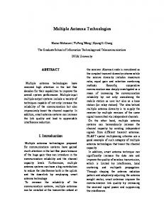
Fig. 1.
Multicast rates for n = 4 and increasing # of users
of the point-to-point capacities: � � C0 (H) ≤ log 1 + P · min khi k2 . i=1,...,m
Using the earlier result on the minimum of chi-square random variables,� the upper bound can be approximated by � 1 log 1 + mP1/n ≈ mP1/n , which is O m1/n . The same white method can be used to show that � on the definition of C 1 white C is O m1/n . To analyze TDMA, notice that the lower 1 1 ) ≈ log(1 + m1/n bound in (2) can be approximated as m 1 . Using the fact that the maximum of chi-squared 1+1/n m random variables grows logarithmically, the TDMA upper 1 bound can readily be approximated as m log log m. Note that similar scaling results for C0 and C white are given in [5][4]. Since the number of users is taken to be large while the number of spatial dimensions is fixed, it is not surprising that the scaling of C0 and C white is similar, as one would intuitively expect the optimal covariance to tend towards the identity matrix so that all spatially dispersed users would receive adequate signal power. Note that TDMA does not scale as well as the multicast capacity or the isotropic input rate because the use of an orthogonal strategy results in 1 . a pre-log factor of m Though no order result is given for C bf , the lower bound � 1 in (1) indicates that C bf grows at least as fast as O m2+1/n , which is rather poor. While this lower bound may be overly pessimistic, it is intuitively clear that beamforming will not perform well when m ≫ n because every beamforming direction will likely be nearly orthogonal to at least one user’s channel. The multicast capacity and the rate achieved with a spatially white input are shown in Figure 1 for a 4 antenna transmitter with an increasing number of receivers. The numerical results indicate that both curves go to zero as O(m−1/4 ), and the order term is shown for reference. B. Fixed Users, Increasing Antennas Next we consider the scenario where the number of users m is fixed while the number of transmit antennas n is
8
10
12
14
16
18
20
Transmit Antennas
Fig. 2.
Multicast rates for 5 user system with an increasing # of antennas
taken to infinity. Here the multicast capacity as well as the beamforming and TDMA rates go to infinity at the same rate, but the rate achieved with a spatially white input is bounded. Proposition 2: If m is fixed and n → ∞, capacity metrics grow at the following rates: C0 C white C bf C
tdma
≈ O (log n) ≈ O (1)
≈ O (log n) ≈ O (log n) .
Proof: We first consider C bf and the lower bound in (1). Since m is finite, the effect of the minimum operation over m random variables is negligible because |hi |2 is chi-squared with degrees of freedom going to infinity. Thus, the lower bound in C bf can be approximated as log(1 + mP2 n), which is O(log(n)). By the same argument, the TDMA bounds in (2) 1 log n, which gives the and (3) can both be approximated as m O(log n) growth of TDMA. The multicast capacity C0 is lower bounded by C bf , and thus grows at least as log n. It is easy to see that the multicast capacity does not grow at a rate faster than this because the multicast capacity is upper bounded by the capacity of the channel to any of the receivers, i.e., C0 (H, P ) ≤ log(1 + P khi k2 ), and this upper bound clearly is O(log n). The fact that C white is bounded follows by noting that C white ≤ 2 log(1 + P khni k ), which converges to log(1 + P ) as n → ∞ [12, Section 4.1]. When there are many more antennas than users, even TDMA achieves the optimal scaling of log n because time must only be split between a finite number of users and the capacity within each time slot increases logarithmically with n. Notice that only the isotropic input performs poorly in this scenario, since it is clearly wasteful to transmit power in all spatial directions when users only occupy m dimensions. Figure 2 presents results for a 5 user channel with an increasing number of transmit antennas. From the plot, the logarithmic growth of the multicast capacity and the bounded behavior of the rate achieved with a spatially white input are
apparent. The rate achieved with transmit beamforming is also shown here, and is seen to be extremely close to the multicast capacity. C. Increasing Users and Antennas Finally we consider the scenario where the number of users (m) and base station antennas (n) simultaneously increase while maintaining a linear constant β = m n > 0, which is commonly referred to as the loading factor in CDMA literature. We first present a lemma showing that the per user SNR is bounded in the large system limit. Lemma 1: The per user received SNR is upper bounded as: p max min h†i Σhi ≤ P · (1 + β)2 , Σ
i=1,...,m
in the large system limit.
Proof: We can clearly upper bound the minimum received SNR by the average received SNR, which gives: max Σ
min h†i Σhi
i=1,...,m
≤ =
m X
m
= =
X 1 hi h†i max Tr Σ m Σ i=1 � 1 max Tr ΣHHH m Σ
!
where H = [h1 h2 · · · hm ] and the maximum operations are over Σ ≥ 0 satisfying Tr(Σ) ≤ 1. It is straightforward to see that the solution to the final maximization is in fact the maximum eigenvalue of the matrix HHH . Furthermore, a fundamental result in random matrix theory states that [13]: p 1 a.s. λmax (HHH ) → (1 + β)2 , m A direct result of this lemma is that the multicast capacity C0 is bounded as the number of users and antennas are taken to infinity at a fixed ratio. Proposition 3: If n and m both tend to infinity at the ratio β= m n > 0, then E(C0 ) ≈ E(C white ) ≈
� khk2 −1 1 − t n 1 , ≤ 2n(1 − t)2 where the last step follows from Chebychev inequality and the 2 fact that khk has mean 1 and variance 1/2n. Combining the n above to bounds we obtain �m � � � β 1 khi k2 − → e 2(1−t)2 , ≥t ≥ 1− P min 2 i=1,...,m n 2n(1 − t) which is clearly positive. Now we can lower bound the expected rate as follows: � � khi k2 ≥ t log (1 + tP ) E(C white (H, P )) ≥ P min i=1,...,m n P
�
2)
→ e
− yVar(|u| (1−t)2
log (1 + tP ) > 0.
Furthermore, Lemma 1 implies that C0 is bounded by a constant: � p � C0 ≤ 1 + P (1 + β)2 .
1 h† Σhi max m Σ i=1 i m X 1 Tr(Σhi h†i ) max m Σ i=1
Since t < 1, we have � � khk2