tunnel. Phalen's maneuver also decreases the space in the carpal tunnel, but is
not very sensitive for detecting CTS. Causes of CTS are variable (congenital ...
Chapter 2
Carpal Tunnel Syndrome, Electroneurography, Electromyography, and Statistics
After reading this chapter you should: • Know what basic techniques are employed in electroneurography • Know what basic techniques are employed in electromyography • Know how electroneurography and electromyography can help diagnose neuromuscular disorders and distinguish neuropathies and myopathies in particular • Understand why normal values are important in clinical practice • Be able to describe the statistical considerations that are important for obtaining normal values • Be able to describe the distribution of a value in a sample by a few statistics
2.1
Patient Cases
Patient 1 For several years, a female 33-year-old patient suffers from numbness and tingling in her right arm and hand, in particular in her index and middle finger. Opening jars has become more difficult, suggesting that the force in her right hand has decreased. Her complaints do not increase when she drives a car or rides a bicycle, nor are the complaints alleviated when she shakes her hand. At night, she incidentally wakes up because of numbness in her fingers. During daytime, the pain in her arm is most prominent. It is already known that she does not suffer from rheumatoid arthritis. The neurological examination does not indicate atrophy of the hand muscles, nor is the force of the abductor pollicis brevis muscle decreased. Her right grasping force is slightly less than normal (MRC 4). The somatosensory function of her hand and fingers is normal. Tapping of the nerves at the wrist does not elicit tingling in the fingers (negative Tinel’s sign), nor does compression of the median nerve in the carpal tunnel by flexion of the wrists (negative Phalen’s maneuver). N. Maurits, From Neurology to Methodology and Back: An Introduction to Clinical Neuroengineering, DOI 10.1007/978-1-4614-1132-1_2, # Springer Science+Business Media, LLC 2012
3
4
2 Carpal Tunnel Syndrome, Electroneurography. . .
Patient 2 A male 61-year-old patient suffers from tingling, numbness, and occasional pain in the thumb, index finger, and middle finger of both hands. His complaints deteriorate at night causing him to wake up sometimes. The numbness and tingling sensations are always present; the patient does not report any movements that improve or deteriorate the complaints. The neurological examination reveals atrophy of the abductor pollicis brevis muscle in both hands, with preserved force (MRC 5). In both hands, the three affected fingers are hypesthetic. Both Tinel’s sign and Phalen’s maneuver are negative.
2.2
Electroneurography: Assessing Nerve Function
The complaints that patients 1 and 2 suffer from are typical for carpal tunnel syndrome (CTS), a group of symptoms caused by compression of the median nerve in the carpal tunnel. The median nerve is a mixed nerve, containing both motor and sensory nerve fibers. Thus, when the nerve is damaged due to compression, this can lead to both motor (muscle weakness and atrophy) and sensory problems (numbness, tingling sensations). The location of the complaints is directly related to the motor and sensory innervation of the median nerve distal to the site of compression, i.e., the motor problems will occur in the thenar muscles whereas the sensory problems will occur in the thumb, index, and middle finger and the radial side of the ring finger. The motor problems mostly do not occur until a later stage of CTS. Different body positions at night can cause an increase in complaints, whereas shaking of the hand can alleviate them, by decreasing or increasing the available space in the carpal tunnel. Phalen’s maneuver also decreases the space in the carpal tunnel, but is not very sensitive for detecting CTS. Causes of CTS are variable (congenital narrow carpal tunnel, hormonal (pregnancy), trauma, rheumatoid arthritis) and cannot always be identified in an individual patient. The test that is most sensitive for diagnosing CTS involves sensory nerve conduction velocity assessment.
2.2.1
Nerve Physiology and Investigation
Nerves consist of several nerve fibers (axons) that are oriented in parallel. When the nerves are myelinated, a fatty myelin sheath covers the axon. This myelin sheath has insulating properties, enabling faster signaling along the nerve. When a motor nerve fiber is stimulated, it will conduct the locally elicited action potential along its membrane via the neuromuscular junction to the motor end plate of the muscle where it will cause muscle fibers to contract. Sensory nerve fibers conduct the action potential to other sensory fibers in the central nervous system, enabling sensations, or to motor neurons, evoking reflexes. To assess the speed of nerve
2.2 Electroneurography: Assessing Nerve Function
5
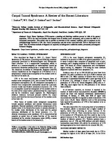
Fig. 2.1 For stimulation at the wrist A indicates antidromic conduction in sensory nerve fibers, B orthodromic conduction in motor nerve fibers, and C orthodromic conduction for sensory nerve fibers and antidromic conduction for motor nerve fibers. Circles and strips indicate stimulation (at the wrist) and recording electrodes, where the dark electrodes are the so-called active electrodes. Distances between active electrodes determine latencies and velocities
signaling (conduction velocity) or the number of normally functioning fibers in a nerve, electroneurography can be used. To investigate nerve conduction velocity, the nerve is stimulated and the time it takes for the evoked potential to arrive at another point along the nerve’s trajectory is recorded. Usually, electrical stimulation is used, because it can be well quantified and all nerve fibers can be stimulated at virtually the same moment. The artificial stimulation typically takes place somewhere along the nerve, thereby evoking a traveling potential in two directions: the natural direction (orthodromic conduction) and the opposite direction (antidromic conduction) (see Fig. 2.1). Stimulation can be performed with needle or surface electrodes; the latter can only be used for superficially located nerves. Both surface and needle electrodes can be used to record the evoked potential at a location distant from the stimulation site. By stimulating a mixed nerve, both motor and sensory functioning can be evaluated.
2.2.1.1
Motor Nerve Functioning
Electrical stimulation of a motor nerve evokes orthodromic action potentials that activate the neuromuscular junction and, secondarily, cause muscle fibers to contract. The sum of all evoked single fiber action potentials (SFAPs) – the compound muscle action potential (CMAP) – can be recorded from the skin using surface electrodes. When evaluating the CMAP, it is essential that the stimulation is strong enough to activate all muscle fibers (supramaximal stimulation). If the CMAP amplitude is maximal, it can be concluded that stimulation was supramaximal. The time between stimulation and CMAP onset is the motor latency. Because latency is determined by CMAP onset (and not by, e.g., its peak), the fastest conducting nerve fibers determine its value. Note that the latency is not solely determined by the nerve conduction velocity; it also includes the time taken to cross
6
2 Carpal Tunnel Syndrome, Electroneurography. . .
Fig. 2.2 CMAPs are derived from surface EMG recorded over the thenar muscle (3) by distal (1) and proximal stimulation (2), generating the distal and proximal motor latencies (DML and PML), which allow to derive motor nerve conduction velocity
the neuromuscular junction and to travel from the junction to the electrode overlying the muscle belly. Therefore, nerve conduction velocity is determined by stimulating at two different (distal and proximal) locations along the nerve while recording from the same position (see Fig. 2.2). Question 2.1 How can the distal and proximal latencies be used to derive the conduction velocity of the nerve segment between the two stimulation positions? Remember that velocity is calculated as (distance traveled)/(time traveled). For motor nerve conduction velocity studies of the main nerves in the arm (median and ulnar nerve), the distal stimulation site is usually at the wrist while the proximal stimulation point is at the elbow. For the main nerves in the leg (tibial and peroneal nerve), the distal stimulation site is usually at the ankle and the proximal stimulation site at the knee. Depending on the clinical question, more proximal stimulation sites may also be used. The CMAP amplitude, measured from top to baseline or from top to top, gives information about the number of (supramaximally) activated muscle fibers. By comparing the CMAPs between distal and proximal stimulation and between both sides of the body, important diagnostic information can be derived. In a normally functioning nerve, both distal and proximal stimulation should stimulate all axons going to the muscle that the CMAP is recorded from. Because the difference in arrival time at the recording site of action potentials in the fastest conducting fibers
2.2 Electroneurography: Assessing Nerve Function
7
Fig. 2.3 Schematic overview of a nerve consisting of five myelinated axons. (a) Normal nerve, with intact myelin sheath. The CMAP morphology is similar between proximal and distal stimulation. (b) Segmental demyelination: the myelin sheath has been damaged multifocally. The distal CMAP is normal, but the proximal CMAP has lower amplitude and becomes broader, because the conduction velocity varies strongly between axons. (c) Axonal degeneration: several axons have completely disappeared. Functioning of the remaining axons has been preserved resulting in normal conduction velocities but lower amplitude CMAPs
compared to those in the slowest conducting fibers will be larger for proximal stimulation, leading to more temporal dispersion, the amplitude of the proximally stimulated CMAP will be slightly lower and the peak slightly broader. In normal motor nerves, these differences are minimal however. There are three pathological mechanisms that can underlie disturbed nerve conduction: axonal degeneration, segmental demyelination, and conduction block (see Fig. 2.3).
8
2 Carpal Tunnel Syndrome, Electroneurography. . .
Axonal degeneration entails the functional loss of some motor axons, typically over the entire trajectory of the nerve, inducing a decreased CMAP amplitude for proximal as well as distal supramaximal stimulation. Depending on which axons are affected, the latency may be normal or increased. Segmental demyelination causes decreased nerve conduction velocity in the part of the axon that is affected. If all axons in a nerve are affected, nerve conduction velocity can become severely diminished. Since the axons themselves are still intact, the CMAP amplitude should be preserved. However, the CMAP amplitude can be decreased (and the CMAP can have a broader peak) because of increased temporal dispersion of nerve action potentials along the different axons. Finally, conduction block involves complete cessation of conduction, with an intact axon. If the conduction block is located between the proximal and distal stimulation points, the proximal CMAP amplitude will be decreased whereas the distal CMAP amplitude will be normal. F-Responses When a peripheral (motor) nerve is stimulated supramaximally, potentials are conducted orthodromically evoking a muscle response (M-response). At the same time, potentials are also conducted antidromically and arrive at the motor neurons in the anterior horn of the spinal cord. Some of these motor neurons are then depolarized and send potentials back through the motor nerve fibers (orthodromically again), yielding the later F-response. It is named after its first recording in a foot muscle. The number and type of motor neurons that depolarize differs from stimulus to stimulus, changing the latency, amplitude, and shape of the F-response. Often, the minimum F-response latency is recorded, which reflects only the fastest motor axon contributing to the F-response. This value can be normal in pathology, however. Therefore, the dispersion in F-response latency is more helpful in diagnosing disorders of the proximal segments of motor nerves. Note that F-latencies depend on height and it is thus better to interpret F conduction velocities rather than latencies. For longitudinal recordings, latencies are very useful, however.
2.2.1.2
Sensory Nerve Functioning
As mentioned before, both sensory and motor nerve functioning can be assessed by stimulating a mixed nerve. When a peripheral nerve is damaged, often both sensory and motor functioning are affected; although when damage to the nerve is still limited, there may be sensory dysfunction while motor functioning is still normal. Assessing sensory nerve function is also important for those diseases in which sensory nerves are selectively involved. When a sensory nerve is or sensory nerve fibers are stimulated by surface electrodes, the (compound) sensory nerve action potential (SNAP) can be obtained from another location along the nerve, by surface or needle electrodes. Both orthodromic and antidromic methods are in use. The sensory nerve conduction velocity can be determined similar to the motor nerve conduction velocity, i.e., by stimulating distally and proximally along the nerve, recording from a more distal
2.2 Electroneurography: Assessing Nerve Function
9
site along the nerve, and comparing the distal and proximal sensory latencies (DSL and PSL). A difference with motor conduction velocity is that the DSL can also be directly used to derive the sensory nerve conduction velocity in that trajectory, since the SNAP is directly recorded from the nerve, in contrast to the CMAP which is recorded from the muscle. Question 2.2 What distance needs to be determined to derive the sensory nerve conduction velocity based on the DSL?
2.2.1.3
Factors Influencing Nerve Conduction
As all things move slower when it is cold, it is not surprising that nerve conduction velocity is reduced at colder temperatures. At the same time SNAP amplitudes are increased at colder temperatures. These temperature effects mainly result from slower functioning of the sodium and potassium channels in the nerve cell membrane. The changes in nerve conduction with temperature have two important practical consequences. First of all, any reported (motor or sensory) nerve conduction velocity should include the (skin) temperature at the recording site (and preferably also at the stimulation site). Otherwise, a second measurement in the same subject cannot be interpreted well. Second, it is even better to always record nerve conduction velocities at the same (skin) temperature, so that values can be compared to normal values or to values obtained at another occasion in the same patient, without having to resort to conversion formulas. This can be achieved in practice by warming up the patient with warm blankets, infrared lamps, or warm water baths until the required temperature is reached (preferably 32� C at the skin). Another factor influencing nerve conduction is age, which is especially important for recordings in young children. After the age of 3–5 years, nerve conduction velocities have typically increased to normal adult values. The increase in conduction velocity with age in young children largely results from an increase in nerve fiber diameter (the thicker the nerve fiber the faster it conducts) and from increased myelination. In older adults nerve conduction velocity gradually decreases again. Kimura (2001) has reported normal values for different nerves and age groups.
2.2.2
Diagnosing Carpal Tunnel Syndrome
To understand the logic of the electroneurographic investigation in CTS, it is important to know the trajectories of the main nerves in the lower arm and hand with respect to the carpal tunnel (see Fig. 2.4) on the side of the palm of the hand. The median nerve passes through the carpal tunnel whereas the other two nerves do not. Furthermore, the radial side of the ring finger is innervated by the median
10
2 Carpal Tunnel Syndrome, Electroneurography. . .
Fig. 2.4 Schematic overview of the trajectories of the radial (dashed), median (drawn), and ulnar (dotted) nerves and some of their branches in the wrist and hand. See text for explanation of the numbers
nerve, while its ulnar side is innervated by the ulnar nerve. Similarly, the thumb is innervated by the median nerve on the side of the palm of the hand and by the radial nerve on the other side. The diagnosis of CTS relies on two investigations: the motor conduction of the median nerve and the sensory conduction of the median nerve. If the median nerve is compressed in the carpal tunnel, it is expected that conduction velocity is decreased, causing the DML to increase, due to focal demyelination. The conduction velocity itself cannot be determined for the most distal part of the motor nerve because of the unknown delay at the neuromuscular junction, only the DML can be reported. To be able to directly compare the DML in a patient to values obtained in healthy subjects, it is important that the same distance (usually 7 cm) between stimulation and recording sites is used. Furthermore, in slight cases of CTS the motor conduction velocity in the lower arm will still be normal, but when CTS is severe the median nerve may demyelinate causing a decreased motor conduction velocity. In addition, axonal damage may occur. To determine if the sensory nerve conduction velocity of the median nerve is affected, SNAPs are recorded from the fingers that are innervated by the median nerve and one of the other nerves that do not pass through the carpal tunnel, i.e., from the thumb (I in Fig. 2.4) for the radial nerve and from the ring finger (IV in Fig. 2.4) for the ulnar nerve. By stimulating each of the nerves at the wrist proximal from the carpal tunnel (1, 2, and 3 for the radial, median and ulnar nerves and CT for the carpal tunnel in Fig. 2.4) at the same distance from the recording electrode, SNAP latencies can be compared between the possibly trapped median nerve and the other nerves. If the latency difference is larger than 0.4 ms, conduction of the sensory median nerve fibers is disturbed, which is assumed to be a sign of CTS. In principle, to
2.3 Electromyography: Assessing Muscle Function
11
exclude other causes of the CTS symptoms, it may be necessary to additionally investigate motor conduction of the ulnar nerve, or the function of one of the muscles innervated by the ulnar nerve by (needle) electromyography.
2.3
Electromyography: Assessing Muscle Function
Needle electrodes can also be used to assess muscle fiber functioning by recording their electrical activity from a close distance (needle electromyography). When muscle fibers are activated at the motor end plate, action potentials start to propagate in two directions, similar to what happens in activated nerve fibers. These single fiber action potentials (SFAPs) induce contraction of the muscle fiber by a so-called electromechanical coupling mechanism. Electromyography only allows studying the electrical and not the mechanical phenomena of muscle contraction. A needle electrode, although very thin, is too large to record individual SFAPs, except in pathological circumstances in which muscle fibers can discharge spontaneously and independently. A needle electrode will typically record the activity of multiple muscle fibers belonging to the same or multiple activated motor units. During needle EMG the muscle is investigated at rest, during weak contraction to evaluate individual action potentials, and during strong contraction to evaluate the full contraction pattern. For a more detailed account of electromyographic investigations please see the references. Here, only some basic concepts are discussed. An EMG needle has a very small field of view, allowing picking up the activity of a limited number of muscle fibers directly and of more fibers at a larger distance, depending on needle type. All SFAPs that develop within the field of view of the electrode when a muscle is contracted add up to the motor unit potential (MUP) that is actually recorded. The SFAPs at a larger distance contribute only partially to the MUP, because of volume conduction effects that act as a low-pass filter (see Sect. 4.3.4). The number of fibers within the field of view of the electrode, the distance of the active fibers to the electrode, and the timing between the SFAPs all contribute to the shape of the MUP. Normally, the timing of SFAPs contributing to the MUP is highly synchronized, invoking only 3–4 peaks in the MUP. An MUP that has more than four peaks (phases) is called polyphasic. The presence of too many polyphasic MUPs can indicate neuropathies (mostly large strongly polyphasic MUPs) or myopathies (small polyphasic MUPs). Note that these characteristics are different for recent neuropathies and long-existing myopathies. Besides MUP evaluation, another important aspect of needle electromyography is the assessment of muscle contraction patterns (see Fig. 2.5). During weak contraction only a few motor units should be activated, resulting in a pattern with only a couple of separately distinguishable MUPs (single pattern). When the contraction level is increased, more and faster firing motor units should be recruited, resulting in a full contraction pattern in which the individual MUPs can no longer be distinguished (interference pattern). The maximum amplitude in
12
2 Carpal Tunnel Syndrome, Electroneurography. . .
Fig. 2.5 Examples of contraction patterns during (a) weak (single pattern with two identifiable motor units), (b) moderate (mixed pattern), and (c) strong (interference pattern) contraction. The duration is 2 s for every top signal and 200 ms for every bottom signal. Signals were obtained from needle EMG of the m. extensor digitorum communis in the lower arm
the interference pattern may be increased in case of a chronic neuropathy and decreased in case of a myopathy, due to the presence or absence of large MUPs. In between the single and interference pattern a mixed pattern exists, which may occur when a healthy muscle cannot be contracted optimally due to pain or fear, or as a result of pathology. A (single or mixed) contraction pattern can be analyzed automatically to extract the different involved motor units. Normally, during rest, there should be no muscle activity. However, needle insertion or repositioning can result in activity due to mechanical stimulation of the muscle fibers. In addition, when the needle is inserted close to the motor endplate zone, spontaneous miniature endplate potentials, not resulting in action potential propagation, may be recorded. Other potentials occurring during rest, such as fibrillations and positive sharp waves, indicate pathology. Fibrillations have two or three phases, last 1–5 ms and start with a positive phase. They are discharges of individual muscle fibers and indicate changes
2.4 Diagnostic Measures: What Is (Ab)normal?
13
in membrane properties usually due to axonal degeneration in the nerve innervating the muscle fiber (denervation). Positive sharp waves occur under similar circumstances as fibrillations, start with a short positive phase followed by a long negative phase and last approximately 10 ms. Spontaneous motor nerve discharges can also lead to MUPs during rest. Examples are fasciculations and spontaneous rhythmic MUPs. Fasciculations occur spontaneously and completely irregularly and can be observed through the skin as muscle twitches when they are superficially located. They can be both benign and pathological. Spontaneous rhythmic MUPs are purely rhythmical (in contrast to contraction patterns due to volitional contraction) at 3–9 Hz. They can be seen in nerve compression syndromes such as CTS. The electromyogram can also be recorded using surface electrodes, as for recording of the CMAP. Surface recordings prohibit the evaluation of individual MUPs, however.
2.4
Diagnostic Measures: What Is (Ab)normal?
As referred to in the previous sections, for reliable and consistent interpretation of electroneurographical and electromyographical measures (or any other measure obtained in a patient for that matter), it must be possible to determine if a patient’s value falls within the normal range or not. This normal range is also referred to as reference range, reference values, or normal values.
2.4.1
Sampling the Population
To obtain normal values for a certain laboratory test, a representative sample of the general population needs to be taken and the test value must be obtained in this population under the same circumstances as will be used clinically. This implies that normal values should ideally be obtained for each laboratory and each machine again, although some test values differ so little between laboratories that normal values can be adopted from another laboratory. A representative sample of the population must have the same characteristics as the group of patients that they will be compared with, in the same proportion. In addition the sample must be chosen randomly to avoid bias. When the sample is large enough and selectively chosen, it is usually representative. If it is known beforehand that certain parameters that describe population characteristics have a great influence on the test value (e.g., age, sex, ethnicity), they can be taken into account for the composition of the population sample. In practice 30–40 subjects may be measured to obtain normal values, or ten per subcategory if a distinction is made on the basis of, e.g., age or weight. However, the exact number of subjects needed to represent all possible outcomes of the test value in the normal population depends strongly on the characteristics of the test value’s distribution and of course, the larger the sample the better the estimate.
2 Carpal Tunnel Syndrome, Electroneurography. . .
14
Fig. 2.6 Example of a normal distribution
2.4.2
Normal Distributions
For test values that depend on many independent variables (such as for most medical tests), it is often the case that the histogram of values obtained in a large population of different subjects will have a characteristic bell-shaped distribution known as the Gaussian or normal distribution (see Fig. 2.6). When a test value in a population sample follows a normal distribution, it is usually assumed that the test value will follow the same distribution in the entire population. The beauty of a normal distribution is that its graph can be completely described by two parameters, the mean m and the standard deviation s, as follows: �ðx�mÞ2 1 f ðxÞ ¼ pffiffiffiffiffiffiffiffiffiffi e 2s2 2ps2
(2.1)
The mean m is the center of the distribution and this value is mostly found in the population. When s is small, the distribution is closely centered around the mean, whereas when s is large, the distribution is very widespread. In the standard normal distribution, m ¼ 0 and s ¼ 1. Furthermore, independent of the exact values for m and s, exactly 95% of the values in the distribution lies between m � 1:96s and m þ 1:96s and 99% of the values lies between m � 2:58s and m þ 2:58s. In practice the two parameters m and s are estimated from a population sample with size N and values xi as follows: x� ¼
N 1 X xi N i¼1
(2.2)
2.4 Diagnostic Measures: What Is (Ab)normal?
s¼
vffiffiffiffiffiffiffiffiffiffiffiffiffiffiffiffiffiffiffiffiffiffi uN uP u ðxi � x�Þ ti¼1 N�1
15
(2.3)
Here, the estimates for m and s are indicated by x� and s. By replacing m and s by x� and s, it can be seen that 95% of the values in the population sample lies between x� � 1:96s and x� þ 1:96s, if it is normally distributed. This interval can be used as an estimate of the reference interval for a particular laboratory test that can then be used for diagnostic purposes. However, instead of the factor 1.96, the factor 2.58 may be used (99% of the values) or, for ease of use, the factors 2.5 and 3 are also common. In these cases, values are thus said to be abnormal if they are higher (or lower) than the mean + (or �) 2.5 or 3 standard deviations. The higher this factor the fewer false positives a laboratory test will find in pathological cases (higher sensitivity). If it is more important to have a high specificity (fewer false negatives), this factor may be chosen lower.
2.4.3
Descriptive Statistics
The mean and standard deviation as calculated in (2.2) and (2.3) are examples of descriptive statistics. Formally (and rather abstractly), a statistic is a single measure of some aspect of a sample, which can be calculated by applying some formula on the individual values in a sample (or dataset). In other words: a statistic summarizes an important property of a dataset in a single number. Statistics for datasets can be roughly divided into two categories: measures of location and measures of variability. Measures of Location The most well known and often used measure of location is the (arithmetic) mean as defined in (2.2). The advantage of the mean is that it uses all values in a dataset and can help to characterize the distribution of the data as in the normal distribution. The main disadvantage of the mean is that it is very vulnerable to outliers: single values that, when excluded, have a large influence on the results. Outliers cannot be simply removed from the dataset, unless there are very good reasons to do so, such as known measurement errors or a value that actually belongs to a different population than the rest of the sample. An alternative measure of location, that is less sensitive to outliers, is the median. The median is the middle value (or the mean of the middle two values if there is an even number of values in the sample) if all values in the sample are ordered in size. The disadvantage of the median of course is that it does not use all values in the sample. A third measure of location is the mode, the most frequently occurring value in the sample. It is not used very much, except for measures such as modal income. In case of a normal distribution, mean, median, and mode have the same value. Other measures of location are quartiles (lower, median, and upper) and percentiles. The quartiles are the values that divide the data into four equal parts, each cutting off another 25% of the data values. The quartiles can be
2 Carpal Tunnel Syndrome, Electroneurography. . .
16
found by ordering the values again and determining the value that has 25% of the other values below it and 75% of the other values above it for the first quartile, etc. The median is equal to the second quartile.
Question 2.3 What are the mean, median, mode, and first quartile for the following dataset: {1, 3, 2, 4, 5, 2, 2, 6, 1, 2, 3, 2, 4, 1, 2, 6, 4, 5, 3, 2, 2, 3, 4, 5, 4, 2, 3, 1}?
Percentiles are the values that have a certain percentage of the values below them when ordered. The tenth percentile thus has 10% of the values in the dataset below it and 90% of the values above it. The first or lower quartile is thus equal to the 25th percentile, the second quartile (median) to the 50th percentile, and the third or upper quartile equals the 75th percentile. Measures of Variability The standard deviation (SD) as calculated in (2.3) is a measure of variability. Its square is the variance. From (2.3) it can be seen that s would be zero when all xi would be the same, i.e., when there would be no variability in the sample. On the other hand, when the xi are all very different from the mean x�, s would be very large. As mentioned earlier, about 95% of the values in a normally distributed sample lies within two standard deviations from the mean. When data is not normally distributed, there are more appropriate measures of variability that not automatically assume symmetry of the distribution. The range is defined as the difference between the smallest and largest samples in the value. The interquartile range (IQR) is given as the difference between the first and third quartiles and is less sensitive to outliers than the range.
2.4.4
Correlations
Normal values can only be defined on the basis of a representative sample when it is homogeneous, i.e., when there are no properties on which individual subjects differ and that, when the group would be split on that property, would give different distributions in the subgroups. For example, length depends on age and sex; clothes size depends on weight, age, and sex; and nerve conduction velocities depend on temperature. Thus, normal values for length cannot be derived from a sample that contains widely different ages or both men and women, but subcategories should be made for each of these variables. To determine if normal values should be given for subcategories, it should be determined whether the value under consideration is associated with (depends on) the value of another independent variable. This can be achieved by correlation analysis when the two variables under
2.4 Diagnostic Measures: What Is (Ab)normal?
17
consideration are both continuous (vary smoothly). The correlation coefficient is a statistic that summarizes the strength of the relationship between two variables and can vary between �1 (strong negative correlation) and +1 (strong positive correlation). A correlation coefficient of 0 indicates that there is no correlation. Its calculation is explained in Box 2.1.
Box 2.1 The Correlation Coefficient When a linear relationship between two variables x and y is expected, Pearson’s correlation coefficient can be calculated for a sample of N measurements of these variables, given as xi and yi , as follows: N P
1 rxy ¼ N�1
ðxi � x�Þðyi � y�Þ
i¼1
sx sy
(1)
Here x� and y� are the sample means and sx and sy the sample standard deviations of x and y as calculated in (2.2) and (2.3), respectively. Pearson’s correlation coefficient is not sensitive to nonlinear relationships. In that case a rank correlation coefficient (Kendall’s or Spearman’s) can be calculated, which measures the extent to which one variable increases/ decreases as the other variable increases/decreases, without assuming that this increase is explained by a linear relationship.
Note that Pearson’s correlation coefficient only indicates the presence of a linear relationship between variables. If there is a strong but nonlinear relationship between variables, Pearson’s correlation coefficient can be close to zero. Examples are given in Fig. 2.7. The correlation coefficient is closer to 0 when the data is noisier, positive for positive slopes, and negative for negative slopes of the linear relation. Yet, the value of the correlation coefficient does not reveal the slope of the linear relation itself. A common misconception about correlation is that a high value necessarily reflects a causal relationship between variables, although it can be indicative of one. Other approaches are needed to establish a causal relationship. A correlation analysis can indicate whether normal values need to be given for subcategories. For example, in one of our own studies (Maurits et al. 2004), we determined normal values for muscle ultrasound parameters in children. We first calculated correlations between muscle ultrasound parameters and all independent variables (length, weight, BMI, and age) for each gender (48 boys and 57 girls between the ages of 45 and 156 months were included). Although normal values in children are often given per age group, we first determined which of the variables that correlated with the muscle ultrasound parameters would predict them most strongly by linear regression analysis (see references for details). More sensitive
18
2 Carpal Tunnel Syndrome, Electroneurography. . .
Fig. 2.7 Examples of scatter plots of two variables x and y indicating (a) strong positive correlation, (b) no correlation, and (c) weak negative correlation. An example where the correlation coefficient is inappropriate to describe the relationship between x and y is given in (d) for a quadratic relationship and in (e) for an outlier
parameters for clinical practice are obtained if classification is performed according to the most predictive variable. The results showed that normal values for subcutaneous tissue thicknesses should be given as a function of BMI, for muscle thicknesses as a function of weight and all other muscle parameters actually did not depend on length, weight, BMI, or age. Note that none of the muscle parameters were eventually given as a function of age.
2.4 Diagnostic Measures: What Is (Ab)normal?
2.4.5
19
Tips and Tricks When Using Descriptive Statistics
Although descriptive statistics and correlations are not difficult to calculate, there are some practical guidelines that should be considered when using these summarizing measures.
2.4.5.1
Normality
In the previous sections, it was indicated that it is important to know whether the distribution of a value in a sample is normal, to determine which descriptive statistics can be used to describe the distribution. There are different ways to assess normality of a distribution. The simplest is to plot a histogram of the values in the distribution. If its shape is Gaussian (looks like a symmetric bell; see Fig. 2.6), it is likely that the distribution is normal. An important aspect of normal distributions is that they are symmetric around the mean. If the distribution is not symmetric, but has a longer tail to the left (lower values), it is left skewed; if the longer tail is to the right (higher values), it is right skewed (see Fig. 2.8). If a distribution is skewed, the median and IQR are more appropriate summary measures than the mean and SD which are sensitive to the skewness. A measure of skewness is the third moment around the mean: vffiffiffiffiffiffiffiffiffiffiffiffiffiffiffiffiffiffiffiffiffiffiffi uN uP u ðxi � x�Þ3 ti¼1
(2.4)
s3
A simpler expression for skewness exploits the fact that in a normal distribution, the mean and median are close: �
Mean � Median 3 s
� (2.5)
Question 2.4 Will skewness according to (2.5) be positive or negative for right-skewed distributions?
In some cases, appropriate transformations of the data can make non-normal distributions normal (see Box 2.2). Other ways to assess normality of distributions is by exploring the so-called Q–Q plots. A Q–Q plot (where Q stands for quantile) allows comparing two distributions (e.g., a theoretical normal distribution with the distribution in a sample) by plotting
20
2 Carpal Tunnel Syndrome, Electroneurography. . .
Fig. 2.8 Examples of (a) left-skewed and (b) right-skewed distributions
their quantiles against each other. If the pattern of points in the plot resembles a straight line, the distributions are highly similar. Examples of quantiles are the 2-quantile (the median), 4-quantiles (the quartiles), and 100-quantiles (the percentiles). Finally, some statistical tests can be used to assess normality of a distribution (e.g., the Shapiro–Wilk or Kolmogorov–Smirnov test). When the distribution of the values for a laboratory test in a population sample is not normal, and cannot be made normal by a transformation, defining normal values on the basis of the SD is not appropriate. Before resorting to other methods, it is first important to check whether the distribution is not normal because it is bi- or multimodal, i.e., has multiple peaks. This may indicate that two or more different populations (e.g., males and females) underlie the distribution and the total sample
2.4 Diagnostic Measures: What Is (Ab)normal?
Box 2.2 Normalizing Skewed Distributions To normalize a right-skewed distribution, larger values in the distribution must be decreased more than low values in the distribution. To accomplish this, we need a transformation that has relatively low output for high input values and relatively high output for low input values. A suitable transformation to achieve this is the (natural or 10-base) logarithm (Fig. 2.9a). Similarly, to normalize a left-skewed distribution, we need a transformation that has relatively high output for high input values and relatively low output for low input values. A suitable transformation for left-skewed distributions is a quadratic function (Fig. 2.9b).
Fig. 2.9 Example of (a) logarithmic function y ¼ ln x and (b) quadratic function y ¼ x2
21
22
2 Carpal Tunnel Syndrome, Electroneurography. . .
should then first be split. If this is not the case, percentiles (see Sect. 2.4.3) may be used to define normal values. If low values on the laboratory test are abnormal, the 1st, 5th, or 10th percentile may be used as a cut-off value; if high values on the laboratory test are abnormal, the 90th, 95th, or 99th percentile may be used. Finally, the most extreme value seen in healthy subjects may also be used as a limit for the normal range.
2.4.5.2
Plotting Before Calculating
There are at least two reasons for plotting data before calculating descriptive statistics or correlations. As mentioned in Sect. 2.4.3, some descriptive statistics are sensitive to outliers. Outliers are most easily detected by plotting the data in an appropriate manner (in a dot plot, histogram, or boxplot; see Fig. 2.10). As indicated in Sect. 2.4.4, correlations between two variables can only be calculated if a linear relationship is expected between the two. To investigate if a nonlinear relationship is more likely, the two variables can first be plotted against each other in a scatter plot (see Fig. 2.7). Thus, plotting before calculating prohibits making some elementary mistakes in calculating statistics.
2.4.5.3
Reliability of Sample Statistics
Although it was mentioned earlier (Sect. 2.4.1) that a sample that is large enough and selectively chosen, is usually representative for the entire population, there is still a need to know how reliable sample statistics are. In other words: if we would take another representative sample of the population, how likely is it that we would find a similar estimate for the sample statistic? The precision with which a mean is estimated can be inferred from the standard deviation of the mean, more commonly referred to as the standard error of the mean (SE). It is calculated by dividing the standard deviation of the sample by the square root of the number of subjects making up the sample: s SE ¼ pffiffiffiffi N
(2.6)
This definition formally confirms the more intuitive notion that the sample mean becomes more reliable (i.e., SE becomes smaller) when the number of subjects in the sample is larger. To be clear, the difference between s and SE is that s provides a measure of the variability between individuals related to the laboratory test value, whereas SE provides a measure of the variability in the mean, derived from the individual values, from sample to sample. Note that because SE is always (much) smaller than s, some authors display SE in figures instead of s. This is a very deceptive practice, because it suggests less variability in individual test values than are actually present in the sample.
2.4 Diagnostic Measures: What Is (Ab)normal?
23
Fig. 2.10 Examples of (a) dot plot, (b) histogram, and (c) boxplot
2.4.5.4
Statistical Group Differences and Individual Patients
Normal values are employed to distinguish patients from healthy subjects. In literature many studies can be found that compare groups of patients to groups of healthy controls finding statistically significant differences between groups. It is important to realize that this does not imply that the measure under investigation is necessarily a sensitive measure to distinguish one individual patient from healthy subjects. For example, even when there is a lot of overlap in the distributions of the test value for patients and healthy subjects, a statistically significant difference may still be present (when the groups are large enough). Yet, in that case, an individual patient is highly likely to be within normal range and cannot be distinguished from healthy subjects. Better measures to predict the applicability of a measure for diagnostic purposes are sensitivity and specificity. Sensitivity is the percentage of patients that is correctly identified as being patients and specificity is the percentage of healthy subjects that is correctly identified as being healthy.
24
2 Carpal Tunnel Syndrome, Electroneurography. . .
Fig. 2.11 CMAPs as obtained from the abductor pollicis brevis muscle after (a) left and (b) right distal (top) and proximal (bottom) stimulation of the median nerve in patient 1
2.5
Electroneurography in Individual Patients
Both patients 1 and 2 were investigated after warming up their lower arms in a warm water bath. Subsequently, motor and sensory conduction velocities were determined through electroneurography. Normal values were the same as those given by Kimura (2001). Deviations from the normal mean are given in SD. Patient 1 The median nerve motor conduction velocity in the lower arm was determined by stimulating at the wrist and elbow and recording from the abductor pollicis brevis muscle. For the left arm, the DML was 2.35 ms (�3.4 SD, i.e., shorter (better) than the mean normal latency) and the PML was 6.05 ms, resulting in a conduction velocity of 65 m/s over a distance of 24.5 cm (+1.4 SD, i.e., faster (better) than the mean normal velocity) over the lower arm. For the right arm, the DML was 2.4 ms (�3.2 SD) and the PML was 6.25 ms, giving a conduction velocity of 64 m/s over a distance of 24 cm (+1.1 SD) over the lower arm. Thus, the median nerve motor conduction velocity was normal in both arms. In Fig. 2.11 the left and right CMAPs resulting from distal and proximal stimulation are shown. In addition, to assess nerve conduction in the most distal part of the median nerve, the DML was compared between the median nerve and the ulnar nerve, by stimulating at the wrist proximal from the carpal tunnel, at the same distance (8 cm) from the recording electrodes over the second lumbrical muscle (innervated by the median nerve) and the second palmar interosseus muscle (innervated by the ulnar nerve). The DML was 2.70/2.75 ms for the left/right median nerve and 2.75/2.80 ms for the left/right ulnar nerve. The differences between the median and ulnar nerve were (far) smaller than 0.5 ms, implicating a normal DML for the median nerve.
2.5 Electroneurography in Individual Patients
25
Fig. 2.12 (a) Left and (b) right SNAPs as obtained from the thumb (first and second trace) and ringfinger (third and fourth trace) after stimulation of the median nerve (first and third trace), the radial nerve (second trace) and the ulnar nerve (fourth trace) in patient 1 Table 2.1 Findings of sensory nerve conduction velocity investigation in patient 1 Latency (ms) Distance (mm) Velocity (m/s) Left Thumb Median nerve 1.85 90 48.6 Radial nerve 1.80 90 50.0 Ringfinger Median nerve 2.35 130 55.3 Ulnar nerve 2.15 130 60.5 Right Thumb Median nerve 1.95 80 41.0 Radial nerve 1.70 80 47.1 Ringfinger Median nerve 2.35 120 51.1 Ulnar nerve 2.20 120 54.5
Finally, sensory nerve conduction velocities were determined by stimulating the nerves at the wrist proximal from the carpal tunnel and recording from the thumb (for a comparison between median nerve and radial nerve conduction velocities) and from the ring finger (for a comparison between median nerve and ulnar nerve conduction velocities) using ring electrodes. The SNAPs are illustrated in Fig. 2.12, and Table 2.1 gives a numerical overview of the findings. In conclusion, motor conduction velocities for the median nerve were normal in both lower arms, as were the DMLs. Sensory conduction velocities were normal as well. Together, motor and sensory conduction studies do not give any indications for CTS in this patient, despite her motor and sensory problems. Her problems (pain and numbness) were finally thought to be of tendomyogenic origin. Patient 2 The investigation proceeded along similar lines in patient 2 as in patient 1. For the left arm, the DML was 8.80 ms (+15.6 SD, i.e., longer (worse) than the mean normal latency) and the PML was 14.20 ms, resulting in a conduction velocity
26
2 Carpal Tunnel Syndrome, Electroneurography. . .
Fig. 2.13 CMAPs as obtained from the abductor pollicis brevis muscle after (a) left and (b) right distal (top) and proximal (bottom) stimulation of the median nerve in patient 2. The proximal stimulation of the right median nerve probably costimulated ulnar nerve fibers, causing the first large positive deflection in the bottom right trace. The second positive deflection is the median nerve CMAP, comparable to the one in the top right trace. Note that the vertical scale differs between the two figures (a) 5 mV per division and (b) 1 mV per division
Fig. 2.14 (a) Left and (b) right SNAPs as obtained from the thumb (first and second trace) and ringfinger (third and fourth trace) after stimulation of the median nerve (first and third trace), the radial nerve (second trace) and the ulnar nerve (fourth trace) in patient 2. Note that the vertical scale is only 20 mV per division
of 44 m/s over a distance of 24 cm (�3.0 SD, i.e., slower (worse) than the mean normal velocity) over the lower arm. For the right arm, the DML was 8.65 ms (+15.2 SD) and the PML was 16.15 ms, giving a conduction velocity of 36 m/s over a distance of 27 cm (�4.9 SD) over the lower arm. Thus, the median nerve motor
2.5 Electroneurography in Individual Patients
27
Table 2.2 Findings of sensory nerve conduction velocity investigation in patient 2 Latency (ms) Distance (mm) Velocity (m/s) Left Thumb Median nerve – 100 – Radial nerve 2.20 100 45.5 Ringfinger Median nerve – 130 – Ulnar nerve 2.40 130 54.2 Right Thumb Median nerve – 100 – Radial nerve 2.40 100 41.7 Ringfinger Median nerve – 140 – Ulnar nerve 2.75 140 50.9
conduction velocity was abnormal in both arms. In Fig. 2.13 the left and right CMAPs resulting from distal and proximal stimulation are shown. When comparing the CMAPs from patient 2 with those in patient 1, it can be clearly seen that the amplitudes are also much lower in patient 2 and the waveform is more dispersed in time, possibly reflecting axonal degeneration and segmental demyelination (see Sect. 2.2.1.1). When stimulating at the wrist proximal from the carpal tunnel, at the same distance (left: 9 and right: 10 cm) from the recording electrodes over the second lumbrical muscle and the second palmar interosseus muscle, the DML was 9.65/7.45 ms for the left/right median nerve and 3.25/3.95 ms for the left/right ulnar nerve. The differences between the median and ulnar nerve were (far) larger than 0.5 ms, implicating a strongly abnormal DML for the median nerve as well. In this patient, F-responses (see Sect. 2.2.1.1) were additionally obtained in the right hand by stimulating the median nerve at the wrist and recording from the abductor pollicis brevis muscle. The F-wave conduction velocity was found to be 47 m/s (�5.3 SD). In this patient, sensory nerve conduction velocities were also obtained: SNAPs are illustrated in Fig. 2.14, and Table 2.2 gives a numerical overview of the findings in patient 2. Note that SNAPs could not be obtained at all when stimulating the median nerve and SNAP amplitudes for the other nerves were normal but low. To summarize, motor conduction velocities were abnormal in both lower arms, DMLs were strongly increased bilaterally, and the DML difference for the median nerve to the lumbrical muscle compared to the ulnar nerve to the interosseus muscle was considerable. CMAP amplitudes were low to very low. The F-response indicated an increased DML, but a surprisingly normal proximal motor conduction velocity. Sensory conduction velocities could not be established for the median nerve in either hand, because SNAPs could not be obtained in the thumb, middle, or ring finger, not even when stimulating at the hand palm. The radial and ulnar nerve had normal sensory conduction. Together,
28
2 Carpal Tunnel Syndrome, Electroneurography. . .
these findings are in accordance with severe CTS in both hands, with considerable axonal degeneration. Because of the severity of his problems, patient 2 was referred to the neurosurgeon for surgery. During this procedure, the transverse carpal ligament that forms the roof of the carpal tunnel will be cut in two, thereby relieving the pressure on the median nerve. If his problems would have been less severe, localized corticosteroid injections could have been given. These injections with anti-inflammatory drugs only temporarily relieve the symptoms of CTS, but this may be sufficient when strategic adaptations to how the hands are used can prevent recurrence of the problems. Although patients 1 and 2 had similar mostly sensory (numbness, tingling, pain) problems, the electroneurographical investigation clearly indicated that CTS was highly unlikely in patient 1 and very likely in patient 2. In this sense, electroneurography can be very helpful in diagnosing neuropathies. Note that for these patients, the clinical tests for CTS (Tinel’s sign and Phalen’s maneuver) were not contributing to the diagnosis.
2.6
Other Applications of Electromyography in Neurology
In Sect. 2.2.1.1, it was shown that surface EMG can be used to assess the CMAP. The CMAP is also recorded in the context of transcranial magnetic stimulation to assess central motor conduction times, i.e., to assess the integrity of the pyramidal tract (see Chap. 11). The CMAP is then called a motor evoked potential (MEP). Since surface EMG records the electrical activity of a contracting muscle, it can also be used more generally (1) to determine the (relative) timing of activity in (multiple) muscles, (2) to estimate the force delivered by the muscle, and (3) to determine the rate at which a muscle fatigues. Using EMG to estimate muscle force can only be done for isometric contractions: under those circumstances EMG power is linearly related to force. Muscle fatigue is reflected in the EMG by a decrease in the frequency components of the EMG signal, typically by a drop in the center frequency. Section 3.3.3 describes how frequency components can be obtained from any signal by Fourier transform. The applications (2) and (3) of surface EMG are mostly employed to investigate fundamentals of healthy muscle physiology and to study muscle functioning in populations of patients in whom (motor) fatigue or muscle weakness is part of their symptoms (e.g., MS, chronic fatigue, neuromuscular disorders) but is less relevant for diagnosis of neurological disorders. Application (1) is discussed extensively in Chap. 3, in which EMG recordings of multiple muscles are shown to be relevant for differential diagnosis of tremor.
Glossary
2.7
29
Answers to Questions
Answer 2.1 The difference between the proximal and distal latencies is the latency (in ms) over the part of the nerve between the two stimulation sites. The distance (in mm) between the two stimulation sites can be measured on the skin, after which the conduction velocity can be calculated by dividing the distance by the latency. The velocity is then obtained in mm/ms and has the same value in m/s. Answer 2.2 To obtain the sensory nerve conduction velocity based on the DSL, the distance between the stimulating electrode and the recording electrode needs to be determined. Answer 2.3 The mean and median are both 3, the mode and first quartile are both 2. Answer 2.4 In a right-skewed distribution, the mean will be larger than the median and skewness will be positive according to (2.5).
Glossary Abductor pollicis brevis Muscle used to move the thumb away from the palm of the hand. Adduction Movement toward the plane dividing the body in a left and right half. Anterior horn (Frontal) grey matter in the spinal cord. Atrophy Decrease in muscle volume. BMI Body mass index: weight corrected for length as weight/length.2 Carpal tunnel Canal on the inside of the wrist, through which several tendons of lower arm muscles and the median nerve pass on their way from the lower arm to the hand palm. Distal Far(ther) from the trunk. Electrode Usually a small metal (silver, gold, tin) plate or ring that can be used to record electrical activity. Other forms are needle and sticker electrodes. EMG power See power spectrum in Sect. 3.3.3. Extension Opposite of flexion: stretching a joint. Flexion Bending a joint using flexor muscles. Hypesthetic Reduced sense of touch or sensation. Independent Here: sampled variables that are already known (e.g., age, length, weight). In contrast, dependent variables depend on independent variables. Interosseus Small muscles in the hand palm, used for adducting the fingers toward the middle finger. Isometric Muscle contraction which keeps muscle length constant. Lumbrical Small muscles in the hand palm, used for flexing and extending hand joints. Median nerve One of the main nerves of the arm, another one is the ulnar nerve. Motor end plate Region of the muscle membrane involved in initiating muscle fiber action potentials.
30
2 Carpal Tunnel Syndrome, Electroneurography. . .
Motor neuron Neuron located in the central nervous system (CNS) that projects its axon outside the CNS to control muscles. Motor unit Motor neuron including all muscle fibers it innervates. MRC Manual muscle force assessment scale, established by the Medical Research Council in the UK. 0 ¼ no contraction, 1 ¼ flicker or trace of contraction, 2 ¼ active movement with gravity eliminated, 3 ¼ active movement against gravity, 4 ¼ active movement against gravity and resistance, and 5 ¼ normal power. Grade 4 is sometimes divided in 4�, 4, and 4+ to indicate movement against slight, moderate, and strong resistance. Myopathy Disease in which (part of) the muscle is not functioning normally, resulting in muscle weakness, cramps, stiffness, and/or spasms. Neuromuscular junction Junction of the axon of a motor nerve and the motor end plate. Neuropathy Disease in which (part of) the nerve is not functioning normally, resulting in sensory and/or motor disturbances, depending on the damage and the type of nerve (sensory, motor, or mixed). Proximal Close(r) to the trunk. Pyramidal tract Motor pathway from the cortex to the spinal cord, involved in voluntary skilled movement in particular. Radial On the side of the thumb. Rheumatoid arthritis Chronic inflammatory disorder, particularly attacking joints. Temporal dispersion Here: arrival of action potentials at different moments in time. Tendomyogenic Originating from the tendons and muscles. Tremor Oscillating movement of one or more body parts. Thenar muscles Group of three muscles in the palm of the hand at the base of the thumb. Ulnar On the side of the pink.
References Online Sources of Information http://en.wikipedia.org/wiki/Carpal_tunnel_syndrome. Extensive overview of all aspects related to CTS (anatomy, symptoms, diagnosis, treatment etc) http://en.wikipedia.org/wiki/Electromyography. Overview of EMG methods, (ab)normal results etc http://www.teleemg.com. Educational site providing detailed guides and information on electroneurography and electromyography and anatomy of nerves and muscles http://en.wikipedia.org/wiki/Normal_values#Standard_definition. Short description of important aspects in determining normal values http://en.wikipedia.org/wiki/Correlation. Some mathematics of correlation, includes examples of data sets with high and low correlations http://en.wikipedia.org/wiki/Regression_analysis. Overview of concepts and mathematics involved in regression analysis
References
31
Books Blum AS, Rutkove AB (eds) (2007) The clinical neurophysiology primer. Humana Press, Totowa (available on books.google.co.uk.) Campbell MJ, Machin D (1999) Medical statistics. A commonsense approach. Wiley, New York Kimura J (2001) Electrodiagnosis in diseases of nerve and muscle: principles and practice. Oxford University Press, Oxford (available on books.google.co.uk. Section 5.6 in particular) Saunders WB (2000) Aids to the examination of the peripheral nervous system. Elsevier, Philadelphia (available on books.google.co.uk. Publication by MRC) Weiss L, Silver J, Weiss J (eds) (2004) Easy EMG. A guide to performing nerve conduction studies and electromyography. Elsevier, Amsterdam
Papers Maurits NM, Beenakker EA, van Schaik DE, Fock JM, van der Hoeven JH (2004) Muscle ultrasound in children: normal values and application to neuromuscular disorders. Ultrasound Med Biol 30:1017–27
http://www.springer.com/978-1-4614-1131-4