Cartography: Design, Symbolisation and Visualisation of

CHAPTER NINE

Cartography: Design, Symbolisation and Visualisation of Geomorphological Maps Jan-Christoph Ottoa, Marcus Gustavssonb and Martin Geilhausena a

Department of Geography and Geology, University of Salzburg, Salzburg, Austria Helsingforsgatan, Uppsala, Sweden

b

Contents 1. Introduction 2. Elements of Cartographic Map Design 2.1 Graphic Communication and Design Principles 2.2 Map Layout and Graphic Organisation 3. Geomorphological Legend Systems and Map Symbols 3.1 Presentation of Different Legend Systems 3.1.1 3.1.2 3.1.3 3.1.4 3.1.5 3.1.6 3.1.7 3.1.8

254 255 258 262 264 265

The IGU Unified Key The ITC Geomorphological System (Enschede, The Netherlands) The German GMK Mapping Systems British Geomorphological Maps The AGRG Geomorphological Mapping System (Amsterdam, The Netherlands) The IGUL Mapping System (Lausanne, Switzerland) Mapping System by Gustavsson et al. (2006) The Swiss BUWAL Mapping System

4. Map Production and Dissemination 4.1 Map Creation Using Graphic Software 4.2 Map Creation Using GIS Software 4.3 Creation and Utilisation of Standardised Digital Symbols in a GIS

267 269 270 271 272 273 274 275

276 277 279 280

4.3.1 Creation of Point Symbols 4.3.2 Creation of Line Symbols 4.3.3 Creation of Area Symbols

282 282 282

4.4 Map Reproduction 5. Geomorphological Maps on the Internet 5.1 Principles of WebGIS 5.2 Maps in Google Earth 6. Conclusions References

283 284 286 290 292 293

Developments in Earth Surface Processes, Volume 15 ISSN: 0928-2025, DOI: 10.1016/B978-0-444-53446-0.00009-4

© 2011 Elsevier B.V. All rights reserved.

253

254

Jan-Christoph Otto et al.

1. INTRODUCTION Map design is the creative act of visual communication, with the composition of the map, choice of symbols and colours and the compilation of map content requiring thoughtful consideration to transfer the message of the map. Geomorphological maps are highly complex thematic maps depicting the composition of the Earth’s surface and the processes working there. To deliver this complex information, geomorphological maps commonly make full use of the various elements of cartographic design. Different kinds of symbols and colours need to be arranged and composed carefully in order to generate a readable map that clearly expresses the map content and message. Before starting the process of map design, it is necessary to review the following questions: • What is the purpose, message and central aspect of the map? • Who is the map aimed at? • Who will be using the map? • How will the reader use the map (i.e. office, field)? Applications of geomorphological maps range from simple descriptions of a field site, for example accompanying a journal publication or construction site report, to specialised land system analyses, for example for land management or natural hazard assessment. It is equally important to consider the production process and dissemination of the final product. Is it a paper map? Is the map produced in colour or black and white? Is the map accompanying a journal publication? Will it be published online? These issues strongly influence how you compile and arrange your data, which symbols are used, how the various map items are composed and whether colours can be used or not. Prior to data collection, for example going into the field or digitising from aerial photographs, fundamental decisions need to be made in relation to the mapping area, scale (field scale and output scale) and in the choice of the symbols to be used. These settings influence the design, shape and final appearance of the map. When all data are collected, specifications for map composition and production need to be considered: What map sheet format shall be used? Can colour be used? What will be the size of symbols and text? Which coordinate system will be used? How will topography be represented on the map?

Cartography: Design, Symbolisation and Visualisation of Geomorphological Maps

255

Besides accuracy and quality of the data, good design creates a good map. In this chapter, we will briefly review principles and elements of cartographic design and communication through maps, before we introduce common legend systems available for geomorphological mapping. Practical issues of map and symbol creation using graphic and geographical information system (GIS) software are provided, and some basic material concerning final map production are introduced. Map dissemination through the Internet is increasingly important for geomorphologists (Hake et al., 2001), and therefore, technical issues on web mapping are presented towards the end of this chapter.

2. ELEMENTS OF CARTOGRAPHIC MAP DESIGN Geomorphological legends commonly use complex, sometimes pictorial symbols to represent landforms or landform characteristics, surface materials and processes. What differentiates geomorphological maps from other thematic maps is that qualitative information prevails over quantitative or classified data. Quantitative information in geomorphological maps is delivered by displaying proportional landform sizes (large-scale maps) or, for example, by providing data on depth, age or grain-size composition of deposits. In order to understand the differences between different symbol types and their role in map design, we will now look at the basic elements of cartographic design. The basic representations of objects in maps are the symbol primitives of point, line and area (Figure 9.1). These are also referred to as dot, dash and patch, or termed marker, line and polygon (area) symbols in many GIS applications (Robinson et al., 1995). Whether a linear feature in nature is represented by a line symbol on the map is mainly a question of scale. For example, a river could be depicted by a blue line. On larger maps (with increasing size of the map items), the river would be depicted using an area symbol. The map scale also determines if a landform is depicted by a point symbol or if it is split up into its morphological components. Rock glaciers, for example, could be represented by a single point symbol on small-scale maps or by the assemblage of line and area symbols that differentiate the step height of the rock glacier front, furrows and ridges and the accumulation of boulders and blocks on top of the rock glacier, if the map scale increases.

256


Shape

Texture

Hue

Line Area

Value

y

Point

Size

r g y g r

g y r

Figure 9.1 Primitives of map symbols and visual variables (y 5 yellow, r 5 red, g 5 green).

A differentiation of these basic representations, to express relationships among or differences between the data, can be achieved by variations of the basic visual variables: shape, size, orientation, texture or colour (Robinson et al., 1995; Kraak and Ormeling, 2002). Shape refers to different forms of the graphic symbol for points (marker) and lines (Figure 9.1). Shape variation demonstrates qualitative differences and is the most commonly applied visual variable in geomorphological maps because of the great number of different symbols for different landforms. Difference in symbol size will be apparent by changing geometric dimensions, such as area, length or width of the symbol. Size variations are typically used to represent nominal differences, for example to underline variations of importance, size or activity of a landform or process. Differences in shape and size always refer to the variations of the symbol itself and not to changes of the object shape. When using area symbols, pattern orientation can be altered to depict qualitative or quantitative information differences. Texture variations represent changes that result when the shape, orientation or the spacing of components that generates a pattern is modified. Furthermore, the spatial arrangement of the pattern, for example systematically ordered or randomly distributed, is a way to illustrate symbol differences. Patterns or hatched symbols are used in geomorphological maps, for example, to depict lithology or slope gradient. Colour is an important visual variable, mainly used to depict qualitative differences. However, geomorphological maps are commonly produced in black and white, especially when they are part of a journal publication to keep production costs low. If colour is used, variation of colour


257

characteristics, that is hue, value (lightness) and chroma (saturation) are the most powerful tools to emphasise certain aspects of the map (Table 9.1). As the human visual perception is adapted to colours, we strongly react to differences in colour. We can use colour variations to draw the reader’s attention to specific features, or to convey information, sometimes in a subjective way (e.g. the colour red has a connotation with danger). The use of colour also demands great care because the perception of colours has physical and psychological aspects. These include the ability to differentiate contrasts between different colours, or to perceive colours in very small areas. Certain colours have conscious or unconscious connotations, for example the so-called warm (red, yellow) and cold (blue) colours. Most connotations are the result of the different wavelengths that lead to different moments when the colour reaches the eye. Long wavelengths (e.g. red) are seen ‘earlier’ and appear to be ‘nearer’, while short wavelengths (blue or green) are seen later and appear ‘further away’ (Rouleau, 1993). Wrong usage and composition of colours can destroy the readability of the map or lead to misunderstanding. Within cartography, some colour conventions exist that should be acknowledged to avoid confusion. For example, on topographic maps blue is used for objects related to water, for example rivers, springs or lakes; green generally represents areas covered by vegetation. A valuable assistance for colour selection is provided by the online tool ‘Colorbrewer’ (Brewer, 2009). The tool assists in choosing the right composition of colours by displaying different colour schemes. Colour combinations can be tested on a complex map sample that enables the user to experience the differentiation and perception of the colours used. Geomorphological maps use blue colours generally to represent features related to the hydrological processes Table 9.1 Definitions of Hue, Value and Chroma

Hue Value

Chroma

Refers to the colour we perceive. It describes the dominant wavelength of light (e.g. red, blue and yellow) Refers to the relative lightness or darkness of a hue. Light variations of a hue are referred to as high value, and dark changes have a low value Describes the colour saturation. It represents the ‘colourfulness’ of a hue, which can be reduced adding white or black. Chroma can range from a greyish hue with no apparent colour pigment (or proportion of light of the specific wavelength reflected) to a pure, intense hue.

258


and black for anthropogenic features. In many geomorphological legend systems, colours are applied to represent variations in landform genesis, process domains or lithology (see Section 3). These are either expressed by coloured area symbols (Sta¨blein, 1980) or by using coloured line or point symbols (Gustavsson et al., 2006).

2.1 Graphic Communication and Design Principles Communication with maps differs significantly from other types of human communication. Maps are visual media and evoke visual stimuli that cause different reactions in people in comparison to books or conversations. In books or spoken conversation, information is delivered in a sequence, one sentence following another. In contrast, graphic communication, like maps, delivers all information at once. This means information is not perceived sequentially, but instantaneously with respect to the location and relative position on the map sheet or screen. Thus, the appearance and composition of graphical elements should be considered thoughtfully. On a map, all information is spatially related and needs to be considered holistically. The composition of map items decides if and how the reader understands the message, with perception and understanding occurring subconsciously. To allow map users to understand the meaning of the map, a visual sense to the symbols and their attributes that correspond to the intention of the cartographer needs to be assigned (Robinson et al., 1995). When looking at the graphic design of geomorphological maps, an inverse relationship commonly occurs between the ability to read the map and the amount of information expressed in colours and symbols. Thus, geomorphological maps tend to be ‘overloaded’ with information. The principles of graphic design of maps include legibility, visual contrast, figure-ground perception and hierarchical composition (Robinson et al., 1995). Legibility is probably the most important principle and provides a challenge especially for geomorphological maps. A large number of different symbols generally are using graphic variables that bear the potential to render the map unreadable and hence not understandable (Figure 9.2). Ready-made legend systems are commonly used; however, each symbol needs to be clearly distinguishable. Legibility mainly depends upon symbol size and density, which results from the size of the map. Map space is characteristically restricted or determined by the extent and/or scale of the final map. The map maker’s task is to find the right balance between


259

Figure 9.2 Section of the geomorphological map 1:25,000, sheet 8114 Feldberg, from the GMK 25 mapping programme in Germany. Colour intensity and the density of symbols render this map hard to read. Extracted from Geilhausen, Otto and Dikau (2007).

the number and size of symbols used, which includes the process of generalisation. Generalisation is the abstraction of map objects aiming at a simplification of the map content in order to fit the scale or purpose of the map without significantly changing the map’s message (Slocum et al., 2005). In geomorphological maps, generalisation could mean that complex surface morphology is not represented by different line symbols that follow breaks in surface, but by single illustrative point symbol that depicts the landform type (Speight, 1974; see later). Contrast is the basis of vision. Visibility of the map depends to a large extent on the right contrast between the graphic elements. Variation of contrast can be achieved by changing shape, size or colour of a symbol, or all of them. Figure-ground perception describes a person’s ability to distinguish between an object and its surrounding. The figure, that is the

260


object, should be clearly separated from the less distinct (back)ground. This happens automatically as a natural and fundamental characteristic of human visual perception. In relation to maps, a common example is the discrimination of land and water on a simple map of continents. The figure-ground differentiation is generated choosing different hues (brown and blue) or values (light and dark) to generate a contrast from which the continents clearly emerge from the surrounding seas (Figure 9.3). Figure-ground perception is supported when the figure is familiar. Unfamiliar objects need special effort to allow figure recognition. Geomorphological maps require a good differentiation of map element structuring. Hierarchical organisation and visual layering enable separation of meaningful characteristics in order to depict differences, interrelationships or hierarchies. Different line symbols of roads on a road map, for example, are used to differentiate between different levels of (a)

(b)

(c)

Figure 9.3 Illustrating the figure-ground relationship: (a) A simple black line on white does not help to differentiate between different levels of information. (b) The grey colour now separates the different features on the same map, but the outcome is still ambiguous. (c) By adding lines representing rivers, the separation of land and ocean becomes more obvious. Inspired by Robinson et al. (1995).


261

road types like highways, major roads and local roads. Typical rules of cartographic language only apply marginally for geomorphologic maps. These rules are related to the appropriate use of the visual variables in order to represent the level of relationship among the data types. For example, quantity relationships are depicted by varying symbol size, order relationships can be expressed using different tonal values or changing symbol size (Bertin, 1982; Rouleau, 1993). On geomorphological maps, relationships between map elements are usually expressed by the composition of the legend (see Section 3) that may put a visual focus on one set of information (e.g. morphogenesis) by altering the visual variables. The various layers of information, such as morphostructure, processes or subsurface material, can be arranged specifically to highlight one layer according to the purpose of the map (Figure 9.4). A geomorphological map created for the purpose of hazard assessment, for example, will probably highlight the active, hazardous processes. This is performed using the graphic principles mentioned above.

Figure 9.4 Section of the geomorphological map 1:25,000 Turtmanntal, Switzerland (Otto and Dikau, 2004). This map contains several hierarchical levels of information: coloured area symbols represent the process domains, light grey (orange in the coloured image) symbol fills show surface material information, black point and line symbols indicate landforms and processes, and point symbols in light grey depict active processes.

262


2.2 Map Layout and Graphic Organisation Geomorphological maps characteristically include a great number of symbols, organised in thematic categories. This requires a large portion of the map sheet to be reserved for the legend. However, the final map is not only composed of the mapped data, its symbols and its legend, but typically includes other map components such as a title, scale bar, border and additional information (GITTA, 2006). These components set the mapped data into a spatial and topical context and help to identify the place, symbolisation and orientation of the map. Map components have to be systematically arranged to generate visual harmony and balance and to deliver the message of the map. Just like preparing a presentation or a publication, it can be useful to produce a basic outline of the map beforehand in the form of a sketch. This helps to get an idea where to place the title, legend, main map and other information on the map sheet. Experimenting with different layouts during the process of map making helps to find the right visual composition, which makes the map reader focus on the content and not on the layout. Map layout consists of the arrangement of the map components into a functional composition and a meaningful and aesthetically pleasing design to facilitate the visual communication (GITTA, 2006). Geomorphological maps characteristically include the following map elements surrounding the main map (Figure 9.5): title, legend, scale, directional indicator (north

Figure 9.5 Typical items of a geomorphological map.


263

arrow), coordinate grid or border, information on coordinate system and map projection, and author credits. Commonly, inset maps are included to show the location of the mapped area (essential for large-scale maps), an overview of the geological situation or other additional information on the study area (e.g. a slope map). These items need to be arranged carefully to guide the viewer’s eyes towards the focus of the map. Just like a book, a map also has a reading direction, which is usually from top-left to bottom-right. The visual centre of the map is located slightly above the actual centre (Krygier and Wood, 2005). The map reader tends to focus on the visual centre, implying that the most important information should be positioned here. This is of course not always possible on geomorphological maps, because there is probably more than just one important feature. However, the arrangement of the map elements should account for this phenomenon of human perception. Geomorphological maps generally require a coordinate grid to allow special referencing. Borders around other map elements, such as the legend or scale, should be avoided as borders separate objects and interrupt the flow of visual perception. Between the different map components, a visual balance should be achieved to generate focus and keep the reader’s attention on the map. Balance refers to the variable weight and direction of the map items. Lighter features are small, dully coloured or irregularly shaped, while heavier items are larger, brightly coloured and more compact in shape. Balance may be symmetrical or asymmetrical that is achieved using a central axis (vertical or horizontal). Due to the reading direction of the map, components placed in the upper part of the map and at the right side are heavier compared to objects located towards the bottom or left border of the sheet. With increasing distance to the visual centre of the map, a component’s weight increases proportionally (GITTA, 2006). Using an imaginary grid may help to structure the positioning of map components. The grid subdivides the map sheet into horizontal and vertical spaces and generates sight-lines that create stability of the layout. Map items should be aligned along the grid to generate order and visual harmony between them (Krygier and Wood, 2005). Colours draw the viewer’s attention strongly to certain areas. The strongest colours should be used for the most important information. On many topographical maps, for example, rivers and lakes are characteristically the first features one perceives, because the dark rich blue colour contrasts strongly with more gentle colours such as green, brown and

264


grey used for other information on the map. To verify the visual focus of the map, look at it from a distance and see what dominates the layout.

3. GEOMORPHOLOGICAL LEGEND SYSTEMS AND MAP SYMBOLS Finding new ways to describe and visualise the landscape surrounding us has a long tradition. Even though early maps were not aimed at scientific purposes, but rather for easier orientation, military or economical uses, they did describe the landscape using simplifying symbols (later using colour) (Klimaszewski, 1982). Since the early twentieth century, the requirement for a more detailed scientific description of the landscape has been linked to a need for new symbols and cartographic designs for landscape description in geomorphological maps. Whether the symbol sets or mapping systems are used to construct thematic or comprehensive geomorphological maps, they are important both for the readability and the scientific content of the maps. No matter what scale is chosen, depicting the physical landscape in an exact manner would be an impossible task, and thus the purpose of geomorphological mapping systems is to show an interpreted, generalised and understandable picture of the area/feature mapped. The tools available for this are the symbols and colours summarised in the legend. When constructing a geomorphological legend, an important task is to enable the separation of descriptive and interpretative information. This is important since it opens the possibility for other map readers to draw their own conclusions or at least clarify what underlies the map maker’s interpretation of the area. This also enables both the description of individual landforms, for example morphogenesis, and their relation to other forms and processes in their surroundings (St-Onge, 1981). Regarding descriptive and interpretative information, there are two commonly used models in use. The first is the Landform Pattern Model, which is a more interpretative model, and here the landforms are presented as repeatable, easily definable forms or patterns (e.g. hills, ridges and channels) usually not drawn at scale. The second model is the Landform Element Model where the landforms are described as combination of geometric elements (e.g. slope, crest and plain) and thus presents a more descriptive picture of the morphology (Speight, 1974). Depending on


265

scale, however, the latter model often has to be complemented with the first model in various degrees. It is also an advantage if the mapping system is flexible, allowing the user to adopt the symbols most appropriate for the mapped landscape and if the mapping system is to be used at different scales (Verstappen, 1970).

3.1 Presentation of Different Legend Systems This section outlines some of the more commonly used or recently developed detailed geomorphological mapping systems, that is mapping systems designed at scales 1:100,000 or larger (Demek et al., 1972). In addition to these there are also numerous other mapping systems or separate map sheets not connected to any mapping system published. The descriptions below outline the general characteristics of the mapping systems regarding both their scientific content and their graphical layout. More detailed descriptions of these mapping systems and their legends can be found in the references cited in each section. The basis for most geomorphological maps is generally a base map (commonly a topographic map with reduced contrast) presenting contour lines (sometimes together with hypsometric shading) and the general layout of the hydrography. Some infrastructure may also be shown. National or global grids generally are included or indicated with ‘ticks’ in the margins. Also commonly found is the use of line and pattern symbols, or shadings, for illustrating information on gradient (or morphography). Many, but not all, geomorphological mapping systems also follow the guidance established by the International Geographical Union (IGU) Subcommission of Geomorphological Survey and Mapping (Gilewska, 1968) by, for example, putting the emphasis on morphogenesis and expressing this information in colour. Even though most mapping systems share this common base for map construction, the appearance of geomorphological maps and their content varies (Table 9.2). Many of the differences in the construction of geomorphological mapping systems can be explained by the fact that the appearance of geomorphological maps is very much a result of the scientific tradition of the mapping geomorphologist and the purpose of the map and thus on what geomorphological information the emphasis is placed. These differences are reflected in the legends and consequently also in the appearance of the map sheets. Maps covering the same area but mapped by different geomorphologists using different mapping systems can

Contour lines, colour intensity and code contour lines Contour lines, grey shading symbols and lines Grey contour lines, symbols for breaks, etc., arrows and figures for slopes Grey contour lines, symbols for breaks, etc., arrows and figures for slopes

Source: Modified from Gustavsson et al. (2006).

Gustavsson et al. (2006)

AGRG, De Graaff et al. (1987)

GMK 25, Barsch et al. (1987)

Not indicated

Red lines and symbols

Coloured symbols, colours

Colours, symbols

Not indicated

Separate transparent maps, based on existing geological maps Symbols for unconsolidated/ letter

Colours, red and black symbols

Not indicated

Red pattern and separate map

Lines, areas, symbols and patterns in blue Lines, areas, symbols and patterns in blue

Code, legend

Partly in legend

Not indicated

Lines, areas, symbols and patterns in blue (and black)

Age

Separate map Coloured letter code for consolidated rock

Relative age according to youngest progress

Colour

Code/legend

Colours, patterns, Letter code lines and symbols Colours and Colours in symbols separate map

Process/ Genesis

Lines, areas and symbols in blue

Not indicated

Contour lines, Hatching, lines and Patterns, lines and symbols and lines symbols in blue symbols

Not indicated

ITC, Verstappen and van Zuidam (1968) The Netherlands, Maarleveld et al. (1977)

Lines and symbols in blue

Structure

Contour lines and symbols

Lithology

IGU, Unified Key (1968)

Hydrography

Morphometry/ Morphography

Mapping System

Table 9.2 Representation of Different Geomorphological Parameters in the Legend Systems Introduced

266 Jan-Christoph Otto et al.


267

therefore give completely different impressions, depending upon whether the emphasis is on morphometry/morphography, chronology, lithology or genesis/processes. In order to illustrate differences between the legend systems introduced, Figure 9.6 illustrates how a moraine ridge and a fluvial terrace are represented by map symbols. 3.1.1 The IGU Unified Key The IGU Unified Key mapping system was the result of the IGU Subcommission of Geomorphological Survey and Mapping (Gilewska, 1968) presented by Demek et al. (1972) in the Manual of Detailed Geomorphological Mapping. Another version of the mapping system designed for mapping at smaller scales was also published as the Guide to Medium-Scale Geomorphological Mapping (Demek and Embleton, 1978). The legend of the Unified Key is comprehensive, presenting information about genesis, lithology, morphometry/morphography and age. However, since the legend is used for many different scales, the detail of this information varies. Although there is an attempt to make a comprehensive geomorphological mapping system for the whole world with an extensive legend, Demek et al. (1972) claims that it is not a ready unified legend covering all forms and processes and that the legend sometimes needs to be extended or modified to fit local or regional conditions (Demek et al., 1972; Barsch et al., 1987). The IGU Unified Key includes 353 symbols representing different landforms, which enables a detailed inventory of the landscape. The main information in the legend is on morphogenesis, and thus this is expressed in 10 colours in combination with texture, line- and point symbols. The genesis is further divided into 3 form groups representing endogenic processes and 13 form groups representing exogenic processes. The red colour is reserved for endogenous landforms, black for biogenic/ anthropogenic forms or data, grey for contour lines and slope classes and blue for water surfaces and hydrography. The rest of the colours describe different erosional and depositional exogenous forms. To describe landforms with complex genesis, two colours can be used where the first, used as a base colour, shows the original genesis, and symbols in the second colour shows the modifications of the landform. According to the IGU Commission on Geomorphological Survey and Mapping, the altitude in a detailed geomorphological mapping system should be described with contour lines while surface inclination should be described by the shade of the

Landform Moraine ridge Fluvial terrace

Process/landform

Morphogenesis

Morphogenesis /landforms

Genesis/ surface material

Form/genesis

Genesis

Process/genesis

Morphogenesis

Emphasis

Figure 9.6 Comparing the symbols for moraine ridge and fluvial terrace of the different legend systems presented in this chapter.

IGU Unified Key (Demek et al., 1972)

Legend system

268 Jan-Christoph Otto et al.


269

genesis colour, and thus the mapping system developed uses both these ways to express information on slope. The slopes are classified into six categories according to their gradient (0 2! , 2 5! , 5 15! , 15 35! , 35 55! and .55! ). The IGU Commission on Geomorphological Survey and Mapping also suggests that, in some areas, a classification based on other critical slope values may be used. Information on geological age is expressed with a letter code in black. When possible the landforms are represented by figures at scale and in other cases they are shown by symbols (Demek et al., 1972; Klimaszewski, 1982). 3.1.2 The ITC Geomorphological System (Enschede, The Netherlands) In 1968 the Dutch International Institute for Aerial Survey and Earth Sciences (ITC) published a comprehensive geomorphological mapping system for all scales. The ITC maps are, however, divided into two groups: (1) large- and medium-scale maps and (2) small-scale maps. Depending on their content, reliability and degree of generalisation, the two map groups can also be further subdivided into several classes (Verstappen and Zuidam, 1968). The ITC geomorphological mapping system presents information about morphometry/morphography, processes/genesis, age and lithology (with particular attention to rock-type properties). Stress is placed on geomorphological processes, which determines the landscape units shown on the map. In the ITC system, colours are used in two ways. First, shading is used to define larger landscape units based on the dominant process, which gives a good overview with pronounced geomorphological units. Second, 10 colours are used for line symbols describing processes and genesis of smaller landscape elements. The symbols in the ITC system are subdivided into 14 groups based on process/genesis, morphometry, lithology, chronology and topography. In addition to this there are also two specialpurpose map legends. The use of these almost 500 unique line symbols makes the production of maps printed in greyscale possible. If presented in greyscale, the symbols describing geomorphological processes are printed in black while topography and lithology are printed in grey. There are also additional symbols available for some specialised maps connected to the system (e.g. the morpho-conservation map and the hydromorphological map). A disadvantage of this legend size is that it gets complex and hard to use for geomorphologists not familiar with the system. The age of the landforms is indicated by a letter code in black (Verstappen and Zuidam, 1968; Salome´ et al., 1982).

270


3.1.3 The German GMK Mapping Systems Geomorphological mapping has a long tradition in Germany with early work (Passarge, 1912) generally related to concepts of landform analysis (Kugler, 1964). In 1976 a research programme on geomorphological mapping was initiated, managed by D. Barsch; for 9 years B40 groups from German universities mapped different landscape types typical of the Central European landscape. The research programme resulted in 27 geomorphological maps at 1:25,000 scale (GMK 25) and eight geomorphological maps at 1:100,000 scale (GMK 100). All available maps of the research programme are available online at the homepage of the German Working Group on Geomorphology (www.ak-geomorphologie.de). In Central Europe, the GMK (GMK = Geomorphologische Karte) maps have been created with two main practical applications in mind: (1) to create a planned cultural landscape and (2) to reduce the destruction of the natural environment, in order to keep the ecology in as natural a state as possible. The GMK 25 legend system allows for the production of derivative ¨ K (Geoo¨kologische Karte) 25, a and interpretation maps, such as the GO geo-ecological map (Barsch and Liedtke, 1980b; Barsch et al., 1985). The development of the GMK has resulted in three versions of the legend: the red legend (1972), the green legend (1975) and the white legend (1990). The earliest legends had problems with the delineation of slope angles; this was solved by the use of mean slope angles. In 1998 a complement to the legend for mapping in alpine environments was published in the GMK Hochgebirge. This complement provided additional symbols for permafrost phenomena, slope forms and mass movement (Kneisel et al., 1998). Symbols of the GMK Hochgebirge are available for ArcGIS software and can be downloaded at http://www.geomorphology.at/ (Otto, 2008). The information in the GMK mapping system is presented in a legend consisting of eight layers of information presenting: (1) areas of process and structure (in colours), (2) hydrography (blue), (3) actual processes (black+red), (4) subsurface material/surface rock (reddish brown), (5) curvatures (black screen), (6) steps/minor forms/valleys/roughness (black), (7) slope angles (grey raster) and (8) situation/topography (grey) (Barsch and Liedtke, 1980a,b). Bright red is used in the maps to highlight recent geomorphological processes or to give attention to active morphodynamics and areas of potential danger. Since the legend is constructed like a construction kit, individual layers can be easily modified extending the use of the mapping system to areas outside Europe where, for example, other surface forms occur.


271

In the GMK 25, areas larger than 50 m 3 100 m are represented at accurate scale while the smallest landform presented at accurate scale in the GMK 100 is 200 m 3 400 m (Barsch and Liedtke, 1980b; Barsch et al., 1987; Klimaszewski, 1990; Kuhle, 1990). Each map sheet displays a relevant part of the complete GMK legend printed in the margin. A separate geological reconnaissance map at 1:300,000 scale printed in the margin of the GMK maps presents a good overview of the main geological conditions of the mapped area. On the main map, detailed information on lithology is presented as grain-size compositions of substrate material. When the substrate material is composed of easily weathered bedrock such as limestone, the weak resistance to weathering is also presented. In coastal areas, some submarine features are also included. The GMK system enables a detailed and informative presentation of the geomorphology and also shows the degree of anthropogenic change in the landscape. The amount of information presented in the maps however makes them hard to read at first. In the GMK system, the symbols describing morphography and morphometry are genetically similar, and it is therefore hard to separate similar landforms originating from different genesis. Also the substrate pattern is presented in a highly differentiated symbol key inherited from a standard of pedological mapping. When this reddish pattern is printed on a similar colour describing ‘areas of process and structure’, it is hard to read the content. There are many colours used for describing ‘areas of process and structure’, and this sometimes makes the differences between them too small to differentiate. On the GMK 100, problems may arise with the placement of generalised symbols, for example by using the same symbol for deep narrow valleys and broader flatter ones (Barsch and Liedtke, 1980b; Barsch et al., 1987; Kuhle, 1990). It is also hard to get a clear picture of the shape on valleys. This is especially true for flat-floored valleys. The results of a survey in alpine environment in Switzerland also show that the information in the GMK 25 is too dense to be readable. To solve these problems, suggestions were made by Kneisel and Tressel (2000) to change the colour intensity of some features in the map legend. 3.1.4 British Geomorphological Maps In Britain a geomorphological mapping system has been developed using the Ordnance Survey 1:25,000 as a base map. Emphasis has mostly been put on mapping form and genesis for particular groups of landforms. The

272


tradition in Britain has been to construct geomorphological maps using the Landform Element Model (Speight, 1974) and thus the emphasis has been on morphology. Because slope gradient is an important variable for many processes and applications, classification of relevant slope class limits has been considered especially important. The maps have been shown to be useful in developing an ‘eye for the landscape’, and practical applications have been made in landslide areas. Depending on the purposes of the maps, materials are classed in different ways. Geomorphological maps made for geological and soil surveys classify materials based on a combination of both genesis and characteristics (till, glacial sand, gravel and so on), whereas maps constructed to describe current processes and hydrology describe the materials based on their physical properties (grain-size distribution). For the description of bedrock, special emphasis is placed on the degree of jointing (Cooke and Doornkamp, 1990; Evans, 1990). 3.1.5 The AGRG Geomorphological Mapping System (Amsterdam, The Netherlands) The detailed geomorphological mapping system of the Alpine Geomorphology Research Group (AGRG, Amsterdam, The Netherlands) has been developed in the alpine surroundings of Vorarlberg, Austria. Although developed in alpine areas, the legend has also successfully been used in areas with less pronounced relief (with minor modifications). Due to the complex geomorphology of alpine environments, the maps are commonly made at 1:10,000 scale or larger. The legend presents information about morphography/morphometry, lithology, process/genesis and hydrography as four different layers on a base map showing contour lines and other administrative information in grey. Because the emphasis is on the process/genesis, this information is expressed in six colours used to print the symbols. Unconsolidated materials are presented as pattern-like symbols that also can be used to indicate the direction of transport of materials. The hydrography is indicated by blue symbols with additional symbols in black for artificial drainage. The geomorphological information is printed on a base map presenting infrastructure and contour lines in grey. Additional information about the physical and chemical properties of the materials is printed on a separate geotechnical overlay map. A natural hazard overlay map has also been developed (De Graaff et al., 1987). Because many periglacial and nival processes working in an alpine environment are very similar to other degradational processes and thus


273

difficult to objectively map in the field, these processes have been grouped together. Also fluvial erosion and avalanches (as far as they are geomorphologically active) are treated in the same way. Some special features (protalus ramparts, rock glaciers and stone stripes) have been separated in the legend. The AGRG mapping system does not make a distinction between active and relict processes but presents indirect information about relative age for a few features (De Graaff et al., 1987). The materials are subdivided into four classes based on process/genesis: sediments formed in or by water, glaciogenic or related sediments, slope deposits and organic deposits. A further division of materials is made on the basis of depositional environment and/or texture (De Graaff et al., 1987). The original legend is focused on materials (based on genesis) and processes occurring in the Alps and lacks many symbols useful elsewhere. The construction of the legend is similar to the construction of the legend of the GMK with several layers overlapping each other. The AGRG mapping system however uses an open framework, supported by contour lines, to indicate the morphography by use of the Landform Element Model (Speight, 1974). This framework and the absence of covering colours make the maps difficult to read for geomorphologists not accustomed to the system but gives the advantage of possibilities of many combinations of forms and processes. Another advantage is that the colours do not obscure other information (De Graaff et al., 1987). 3.1.6 The IGUL Mapping System (Lausanne, Switzerland) A simple mapping system for high and middle mountain areas was developed at the Institute de Geógraphie de l’Universite´ de Lausanne (IGUL), Switzerland, in the late 1980s (Schoeneich, 1993). The system has a strong morphogenetic and morphodynamic focus and only depicts landforms. It combines several principles of previously published Swiss, French and German mapping systems. According to the German system GMK 25 (see Section 3.1.3), colours are applied to express processes. However, colours are used to differentiate between the line and area systems, following the French system of Tricart (1965), to present genetic information for the landforms mapped. A differentiation of erosional and depositional dynamics is provided using white and coloured surfaces, respectively (Schoeneich et al., 1998). Morphographic information and lithology is not provided. The legend system is mainly used for educational purposes but has been

274


applied to landform inventories and the analysis of sediment dynamics (Theler and Reynard, 2008; IGUL, 2010). 3.1.7 Mapping System by Gustavsson et al. (2006) Using parts of the basic concept of the AGRG mapping system (De Graaff et al., 1987), the mapping system of Gustavsson et al. (2006) is constructed through a thorough study of earlier developed geomorphological mapping systems. It has tried to solve specific problems often occurring in the presentation of comprehensive geomorphological data, for example presentation of sediment of mixed composition, diagenesis, presentation of bedrock lithology and the separation between descriptive and interpretative geomorphological data. An aim has also been to enable a detailed presentation of varied and complex geomorphological environments without the use of complex legends (Demek et al., 1972). Since the scale of a geomorphological map varies due to landscape complexity and mapping purpose, the mapping system is designed to be used at different scales using the same legend (tested at 1:5000 to 1:50,000 scale) (Gustavsson and Kolstrup, 2009). The mapping system is not aimed at being as detailed and precise in information as other more comprehensive mapping systems (Verstappen and Zuidam, 1968; Demek et al., 1972), but uses a simple structure where information is based on the combination of individual descriptive data. These data are combined in an easy-to-use legend, which enables simple conversion to a geomorphological GIS database constructed in parallel with the mapping system (Gustavsson et al., 2006). The less-extensive legend also allows for additions and improvement according to the needs of the user. To reduce the subjectivity and to increase the possibilities for application, the mapping system presents basic descriptive geomorphological data as far as possible. Thus, the legend of the mapping system enables all geomorphological data presented to be read separately (e.g. material, process, genesis or morphography), and it is the combination of these data that enable the map reader to interpret the landscape (St-Onge, 1981). As in the AGRG mapping system, the morphography is expressed at scale (where permitted) by means of the Landform Element Model (Speight, 1974). To enhance the readability, this mapping system avoids a saturated combination of several layers of symbols in various colours. Like the AGRG mapping system, this system instead uses an open framework that enables additional point and line symbols together with a pattern describing the materials to be more clearly presented.


275

As with the GMK and the AGRG systems, the system presents detailed information on anthropogenic influence, and the system also enables the description of biogenic genesis of forms and materials and point descriptions of known stratigraphy. Whereas most mapping systems include karst processes as genesis or as specific features, the legend incorporates weathering, which also includes weathering of non-calcareous rocks as a morphogenesis or origin of materials. Unconsolidated lithologies are expressed as grain-size distributions whereas bedrock types are described in letter codes printed in colour of geological age according to the Elsevier Geological time table (Haq and Eysinga, 1987). Morphography and materials, both described by the use of symbols and their genesis (11 different genesis types), are then expressed through the use of colours. Diagenesis or, for example, surface-washed materials can be expressed by combining colours. This use of coloured symbols enables the original field observations of materials and forms to be seen in the map, which allows the map reader to see what the interpreted genesis is based upon. This separation also makes the conversion to a GIS database easy. A disadvantage of this combination of data is, of course, that the maps are harder to interpret by non-geomorphologists. 3.1.8 The Swiss BUWAL Mapping System The BUWAL mapping system (BUWAL: former Bundesamt fu¨r Umwelt, Wald und Landschaft Swiss Federal Agency for Environment, Forest and Landscape, today BAFU: Bundesamt fu¨r Umwelt Swiss Federal Agency for the Environment) for natural hazards has been developed for applied mapping of potentially hazardous processes and landforms (Kienholz, 1976, 1978; Kienholz and Krummenacher, 1995). Maps of natural phenomena are regarded as a prerequisite for natural hazard assessment and hazard management in Switzerland. Implemented within the procedure of hazard management, the map is considered the first step in the recognition and documentation of hazards. The final purpose of these maps is to support the hazard assessment and decision process by increasing transparency and traceability towards the engaged parties. The legend system is compiled as a construction set to enable a greater degree of freedom and flexibility for map creation and to accommodate the purpose and requirements of the individual project. It follows three formal principles: 1. Applicability for different map scales ranging from 1:1000 to 1:50,000.

276


2. Applicability for specialised (restricted to one process) or general hazard maps (several sources of hazard on one sheet), 3. Map compilation generated from a combination of simple and limited basic elements (construction set). The legend focuses on the mapping of processes and the related landforms of erosion and deposition. Three main differentiations of graphic variables are provided regarding the topical map content: (1) difference in colour (hue) depicts the various processes and (2) variations in colour intensity (value) or (3) symbol size represent changes in process intensity, activity, evidence, age or depth. Due to its origin, the symbol set concentrates on processes with hazardous potential in mountain areas and their forelands. These processes include avalanches, debris flows, rock fall, landslides and hydrological hazards (flooding). Maps generated using this mapping system contain specialised symbols for areas of process origin, transfer zones and depositional zones. What differentiates this legend from others is its potential for predictive mapping of potentially hazardous locations, for example location within small creeks that indicate the potential for blocking by woody debris during debris-flow events. Thus, these maps not only document existing phenomena but also provide an interpretation of the mapped objects with respect to hazard assessment.

4. MAP PRODUCTION AND DISSEMINATION Traditionally, geomorphological features are mapped in the field, or at the desk using tracing paper or drawing film draped over an aerial photograph or a topographical map sheet (Evans, 1990; Lee, 2001). These field maps are then digitised or scanned to transfer the information into the computer. Alternatively, geomorphologic features are digitised directly on the screen (see Chapter 8 for further details) or by using a portable mapping device in the field (see Chapter 6 for further details). Combined with a GPS, a portable device delivers georeferenced information in a GIS format e.g. (Dykes, 2008). The final production of the map is generally performed using graphic or GIS software. Although graphic software is used for on-screen visual design, GIS software focuses on spatial data management, analysis and map creation. One advantage of map creation using a GIS is the geographical referencing of the input data so that it can be analysed and used for several applications. Although not


277

comparable to graphic design software, the capabilities remain very good. The main difference in map creation is that within the GIS, every drawn point, line or area becomes an object in the database, whereas the graphic software enables the manual combination of graphical strokes and points to generate more complex objects and symbols. The production of a geomorphological map requires the following steps: • Selection of the legend system, • Mapping of the geomorphological objects (processes, landforms, materials) in the field, or from secondary data, • Generation of a digital symbol set (optional), • Transfer to the mapping software which may involve the following steps: • scanning of the field maps, • georeferencing of the scanned image (only necessary for a GIS), • digitising of features. • Generalisation of map data including: • simplification of complex objects to fit the map sheet, • exaggeration of features that are too small to show at the scale of the map. • Printing or online publication of the map. Geomorphological maps are composed of different layers of information. The base layer is generally a topographical map or simple contour lines as a reference source. As this information should not dominate or influence the geomorphologic information on the map, the base layer should be displayed using light colours (e.g. light grey). Thematic layers differ between the mapping systems, depending on the focus of the map. Typically, a geomorphological map includes layers on morphography and/or landforms, process distribution, hydrology and subsurface material. Changing the composition and the visual hierarchy of these layers allows shifting the focus of the map. Such specialised geomorphological maps, focused on, for example, process distribution or subsurface material, can be of interest for application in natural hazard management or engineering projects.

4.1 Map Creation Using Graphic Software Graphic software can be differentiated into programs focusing on the creation of vector graphics (e.g. Adobe Illustrator, Corel Draw and Inkscape) or raster images (e.g. Adobe Photoshop, Corel Photo Paint and Gimp).

278


Vector graphics are made up of points (nodes) and paths (edges), whereas raster graphics are based on rectangular pixels organised on a grid. Raster graphics are typically used to edit photographical images or create artistic illustrations. Because vector graphics are not composed of a certain number of pixels, they can be scaled without losing image quality (Slocum et al., 2005). Complex graphics and sketches produced for printing are usually generated using vector graphics. The geometrical primitives, points, lines and polygons that compose a geomorphological map are best represented using vector graphics and produced with vector graphics software. The main advantage of graphical software with respect to the generation of geomorphological maps is the great number of tools for the creation and modification of graphic objects. Generally these can be adjusted and customised to the user’s needs and exceed the possibilities provided by GIS software. Common to all graphic software (as well as to GIS software) is the ability to organise the objects in different layers. This feature is particularly useful for map creation and should be utilised for the organisation and structure of items and different topical layers of the map. Using layers enables certain objects to be fixed in order to prevent unintentional modification, while working on neighbouring features. By deactivating or masking a layer, the number of objects on the screen is reduced during the process of mapping, allowing for a clear view of the object in preparation. The greatest challenge in the process of map production is the generation of reusable symbols (see Section 4.3). Graphic software allows the definition of any drawing as symbol templates for points, lines or area fills (e.g. in Adobe Illustrator: symbol, brushes and swatches). A large number of ready-made symbols can be found on the Internet, very few however are specially made, or useful for geomorphological maps. Although point and area symbols are generally easier to apply, line symbols commonly have problems in drawing symbols at corners and curves (see Section 4.3) and thus require more effort to generate. Due to the great number of graphic tools, graphic software offers many options for symbol creation and enables the creation of maps using very complex symbols. Graphic software is designed to produce highquality print products and thus provide many tools for print optimisation. However, this software is often very complex and requires some expertise in order to fully handle the functionality and tools available.


279

4.2 Map Creation Using GIS Software The performance of GIS software goes beyond making maps. Data analysis (queries, overlays and so on), data management and database storage are central features of GIS software (Longley et al., 2005). Prior to transferring field data into a GIS, the structure and design of the database should be considered. In the database, geomorphological information should be stored in a logical manner and prepared for analysis and query. Each object in the map is thereby linked to the database by its table of attributes. The database provides additional information on the object that is either gathered during the mapping campaign or generated afterwards. Thus, GIS offers the ability to combine basic information on landform/process/material type and geometry with secondary data on feature characteristics (e.g. from sampling, dating, laboratory, geophysical or GIS analyses). A simple structure for a database connected to a geomorphological map may include the following levels of information: (1) geomorphological features (landforms, processes), (2) geological/lithological data, (3) hydrological information and (4) additional data used for map construction, such as topographical maps, digital elevation models or aerial photographs. An example of a geomorphological database structure using Environmental Systems Research Institute, Inc. (ESRI) ArcGIS software is given by Gustavsson et al. (2008). GIS analysis commonly results in the compilation of a map and consequently GIS software includes mapping facilities and graphic design capabilities. Among these are automatic tools to generate the legend, scale bar, north arrow and coordinate grid. These map elements are automatically adapted to changes, for example the scale or symbol type. Often special symbol editors are provided to compose and define the symbol set for the map (see Section 4.3). As with graphic software, GIS software offers tools to digitise vectors (points, line, polygons) with high accuracy and the ability to modify single vector nodes. As the data structure in a GIS is organised into different layers, these can be combined to form map frames. By combining several map frames, inset maps can be created, geographically referenced and created within the same GIS project. One of the advantages of using a GIS is the geographical referencing of the data. The geomorphological map can easily be rescaled, for example, to enlarge certain areas or to fit a special sheet size. Further, the coordinate grid and direction indicator (e.g. north arrow) are automatically generated and adapted.

280


4.3 Creation and Utilisation of Standardised Digital Symbols in a GIS Graphic symbols are the most fundamental element of cartographic language on geomorphological maps. They must be created to clearly express the geographic location of the feature and to display relationships between features with respect to differences, quantities or ranking (Rouleau, 1993). There are few ready-made symbol sets for standard GIS software freely available (Otto and Dikau, 2004; Otto, 2008) and therefore legend symbols commonly will need to be created. By defining the symbol type used for each data set, digitised points, lines or areas are automatically replaced by map symbols. Every graphic element on a map is a symbol that is systematically linked to the data and content of the map. In contrast to other thematic maps that commonly display numerical data, geomorphological maps depict a composition of real-world features and their interpretation, for example process activity, or genesis of landforms. Just like topographical maps, where contour lines represent elevation and therefore the shape of the land surface, geomorphological maps refine this representation of the surface using symbols, commonly with topographical maps providing base or background information. The majority of geomorphological symbols represent qualitative rather than quantitative data, because most geomorphological maps focus on the inventory and location of objects on the land surface. Land surfaces are commonly composed of a complex set of landforms and processes creating a very dense display of information. To allow good legibility and facilitate understanding of the map, symbols need to be created that are easily distinguished and understood. Understanding is closely connected to familiarity of what we see. Thus, well-chosen illustrative symbols can remind the viewer of the related feature. Abstract symbolisation requires a greater ability of spatial thinking and visual perception. However, as many users of geomorphological maps are familiar with landscapes, they will be able to perceive the map content as a whole even if some of the symbols are not familiar, as long as the map is readable and permits the perception of the land surface. In the past, geomorphological maps and the symbols used have been drawn by hand. The transfer of these handmade symbols into a GIS often suffers from graphical restrictions produced by the computer and has to do with the composition and reproduction of vector graphics on the computer.


281

Symbols are generally composed of different graphic objects. Although point symbols usually consist of a single graphic, complex line and area symbols are constructed by combining different graphics to create the final symbol. For example, a ridge is commonly represented by a line symbol that consists of a solid black line in the centre and solid, black triangles on both sides indicating the directions of the two adjacent slopes (Figure 9.7). This symbol is thus composed of three different layers: (1) the black line, (2) the triangles facing upwards and (3) the triangles facing downwards. Two important restrictions need to be considered when working with complex symbols in GIS. (1) Symbols generally do not scale automatically as do features. Thus, symbol size and line thickness have to be customised to the appropriate map scale in order to display correctly. (2) Reproduction problems commonly arise when using complex lines symbols. Line vector graphics are composed of nodes (points) and edges (lines) connecting the nodes. When a line is digitised, nodes are set by clicking the mouse and the edge is generated automatically between the nodes. Curvature of the line is a function of node density, or generated automatically by the graphics program by smoothing. If additional graphic (a) Layer 1 Layer 2 Layer 3

(b) Overshoot

Undercutting

Figure 9.7 (a) A composed line symbol, constructed from three layers of symbols. (b) Typical problems of undercutting and overshoot of symbol representation in GIS.

282


objects are positioned along the line, for example triangles on the left and the right, overshoots and misplacements of the symbol parts can occur in GIS (Figure 9.7). Because the software automatically places these symbol parts between the nodes of the line, an exact and regular positioning is not always possible. This effect can however be removed manually by changing the node position. 4.3.1 Creation of Point Symbols Symbols for geomorphological point features are generally used for single landforms and/or single processes that are too small to be represented at scale. Thus, point symbols are commonly applied where features have been generalised and their shape and size commonly does not represent the real extent of the object. Point symbols are the most illustrative symbols and are generally created using drawings (simple bitmap graphics) or font characters. These predefined images are created in graphic or special font character software and later imported into the GIS. Point symbols can show orientation of an object defined by an angle of rotation. If the feature direction varies between different objects, the rotation angle needs to be stored within the feature’s database (e.g. attribute table). 4.3.2 Creation of Line Symbols Line symbols are commonly applied for structural and linear features, for example ridges, moraines and rivers. Simple line symbols use solid, dotted or hashed lines. More complex symbols combine pictures or characters that are added to the line or replace the line along its length. Line symbols can have a direction, for example indicating the flow direction of a river, or the direction of valley. Direction then is indicated by a special arrangement of the symbol elements. In GIS, line direction is commonly dependent on the direction of digitising, but can also be changed by flipping the start and end node of the line. 4.3.3 Creation of Area Symbols Not all geomorphological mapping systems make use of area symbols. However, if they are applied, area symbols mostly represent spatially continuous information, for example subsurface material or slope gradient. Area symbols are generally composed of colour or hatch (texture) fills. Variation in area symbols is therefore performed by changing colour, hatch orientation and density, or by changing the texture shape. A typical example is symbolisation for grain size, which can be depicted by


283

increasing dot size according to different grain sizes. In contrast to line and point symbols, areas cannot indicate a feature orientation. However, this information is not relevant to most features depicted by area symbols.

4.4 Map Reproduction Despite dissemination of maps via the Internet or within journals, many geomorphological maps are still reproduced on paper. Whichever method is chosen, the choice affects many steps of map design and production. Maps that will be printed have different requirements concerning, for example, colours or resolution than maps that are viewed on a computer screen. The map design thus has to be customised with the output method of the map in mind. Special attention is required when preparing maps that will be printed. One common problem is that the colours of the printed map do not match the ones composed on the computer. Problems of colour management are related to the different use of colours on computer screens and printing devices. The main difference in colour representation is the process of colour combination, which can be additive or subtractive (Rouleau, 1993; Slocum et al., 2005). Computer monitors use the combination of three colours, red (R), green (G) and blue (B), to create all other colours. The RGB system is an additive method which means that when all three colours are added, white colour is generated. RGB colours are composed giving a value for each of the three colours (e.g. the combination of R: 250, G: 250, B: 0 produces a bright yellow colour). The RGB colour system should primarily be used for maps that are viewed on the computer. When a map is printed, simple computer printers generally are able to reproduce RGB colour; however, more sophisticated computer and commercial printers require a conversion into the CMYK colour system. This colour system is a subtractive process using the basic colours cyan (C), magenta (M), yellow (Y) and black (K). When combining the first three colours C, M, Y all light is absorbed or subtracted from the vision and the result is black. The same yellow given in the example above would be composed in CMYK by choosing: C 11%, M 0%, Y 91%, K 0%. Graphic software usually enables a conversion of colours from RGB into CMYK and vice versa. Another issue for map production is the display or print resolution of the graphics. Computer monitors display at a lower resolution in comparison to printed maps. Image resolution is measured in dots per inch (DPI), which describes the density of individual points that are placed (displayed or printed) within a linear inch. Computer monitors have a

284


resolution of 96 DPI, whereas printers generally require a minimum resolution of 300 600 DPI in order to produce sharp graphics. This needs to be considered when the map is prepared for printing. The final step of production is the transfer of the map to the printer. Printers generally use different file formats than the standard graphic format generated by the graphic or GIS software. The digital map file needs to be converted into this printer file format, which is generally done by the application software (GIS or graphics). The most common file format used for printing is the PDF (portable document format) that contains the graphic and page description information. PDF is a standard format that can be processed by many graphic software and printers without loss of information. A GeoPDF includes one or multiple map frames within the PDF page associated with a coordinate reference system. It enables the sharing of geospatial maps and data in PDF documents. Multiple, independent map frames with individual spatial reference systems are possible within a GeoPDF, for example, for map overlays or insets. Geospatial functionality of a GeoPDF includes scalable map display, layer visibility control, access to attribute data, coordinate queries and spatial measurements. Adobe Readert (starting with Version 9.0) supports geospatial functions of GeoPDFs. However, full functionality of GeoPDFs require a free and user-friendly plug-in for Adobe Readert, the TerraGot toolbar (see www.terrago.com). GeoPDFs can be created either directly from GIS (e.g. ArcGIS 9.3) or using a specific software called TerraGo Publishert that is integrated into GIS applications such as ESRI’s ArcGISt, Intergraph’s GeoMediat or ERDAS Imaginet. A GeoPDF enables fundamental GIS functionality turning the formerly static PDF map into an interactive, portable georeferenced PDF map. It is an interesting and valuable way of dissemination of geomorphological maps. Some geospatial data providers such as the United States Geological Survey (USGS) and the Australian Hydrographic Service (AHS), have already started publishing interactive maps using the GeoPDF format.

5. GEOMORPHOLOGICAL MAPS ON THE INTERNET With the digital production of geomorphological maps, the dissemination of research outputs now extends beyond simple paper products. Internet technologies can contribute to both the dissemination of


285

geomorphological maps and access to geomorphologic data and help to make geomorphological knowledge available to the general public. Indeed, many national geological surveys employ end-to-end digital workflows from data capture in the field to final map production and dissemination (e.g. USGS see http://seamless.usgs.gov/). This section therefore deals with the potential of web mapping applications for the distribution of geomorphological information. Mitchell (2005) mentioned two general types of Internet maps: static and dynamic maps. Static maps, scans or image exports from GIS software, are the easiest way of displaying maps on the Internet. They are simply embedded in web pages as images and detailed knowledge of web development is not required. Because static maps have been produced using GIS or graphic software, no limitations to design or symbology exists. However, web sites constrain extent and graphic resolution of the map to the capabilities of the computer screen. The term ‘static’ refers to the definite status of the map. Just like hard-copy maps, static maps on the web cannot be modified by the user. This implies spatial navigation and views at variable scales are impossible. There is no spatial reference so the image cannot be used by other applications, even if the map has been previously produced in a GIS. Dynamic maps, in contrast, are characterised by interactive capabilities: the user can interact with the map by zooming, panning or adding further thematic layers, with the map refreshed after each task. Web mapping applications such as Google Maps are currently very popular and widespread and have increased the interest and access to mapping. Depending on the system components, advanced symbology, map overlays from different applications and their integration into a Desktop GIS is possible. The interoperability is achieved through the use of international open standards that include mechanisms for the integration and visualisation of information from multiple sources. The motivation to write about the online distribution of geomorphological maps originates in the increasing number of web mapping applications available today. They indicate that the Internet has become a medium for displaying geographical information in rich forms and user-friendly interfaces. So, why not use the Internet to distribute geomorphological maps and enhance their practical application? Web mapping can play a key role in the movement towards the global dissemination of geomorphological information. We present two examples, WebGIS and Google Earth, and focus on the generation and display of complex symbols.

286


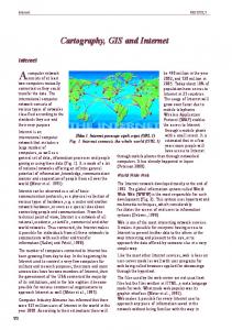
5.1 Principles of WebGIS A WebGIS is a common way of presenting dynamic maps online. It links the Internet with GIS technology. The GIS processing is performed online and maps are visualised in interactive web viewers. Although there are many ways in establishing a WebGIS, depending on the software components used, most applications are based on the same principles (Figure 9.8). The user works with a web client displayed in their Internet browser. The client contains the demanding GIS functions (e.g. zooming or panning), compiles the map requests and forwards them to the application server. The server passes the map requests to the mapserver, the central software performing the GIS processing. The mapserver, having access to the spatial data, executes the map requests and returns the maps as images to the web server, which finally sends them back to the user’s web mapping client. The application acts as a web-based information system. Another way is using a web service, for example a Web Map Service (WMS), a software function that is accessible by a desktop GIS programme providing direct access to the mapserver. WMS is a widely supported, standardised protocol for accessing maps online that contains the map request and parameters specifying GIS processing for the mapserver, for example choice of layers or spatial extent. The protocol standard is specified by the Open Geospatial Consortium (OGC), a non-profit international standards organisation with members from commercial, governmental and research organisations, including Google and Microsoft. It is leading the developments of standards to establish interoperability and ensures platform and software independent Server a) WebGIS

Forwarding

Map request

Browser (Web client)

Access Map server

Web server

Geodata

Map Map

b) Web service

Map request

Geodata

GIS (Local client)

Map

Data server (optional)

Figure 9.8 Simplified scheme of information and data transfer of a WebGIS and web service application.


287

Table 9.3 List of Several Open-Source (*) and Commercial Software Products Providing and Supporting the WMS Format WMS Servers Web Mapping Clients Desktop Clients

UMN Mapserver* GeoServer* Degree* ArcGIS Server ArcIMS GeoMedia Express Viewer ERDAS Apollo Server Demis Web Map Server

OpenLayers* Mapbender* ka-Map!* Mapbuilder* Chameleon* ArcGIS Explorer Autodesk MapGuide Oracle Map Viewer Worldkit ERDAS Titan

GRASS GIS* Quantum GIS* ArcGIS/ArcView ArcGlobe MapInfo Global Mapper Autodesk AutoCAD ERDAS Imagine uDig* OpenJUMP* Google Earth NASA World Wind Demis Mapper Gaja GDV Spatial Commander

usability of geospatial services and data sharing. WMS is one of the most frequently used protocols in web mapping, which is supported by many open-source and commercial software (Table 9.3). The introduction to all available software components for WebGIS applications would go beyond the scope of this chapter. One popular package available for Windows is Maptool’s ‘MapServer for Windows’ (www.maptools.org/ms4w/), which uses open-source components to provide a mapserver environment including libraries for data input and output. MapServer is GIS software running on a web server that enables interaction with GIS data over the Internet and generates cartographic output of geographic content. In addition, the Geospatial Data Abstraction Library (GDAL, www.gdal.org), a powerful tool for data translation and processing (which is used by several GIS programmes including GRASS, and ArcGIS) is included. An introduction to the most common WebGIS tools is given by Mitchell (2005). Figure 9.9 shows a WebGIS that visualises the results of a geomorphological field mapping campaign in the Turtmann valley (Switzerland), which is available online at www.geomorphology.at. The application employs MapServer generating the maps as WMS, the spatial database management system PostgreSQL (www.postgresql.org) maintaining the geometries and the web mapping client Mapbender (www.mapbender.

288


Figure 9.9 The graphical user interface (GUI) of the geomorphological WebGIS application Turtmanntal (Universities of Salzburg and Bonn, available at www. geomorphology.at).

org). Aerial images and a shaded relief map are provided as base layers and several thematic layers present information on process domains, surface materials, landforms and single processes. Due to MapServer’s powerful cartographic engine, complex geomorphological symbols can be implemented and displayed. Symbols based on the legend for high mountain systems established by Kneisel et al. (1998) have been implemented. The WebGIS map thus uses the same symbology as the printed map of the same area (Otto and Dikau, 2004). The MapServer uses one symbol file that defines the composition of symbols for all types of vector geometries. Point information, such as individual landforms, is displayed using a geomorphological font (Otto and Dikau, 2004) and the spatial orientation of each character is achieved by providing the rotation angle as attribute data. Line features, for example crests and ridges, are constructed using multi-level symbols and advanced polygon symbology is supported by hatching or image fills. The Turtmanntal WebGIS offers simple functionality of a desktop GIS such as spatial navigation, coordinate queries, length and area calculations as well as selection of single layers of information. The composed image of the map frame can be exported in highresolution PDF (300 dpi) in A4 and A3 landscape or portrait orientation. For educational purposes, a glossary delivers definitions of geomorphological terms.


289

The WMS online resources are accessible through an export tool and the maps can be embedded in other web or desktop GIS applications, thus the Turtmanntal WebGIS provides geospatial services as well. Figure 9.10 shows different applications of the same WMS services viewed in the original WebGIS application (a), as an overlay on Google Maps data in a web mapping application hosted on another server (b) and finally in two desktop GIS programmes, ESRI’s ArcMap (c) and Quantum GIS (d), both supporting the WMS format as a data source. The WMS protocol enables the easy implementation and integration of distributed WMSs from different servers and so the collection of huge “own data” pools becomes unnecessary. For simple visualisation of geomorphological data, a public WMS serving aerial photographs could be used as a base layer that is overlain with the WMS delivering the mapping results to produce the online geomorphological map (Figure 9.11).

(a)

(b)

(c)

(d)

Figure 9.10 An OGC-compliant WMS service in different web and desktop applications. (a) The original WebGIS application Turtmanntal (available at www.geomorphology.at), (b) as a WMS overlay on Google Maps data using the javascript library OpenLayers as web mapping client, (c) the WMS as data source in ArcGIS and (d) Quantum GIS.

290

(a)


(b)

(c)

Figure 9.11 A map based on distributed WMSs from different servers (a) Orthophoto WMS of the Bavarian Survey Administration showing the Reintal basin, Bavaria, Germany (WMS available at http://www.geodaten.bayern.de/ogc/getogc.cgi?), (b) WMS displaying the spatial distribution of sediment storages in the Reintal basin (available at www.reintal-webgis.de) and (c) the final map.

We believe that the value of geomorphological data increases the more it is linked to other available information. Geomorphologists should consider the opportunity to present and share their data in a way users can easily tie to other data sources.

5.2 Maps in Google Earth Google Earth is a free and convenient desktop application available for Windows and Mac OSX offering high performance access to global geographic data. The software provides an easy-to-use interface to a variety of data. Base data in Google Earth is the same as in the browser-based Google Maps application. A major difference lies in the way maps can be viewed and manipulated. Google Earth enables Earth image browsing in a three-dimensional view on a virtual globe (Brown, 2006). Butler (2006) noted Google Earth’s popularity to a growing number of scientists is due to its excellent background imagery and the ability to place spatial data on top of them. However, Google Earth has only limited analytic functions and it is not designed to replace professional GIS software. A tool like Google Earth increases researchers’ awareness to explore more powerful GIS techniques due to its easy visualisation (Butler, 2006). Google Earth uses the keyhole markup language (KML) to manage three-dimensional spatial data and also supports WMS as image overlays turning the application into a WMS client. KML, also an OGC standard, enables the organisation and exchange of vector geometries. Numerous tools, such as GDAL, are available for data translation into KML. KML handles each type of vector geometry differently; however, advanced visualisation by complex symbology is


291

limited. Point symbols are displayed as images, which enables a more complex symbology although data specific rotation is not possible. Line features are simply displayed with additional specifications of line width and colour, but multi-level symbols are not supported. Polygon features only support simple colour fills, with no hatching or patterned fills, and the style for polygon perimeters is the same as for line symbols (Figure 9.12). This restricts the use of KML for complex geomorphic feature visualisation and limits its suitability for the dissemination of geomorphological maps. As a rule of thumb, one should keep the symbology for a KML file as simple as possible (see Chapter 8 for further discussion on spatial data formats). One possible method to distribute geomorphological maps for Google Earth is to display the map as an image overlay. The image is exactly positioned on Google’s virtual globe by a bounding box. A single image will only be displayed at the scale the image was created and zooming will deliver blurred data. The best performance is achieved if the image is served as a network link through a WMS. The image is refreshed after each navigation task and delivers high resolution at different scales. The WMS map request can be embedded in a KML file and stored on a local hard drive. In addition, the use of Google Earth as a WMS client allows the display of additional information from any publicly available WMS. (a)

(b)

Figure 9.12 WMS overlays and the corresponding KML files in Google Earth. (a) Geomorphic features as WMS overlays in Google Earth. This lesser known feature allows the display of any publicly available WMS. The WMS appears as an image overlay that is refreshed after each navigation task. (b) The same data as a KML layer, the KML file was generated using the GDAL/OGR tool (GDAL, www.gdal.org). Compared to the WMS overlays, more sophisticated symbology like hatching, multilevel symbols or symbol rotation is not supported within the style reference of KML.

292


6. CONCLUSIONS The perception and mapping of landscapes is a subjective process. The usability and quality of geomorphological maps is therefore not only dependent upon the choice and familiarity of the legend system and symbols but also to a greater extent upon good map design. Cartography provides valuable principles and techniques to focus the reader’s attention to the main content of a map. To apply these principles, geomorphologists should be aware of the different cartographic elements that compose geomorphological maps and their usage when creating a map. Legibility is probably the greatest challenge to geomorphological maps. A clear hierarchical organisation, the thoughtful application of colour, contrast and symbol density and a well-balanced arrangement of map items are good preconditions for well-designed maps that deliver the intended message. This chapter has introduced many different legend and mapping systems. The choice often depends on the author’s scientific context or the purpose of the map. A legend system should be adjusted to the specific conditions of the study area and the message of the map, sometimes requiring the creation of new symbols. Due to recent advances in graphic and map design functionality, GIS software provides increasing possibilities for map creation and creative map design. However, graphics software still enables more flexible symbol generation and map creation. To make full use of GIS functionality, database structure, layer composition and data formats need to be considered prior to map creation. This enables not only the storage and distribution of data but also helps to create a clear hierarchical organisation of the map contents. The Internet is a valuable platform for storage, exchange and dissemination of geomorphological information. Web mapping is a central part of the Internet that can be used for geomorphological maps as well. Either by static or dynamic techniques, geomorphological maps are easily published online using free software and data. Interoperability and exchange of geomorphological maps and data are provided by data and protocol standards for web mapping (e.g. WMS). Publication of geomorphological data through the Internet will contribute to the distribution and application of geomorphological maps in other scientific and non-scientific fields. In order to assure that geomorphological maps deliver the information aimed for, whether through online or printed maps, a clear and understandable design and composition of the geomorphological map is required.


293

REFERENCES Barsch, D., Liedtke, H., 1980a. Methoden und Anwendbarkeit Geomorphologischer Detailkarten Beitra¨ge zum GMK-Schwerpunktprogramm II, Berliner Geographische Abhandlungen. Barsch, D., Liedtke, H., 1980b. Principles, scientific value and practical applicability of the geomorphological map of the Federal Republic of Germany at the scale of 1:25,000 (GMK 25) and 1:100,000 (GMK 100). Z. Geomorphol. Suppl. 36, 296 313. Barsch, D., Fra¨nzle, O., Leser, H., Liedtke, H., Sta¨blein, G., 1985. Geomorphological mapping in the Federal Republic of Germany. First International Conference on Geomorphology, Manchester. Barsch, D., Fischer, K., Sta¨blein, G., 1987. Geomorphological mapping of high mountain relief, Federal Republic of Germany (with geomorphological map Ko¨nigssee, scale 1:25.000). Mt. Res. Dev. 7, 361 374. Bertin, J., 1982. Semiology of Graphics. University of Wisconsin Press, Madison, WI. Brewer, C.A., 2009. Colorbrewer. ,http://www.ColorBrewer.org. (accessed September 2009). Brown, M.C., 2006. Hacking Google Maps and Google Earth. Wiley, Chichester. Butler, D., 2006. The web-wide world. Nature 439, 776 778. Cooke, R.U., Doornkamp, J.C., 1990. Geomorphology in Environmental Management. A New Introduction. Clarendon Press, Oxford. De Graaff, L.W.S., De Jong, M.G.G., Rupke, J., Verhofstad, J., 1987. A geomorphological mapping system at scale 1:10,000 for mountainous areas (Austria). Z. Geomorphol. 31, 229 242. Demek, J., Embleton, C., 1978. Guide to Medium-Scale Geomorphological Mapping. E. Schweizerbart’sche Verlagsbuchhandlung, Stuttgart. Demek, J., Embleton, C., Gellert, J.F., Verstappen, H.T., 1972. Manual of Detailed Geomorphological Mapping. International Geographical Union Commission on Geomorphological Survey and Mapping. Academia, Prague. Dykes, A., 2008. Geomorphological maps of Irish peat landslides created using hand-held GPS. J. Maps v2008, 258 276. Evans, I.S., 1990. Cartographic techniques in geomorphology. In: Goudie, A. (Ed.), Geomorphological Techniques. Unwin Hyman, London. Geilhausen, M., Otto, J.-C., Dikau, R., 2007. GMK.digital Geomorphologische Karten im Netz. ,http://gidimap.giub.uni-bonn.de/gmk.digital/home.htm. (accessed September 2009). Gilewska, S.K.M., 1968. Project of the Unified key to the geomorphological map of the World. Folia Geographica, Ser. Geographica-Physica, II. Polska Akademia Nauk, Krako´w. GITTA, 2006. Layout design settings/graphical semiology. Geographic Information Technology Training Alliance. ,http://www.gitta.info/LayoutDesign/en/html/ DefOrgMapEle_learningObject1.html. (accessed January 2010). Gustavsson, M., Kolstrup, E., 2009. New geomorphological mapping system used at different scales in a Swedish glaciated area. Geomorphology 110, 37 44. Gustavsson, M., Kolstrup, E., Seijmonsbergen, A.C., 2006. A new symbol-and-GIS based detailed geomorphological mapping system: renewal of a scientific discipline for understanding landscape development. Geomorphology 77, 90 111. Gustavsson, M., Seijmonsbergen, A.C., Kolstrup, E., 2008. Structure and contents of a new geomorphological GIS database linked to a geomorphological map with an example from Liden, central Sweden. Geomorphology 95, 335 349. Hake, G., Gru¨nreich, D., Meng, L., 2001. Kartographie. Visualisierung raum-zeitlicher Informationen. de Gruyter, Berlin.

294


Haq, B.U., Eysinga, F.W.B., 1987. Geological Time Table. Elsevier, Amsterdam. IGUL, 2010. La le´gende geómorphologique de l’IGUL. ,http://www.unil.ch/igul/ page40935.html. (accessed January 2010). Kienholz, H., 1976. Kombinierte geomorphologische Gefahrenkarte 1:10000 von Grindelwald. Catena 3, 265 294. Kienholz, H., 1978. Maps of geomorphology and natural hazards of Grindelwald, Switzerland: scale 1:10000. Arct. Antarct. Alp. Res. 10, 169 184. Kienholz, H., Krummenacher, B., 1995. Symbolbaukasten zur Kartierung der Pha¨nomene. Mitteilungen des Bundesamtes fu¨r Wasser und Geologie Nr. 6. Bern, Bundesamt fu¨r Umwelt, Wald und Landschaft (BUWAL). Klimaszewski, M., 1982. Detailed geomorphological maps. ITC J., 3, 265 271. Klimaszewski, M., 1990. Thirty years of geomorphological mapping. Geogr. Pol. 58, 11 18. Kneisel, C., Tressel, E., 2000. Zur Anwendung der neuen GMK Hochgebirge mit einer Beispielkartierung aus den Ostschweizer Alpen. Trierer Geographische Studien 23, 113 132. Kneisel, C., Lehmkuhl, F., Winkler, S., 1998. Legende fu¨r geomorphologische Kartierungen in Hochgebirgen (GMK Hochgebirge). Trierer Geographische Studien 18: 24S. Kraak, M.-J., Ormeling, F., 2002. Cartography: Visualization of Geospatial Data. Prentice Hall, Upper Saddle River, NJ. Krygier, J., Wood, D., 2005. Making Maps: A Visual Guide to Map Design for GIS. The Guilford Press, New York. Kugler, H., 1964. Großmaßsta¨bige Geomorphologische Kartierung und Geomorphologische Reliefanalyse. Universita¨t Leipzig, Leipzig, Dissertation. Kuhle, M., 1990. Quantificational reductionism as a risk in geography instanced by the 1:25000 Geomorphological map of the Federal Republic of Germany. Geogr. Pol. 58, 41 54. Lee, E.M., 2001. Geomorphological mapping. In: Griffiths, J.S. (Ed.), Land Surface Evaluation for Engineering Practice. The Geological Society, London, Special Publication No. 18. Longley, P.A., Goodchild, M.F., Maguire, D.J., Rhind, D.W., 2005. Geographic Information Systems and Science. Wiley, Chichester. Maarleveld, G.C., ten Cate, J.A.M., de Lange, G.W., 1977. Geomorfologische kaart van Nederland schaal 1:50 000. Legenda, 20pp 1 Toelichting op de legenda, 91 pp. Stichting voor Bodemkartering, Wageningen/Rijks Geologische Dienst, Haarlem. Mitchell, T., 2005. Web Mapping Illustrated. O’Reilly, Sebastopol, CA. Otto, J.-C., 2008. Symbols for geomorphologic mapping in high mountains for ArcGIS. ,http://www.geomorphology.at/index.php?option=com_content&task=view&id=133 &Itemid=176. (accessed September 2009). Otto, J.-C., Dikau, R., 2004. Geomorphic system analysis of a high mountain valley in the Swiss Alps. Z. Geomorphol. N.F. 48, 323 341. Passarge, S., 1912. Physiologische morphologie. Mitt. Geogr. Ges. Hamburg 26, 135 337. Robinson, A.H., Morrison, J.L., Muehrcke, P.C., Kimerling, A.J., Guptill, S.C., 1995. Elements of Cartography. Wiley, Chichester. Rouleau, B., 1993. Theory of cartographic expression and design. In: Anson, R.W., Ormeling, F.J. (Eds.), Basic Cartography, vol. 1: Manual Series Basic Cartography for Students and Technicians. Butterworth-Heinemann, Oxford, pp. 65 91. Salome´, A.I., Dorsser, H.J., Rieff, P.L., 1982. A comparison of geomorphological mapping systems. ITC J., 3.


295

Schoeneich, P., 1993. Comparison des syste´mes de le´gendes francais, allemand et suisse principes de la le´gende IGUL. In: Reynard, E., Schoeneich, P. (Eds.), Cartographie Geómorphologique, Cartographie des Risques, Travaux et Recherches, 9, pp. 15 24. Schoeneich, P., Reynard, E., Pierrehumbert, G., 1998. Geomorphological mapping in the Swiss Alps and Prealps. In: Kriz, K. (Ed.), Hochgebirgskartographie Silvretta ’98. Wiener Schriften zur Geographie und Kartographie, 11, pp. 145 153. Slocum, T.A., Mcmaster, R.B., Kessler, F.C., Howard, H.H., 2005. Thematic Cartography and Geographics Visualization. Prentice Hall, Upper Saddle River, NJ. Speight, J.G., 1974. A parametric approach to landform regions. Progress in Geomorphology, Special Publication. Institute of British Geographers, Oxford, pp. 213 229. St-Onge, D.A., 1981. Theories, paradigms, mapping, and geomorphology. Can. Geogr. 25, 307 315. Sta¨blein, G., 1980. Die Konzeption der Geomorphologischen Karten GMK25 und GMK100 im DFG-Schwerpunktprogramm. Berl. Geogr. Abhandlungen 31, 13 30. Theler, D., Reynard, E., 2008. Geomorphological maps of a high mountain watershed: sedimentary dynamics of the Bruchi torrent, Swiss Alp. J. Maps v2008, 289. Tricart, J., 1965. Principes et Methodes de la Geomorphologie. Masson, Paris, 465 pp. Verstappen, H.T., 1970. Introduction to the ITC System of Geomorphological survey. K. N.A.G. Geographisch Tijdschrift IV, 87 91. Verstappen, H.T., Zuidam, R.A., 1968. ITC Textbook of Photo-Interpretation, VII: 2-ITC System of Geomorphological Survey.