Author manuscript, published in "Journal of Applied Remote Sensing 2, 1 (2008) 023526" DOI : 10.1117/1.2957968
Change detection in synthetic aperture radar images with a sliding hidden Markov chain model Zied Bouyahiaa , Lamia Benyoussefb , and St´ephane Derrodeb a Ecole ´ Nationale des Sciences de l’Informatique,
hal-00325110, version 1 - 26 Sep 2008
Campus Universitaire de la Manouba, 2010 Manouba, Tunisia.
[email protected] b Institut Fresnel (CNRS UMR 6133), ´ UPCAM & Ecole Centrale Marseille, Technopˆole de Chˆateau-Gombert, 38, rue Fr´ed´eric Joliot Curie, 13451 Marseille Cedex 20, France.
[email protected] [email protected] Abstract. This work deals with unsupervised change detection in bi-date Synthetic Aperture Radar (SAR) images. Whatever the indicator of change used to compute the criterion image, e.g. log-ratio or Kullback-Leibler divergence between images, we have observed poor quality change maps for some events when using the Hidden Markov Chain (HMC) model we focus on in this work. The main reason comes from the stationary assumption involved in this model –and in most Markovian models such as Hidden Markov Random Fields–, which can not be justified in most observed scenes: changed areas are not necessarily stationary in the image. Besides the non-stationary Markov models proposed in the literature, the aim of this paper is to describe a pragmatic solution to tackle change detection stationarity by evaluating and comparing a 1D and a 2D window approaches. By moving the window through the criterion image, the process is able to produce a change map which can better exhibit non-stationary changes than the classical HMC applied directly on the whole criterion image. Special care is devoted to the estimation of the number of classes in each window, which can vary from one (no change) to three (positive change, negative change and no change) by using the corrected Akaike Information Criterion suited to small samples. The quality assessment of the proposed approaches is achieved with a pair of RADARSAT images bracketing the Mount Nyiragongo volcano eruption event in January 2002. The available ground truth confirms the effectiveness of the proposed approach compared to a classical HMC-based strategy. Keywords: Change Detection in SAR images, Hidden Markov chain, Unsupervised classification, EM estimation, MPM classification, Akaike Information Criterion.
1 INTRODUCTION Bi-date change detection in SAR images is known to be a challenging task, mostly from the speckle inherent to this modality, and many algorithms have been proposed the last years. Among the post-classification comparison and the joint classification methods, the main approach used to detect changes between two date SAR images consists in segmenting a criterion image that exhibits change. Examples of such indicator of change are image difference, image ratio/log-ratio, Kullback-Leibler divergence or sub-space projection [1–4] for examples. For segmentation, among the numerous available supervised or automatic classification methods (SVM, genetic algorithms...), methods based on Markovian assumptions (Markov random
hal-00325110, version 1 - 26 Sep 2008
fields [1, 5, 6], Markov chains [7, 8]) give encouraging results, for the same reasons that explain their nice SAR image segmentation performances [9]: the regularization effect of Markov models reduces the false detection rates consequently. However, for some observed scenes, Markovian models do not appear as efficient as expected to detect changes. The main reason comes from the stationary assumption involved in these models, which can not be justified in most observed scenes: changed areas are not necessarily stationary in the image. Besides the non-stationary Markov models proposed in the literature [10–13], the aim of this paper is to propose a pragmatic solution to improve the quality of change detection maps by relaxing the stationary assumption of Hidden Markov Chain (HMC), using a sliding window. By non-stationary, we mean to produce a class image in which the visual aspect of the spatial organization of the different classes varies with pixels. Originally [14, 15], the HMC model is applied on the image after its conversion to a 1D signal using the Hilbert-Peano scan [16] (see Fig. 1). Estimation and classification are performed on the signal, and the segmented image is reconstructed by using an inverse Peano scan. In this work, two strategies have been experimented, i.e. a block-window one and a sub-chain one. The block-window strategy consists in sliding a small square-shaped window (typically 16 × 16 pixels) over the entire image, and in applying the classical HMC model (after Hilbert-Peano scanning). In the sub-chain strategy, the criterion image is scanned pixel by pixel according to the Hilbert-Peano scan. For each pixel, we only consider a neighborhood of limited extend around it, e.g. 40 pixels before and 40 pixels after the pixel of interest. In both strategies, classical HMC parameter estimation is performed for each window Wn built these ways (i.e. whatever it is 1D or 2D) using an Estimation-Maximization (EM) procedure. Then, for the pixel n only, a Bayesian decision using the Marginal Posterior Mode (MPM) criterion is taken. By scanning entirely the criterion image (and using quick parameter update procedures to reduce computing time), the so-obtained change detection maps are able to exhibit non-stationary changes in the scene. These “windowed strategies” were motivated by a previous study [17] that shown the exponential decreasing influence of far-away pixels on so-called “forward” and “backward” probabilities used to estimate hidden parameters and to take MPM decision [18–20]. Special care is devoted to the estimation of the number of classes in each window, which can vary from one (no change) to three (positive change, negative change and no change) by using the corrected Akaike Information Criterion (AICc). Indeed, it is known to be more robust than AIC and BIC (Bayesian Information Criterion) in case of small samples [21, 22]. Data-driven densities, which model the noise of classes are supposed to be Gaussian in this work. Other kinds of distributions remain possible [15, 23] but the Gaussian choice was primarily motivated by the small size of windows involved int he local approaches and so the few number of samples available for parameters estimation. The remaining of the paper is organized as follows: Section 2 recalls basic facts about HMC-based unsupervised image segmentation using EM for parameters estimation and MPM for Bayesian classification. Section 3 explains how the modified HMC models, which exploit a local window strategy, can be used to reduce the impact of stationarity assumption for change detection. Section 4 presents change maps obtained on a couple of Radarsat images bracketing the Mount Nyiragongo eruption event in January 2002, using log-ratio and Kullback-Leibler divergence criteria as indicators of change. An available ground-truth enables to measure the benefit and compare the two methods, with respect to the original HMC model, in term of classification error rates.
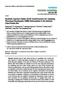
2 UNSUPERVISED SEGMENTATION USING HMC This section is intended to give some recalls about the HMC model [20] and its use for unsupervised image segmentation [14, 15]. The HMC model can be adapted to a 2D analysis through a Hilbert-Peano scan of the image, see Fig. 1. Hence all estimation and segmentation processings
1 2 3 4 5 6 7 8 1 2 3 4 5 6 7 8 y y1
yn−1 yn yn+1
yN
hal-00325110, version 1 - 26 Sep 2008
Fig. 1: Hilbert-Peano scan construction for an 8 × 8 image. This scan is used to transform a 2D image into a 1D signal (y), and conversely.
are applied on the 1D sequence, and the segmented 2D image is reconstructed by using a reverse Hilbert-Peano scan from the 1D classified sequence. 1- Model: An image y = {y1 , . . . , yN }, N being the total number of pixels, is considered as a realization of the 1D observed process Y = {Y1 , . . . , YN }, each Yn is a real-valued random variable. The segmented image x = {x1 , . . . , xN } is considered as a realization of a hidden process X = {X1 , . . . , XN }, each Xn ∈ Ω = {1, . . . , K} is a discrete random variable. In classical HMC modeling, X is assumed to be a Markov chain, i.e. p (xn+1 | xn , . . . , x1 ) = p (xn+1 | xn ) . The distribution of X is consequently determined by the distribution of X1 , denoted by πk = p (X1 = k), and the set of transition matrices (An )1≤n≤N whose entries are anij = p (Xn+1 = j | Xn = i). We further assume that X is a stationary Markov chain, i.e. entry anij = aij does not depend on n. With the QNfollowing additional properties: (i) Yn are independent conditionally to X, i.e. p (y | x) = n=1 p (yn | x), and (ii) p (yn | x) = p (yn | xn ), the distribution of the pairwise process (X, Y) can be written as p (x, y) = πx1 fx1 (y1 )
N Y
axn−1 ,xn fxn (yn ),
n=2
with fxn (yn ) = p (yn | xn ) the data-driven densities, which are assumed to be Gaussian in this work (see Giordana et al [15] for generalized mixtures). 2- Classification: The estimation of X from Y can be done by applying the MPM Bayesian criterion: ∀n ∈ [1, . . . , N ], x bnMPM (y) = arg max ξn (k), (1) k∈Ω
with ξn (k) = p (Xn = k | y) the marginal a posteriori probabilities. The HMC model allows explicit computation of the MPM solution using the well-known Baum’s “forward” αn (k) and “backward” βn (k) probabilities [18], modified by Devijver [19] for computational reasons: αn (k) = βn (k) =
p (Xn = k|y1 , . . . , yn ) , p (yn+1 , . . . , yN |Xn = k) . p (yn+1 , . . . , yN | y1 , . . . , yn )
Such probabilities can be computed recursively: Forward probabilities • Initialization: for n = 1, ∀k ∈ Ω,
πk fk (y1 ) . α1 (k) = X πl fl (y1 )
(2)
l∈Ω
• Induction: for 2 ≤ n ≤ N , fk (yn ) ∀k ∈ Ω,
αn (k) = X
X
αn−1 (l) alk
l∈Ω
X
fi (yn )
i∈Ω
.
αn−1 (l) ali
(3)
l∈Ω
Backward probabilities • Initialization: for n = N , ∀k ∈ Ω,
hal-00325110, version 1 - 26 Sep 2008
• Induction: for 1 ≤ n ≤ N − 1,
∀k ∈ Ω,
βn (k) = X
1 . K
akl fl (yn+1 ) βn+1 (l)
l∈Ω
βn (k) = X
fi (yn+1 )
i∈Ω
X
αn (l) ali
.
l∈Ω
It can be shown that marginal a posteriori probabilities involved in MPM classification can be written ξn (k) = αn (k) βn (k), (4) and joint a posteriori probabilities ψn (k, l) = p (Xn = k, Xn+1 = l | y) as: αn (k) βn+1 (l) akl fl (yn+1 ) . ψn (k, l) = X X αn (i) βn+1 (j) aij fj (yn+1 )
(5)
i∈Ω j∈Ω
3- Estimation: Before classification, all parameters involved in the CMC model θ = {πk , akl , fk }k,l∈Ω ,
(6)
have to be estimated. One well-known solution is to use the EM iterative procedure [24] aiming at optimizing the log-likelihood of data, according to the steps described in Algorithm 1, with following update equations N −1 X
∀k ∈ Ω,
π ck
[q]
N X
∀k ∈ Ω,
µ ck
[q]
=
N 1 X [q] = ξ (k); N n=1 n
∀k, l ∈ Ω,
[q]
[q]
N X
ξn[q] (k) yn
n=1
ac kl
;
∀k ∈ Ω,
c2 σ k
[q]
=
=
Ψn[q] (k, l)
n=1
ξn[q] (k)
Nπ ck
[q]
³ yn − µ ck
.
[q]
n=1 [q]
Nπ ck Nπ ck Iterative estimation of parameters is stopped when parameters do not vary much.
(7) ´2 .
(8)
Algorithm 1 HMC parameters estimation using EM. q ← 0: Initialize parameters θ[0] repeat -q ←q+1 [q] [q] - Compute “Forward” αn and “Backward” βn probabilities using equations (2) to (2). [q] [q] - Compute a posteriori probabilities ξn (k) using eq. (4) and ψn (k, l) using eq. (5). - Estimate CMC parameters θ[q] using eq. (7) for Markov parameters and eq. (8) for Gaussian data-driven parameters. until kθ[q] − θ[q−1] k < Threshold.
hal-00325110, version 1 - 26 Sep 2008
3 HMC ON A SLIDING WINDOW As mentioned above, unsupervised image segmentation using HMC is performed with the assumption that the Markov chain is stationary, which means that only one set of parameters θ, cf. Eq. (6), governed the whole segmented image. When the hidden chain is non-stationary, the unsupervised restoration results using the HMC model can be poor, due to a bad match between the real and estimated models. Several methods have been proposed to avoid this weakness. The initial work by Ferguson, called “variable duration Hidden Markov Model (HMM)”, models the class durations by various types of probability distributions [25]. Latter, the state transition probabilities are explicitly modeled as functions of time [10] and, therefore, are referred to as non-stationary HMM. The difficult problem of parameters estimation can be solved using a Markov Chain Monte Carlo (MCMC) sampling scheme as proposed by Djuric et al [11]. Then, further generalizations to hidden semi-Markov chains have been proposed [12], and the use of the theory of evidence and Dempster-Shafer fusion in the so-called “Triplet Markov Chain” (TMC) framework [13]. We propose here two simple and pragmatic algorithms to tackle the stationarity assumption, while preserving the Markov regularization effect. In a first approach, called sub-chain, the entire criterion image is scanned pixel by pixel according to the Hilbert-Peano scan [16]. For each pixel n of the image, 1 ≤ n ≤ N , we only consider a neighborhood of limited extend around it, e.g. 40 pixels before and 40 pixels after the pixel of interest (λ = 125, and Nw = 2λ + 1 = 251), see Fig. 2. The second strategy, called block-window, consists in sliding a small square-shaped window Wn (typically 16×16 pixels, Nw = 256) centered on each pixel n of the criterion image. The windows is then transformed according to the Hilbert-Peano scan in order to be processed by the HMC model. HMC parameter estimation is then performed for each window Wn built these ways using the EM procedure described in Algorithm 1 of Section 2. Then, for the pixel n only, a Bayesian decision using the MPM criterion in Eq. (1) is taken. By scanning entirely the criterion image, we estimate as many sets of parameters θ as the number of windows (which is equal to N ): n o [n] [n] [n] θ[n] = πk , akl , fk , n ∈ [1, . . . , N ]. k,l∈Ω
Hence, while we consider a CMC of limited extent centered on each pixel, we produce a segmented image which exhibits non-stationary classes in the scene, i.e. in which the visual aspect of the spatial organization of the different classes varies with pixels. From a computing resources point-of-view, the memory required for the local HMC models is limited to the memory necessary for an HMC with Nw ¿ N pixels. On the other hand, much more parameters have to be estimated, but with however small sample size (Nw ). Hence the two sliding window models will be able to deal with the very big images (more than 10000 × 10000 pixels) awaited for the next generation of sensors, which is not the case of the classical HMC modeling. To reduce computing time, we have implemented a quick parameters update
hal-00325110, version 1 - 26 Sep 2008
Fig. 2: Principle of the sub-chain HMC model.
procedure that initializes HMC parameters of widows Wn from HMC parameters obtained at convergence from the window Wn−1 . Hence, only very few iterations are required for the EM to converge. Using these windowed approaches, one difficulty arises for the estimation of the number of classes Kn in each Wn . Indeed, if the number of classes in the whole criterion image is known to be K = 3, corresponding to negative change, no change and positive change, Kn may vary between 1 and 3 from one window to the other and should be estimated in each window. This problem is known as “model or order selection” in the literature. Among information criteria available, we find BIC (Bayesian Information Criterion) and AIC (Akaike Information Criterion) which can be written in the windowed context considered here as ³ ´ BICKn = −2 ln L y; θˆKn + dKn ln (Nw ) , ³ ´ AICKn = −2 ln L y; θˆKn + 2 dKn , where • dKn denotes the number of free parameters of the model with order Kn (dKn = 3Kn − 1 under Gaussian assumption), • θˆKn the estimated parameters for the model of order Kn , • L(.) the likelihood function for the estimated model with parameter θKn . Instead of these criteria, we used the corrected AIC criterion defined by ³ ´ AICcKn = −2 ln L y; θˆKn + 2
Nw dKn , Nw − dKn − 1
(9)
which is known to be more robust than AIC and BIC in case of small samples [21, 22].
4 CHANGE DETECTION IN A (F5,F2) COUPLE OF RADARSAT IMAGES This section is intended to evaluate the two local segmentation approaches, and the benefit of relaxing the stationarity assumption of the HMC model. The application consists in detecting lava pathes after the Mount Nyiragongo eruption event in January 2002, which has destroyed a
hal-00325110, version 1 - 26 Sep 2008
(a) Before, Mar. 22 2001, Ib
(b) After, Jan. 21 2002, Ia
(c) Ground-truth
Fig. 3: Excerpts of two RadarSat images of Mount Nyiragongo volcano before and after the January 2002 eruption.
part of Goma city, including the airport (Democratic Republic of Congo). A partial analysis of the sub-chain algorithm on simulated SAR images is reported in [26]. Figure 3 shows the two Fine-Beam RadarSat images used to assess changes, together with the available ground-truth. Image “before” and “after” are respectively F5 and F2 images, with incidence angles of 49 and 35 degrees. Since the angles of incidence are not the same, interferometric conditions are not respected and coherence between the two is not exploitable. The ground-truth was obtained from an accurate study conducted by French National Spatial Center (CNES) from a request by the Belgian Civil Protection, inside the “International Charter for Space and Major Disasters” framework. (The site http://www.disasterscharter. org/disasters/congo_e.html shows images and/or image products delivered under the Charter.) It is based on many different modalities, e.g. Aster, Landsat, Spot and RadarSat images, with data collected in situ [27]. Authors of this study pointed out several weaknesses on actual methods ; the windowed HMC models is a partial answer to the unsuitability of classical Markov models to deal with such operational data and framework (very large images and nonstationarity of changes). Both images have a ground resolution of 10m covering an area of 4Km in azimuth direction and 8Km in range direction. Images were orthorectified by IGN-F (French National Geographic Institute) to a UTM35S projection, as for the ground-truth map shown in Fig. 3(c). Neither filtering nor calibration was applied. We follow on this scene the evolution of lava flow which arises from the summit of the volcano on top of the image and flows straight down to cover a part of a landing strip and Goma City (including the airport), and ending in sea. Lava flows from this event are really difficult to detect with radar images since, in some cases, the lava surface was very rough, so it appears as a radiometry increase in the change detection. In some other cases its surface is rather smooth, producing a decrease or even no change of radiometry in the change detection. Experiments are conducted with the classical mean log-ratio detector (MLRD) and the Gaussian Kullback-Leibler distance (GKLD). These detectors are computed for each pixel (i, j) us-
hal-00325110, version 1 - 26 Sep 2008
(a) MLRD
(b) GKLD
Fig. 4: Criterion images obtained using the mean log-ratio detector and the Gaussian Kullback-Leibler distance.
ing a window w centered on it. If we denote by µb , µa , σb and σa the local mean values and local standard deviations of the Ib and Ia images computed on w, we get for the two criterions µ ¶ µb ILR (i, j) = log , (10) µa and IKL (i, j) =
σb4 + σa4 + (µb − µa )2 (σb2 + σa2 ) − 1. 2 σb2 σa2
(11)
The size of w should not be too small to guarantee enough samples, nor too big to avoid too much filtering. Fig. 4 presents the criterion images so obtained for w = 35 × 35, which appears as a good compromise. We performed the classification of the criterion images in Fig. 4 with the classical HMC model, the sub-chain approach and the block-window strategy. For all experiments, we considered K = 3 classes corresponding to NC, C+ and C-. For the local approaches, the number of classes, between 1 and 3, is estimated for each position of the window by using the AICc order selection criterion in eq. (9). Classes C+ and C- were then fused to obtain a binary change map comparable to the ground-truth. Fig. 5 presents the Receiver Operating Characteristics (ROC) curves, i.e the False Alarm Rate (FAR) versus the False Rejection Rate (FRR), for different sizes of W . These rates are computed by comparison of the segmented images with the ground-truth. As expected, the change detection accuracy evolves with W , in a way very similar for the two window approaches. For the GKLD criterion, the optimal values of Nw is about 251 (λ = 125) and 256 (16 × 16), because it gives the best compromise between FAR and FRR. Fig. 6 shows the binary maps obtained for the three models and the two criterions. For the MLRD criterion, the results are about the same, while more difficult to observe. It should be noted that the LMRD criterion gives a lower rejection rate than the GKLD one, but also a small higher acceptance rate. On the other hand, the classical HMC model gives, almost each time, the lowest FRR but also the highest FAR, producing a total error rate substantially
hal-00325110, version 1 - 26 Sep 2008
(a) Sub-Chain
(b) Block-Window
Fig. 5: ROC curves obtained with the two windowed HMC models under Gaussian distributions assumption, according to the window size Nw , and the two criterions (up: GKLD; down: MLRD). Table 1: Misclassification rates for two classic classification algorithms.
Algorithms K-means Bayesian decision
GKLD 39.2% 30.7%
MLRD 27.5% 25.7%
higher for the HMC model than for the two local strategies (see percentages of error reported in Fig. 6). So the choice of the criterion should be decided based on the level of confidence for the targeted application. The benefit of using the local approaches can be directly observed from the difference of error rates with the HMC model. Indeed, a decreasing of about 26% for the GKLD criterion and 33% for the MLRD criterion is observed for this scene. This can be directly attributed to the weakening of the stationarity assumption of the local approaches. However the change maps obtained do not allow to detect precisely all the lava pathes and improvements need to be further proposed. For comparison purposes, we tried two classical unsupervised classification algorithms: the K-means algorithm and the Bayesian decision using EM/Gaussian for parameters estimation. Results are reported in Table 1. Whatever the criterion used, the error rates are significantly higher for these two methods than for the local strategies and also for the classical HMC model. This can be explained by the fact that K-means and Bayesian decision are blind methods, i.e. they do not take into account the neighborhood for classification for better regularization.
hal-00325110, version 1 - 26 Sep 2008
GKLD
τ = 14.0%
τ = 13.8%
τ = 20.7%
τ = 16.5% (a) Sub-Chain
τ = 16.9% (b) Block-Window
τ = 22.5% (c) Classical
MLRD
Fig. 6: Binary change detection maps obtained with the two windowed HMC models (a and b), and the classical HMC model (c) for the two criterions. τ is the total error rates. The window size was set to the optimal value obtained from the ROC curves (251 and 256).
Finally, to get an idea on the models complexity, Table 2 reports the mean computation times for the two windowed models and the classical HMC one. The two local models perform significantly quicker than the classical one.
5 CONCLUSION The unsupervised detection of changes from SAR data taken at different angles of incidence is a very challenging task, for which classical algorithms fail. Markov models, such as hidden Markov random fields or hidden Markov chains, are known to be very efficient to tackle the speckle, but the stationarity assumption they rely on can not be justified in most observed scenes.
Table 2: Mean computation times to estimate parameters and segment a criterion image for the classical HMC model and for the two local HMC models (with a window size of about 250 pixels each). Experiments have been conducted on an Intel Pentium IV with 1.66GHz processor and 512Mo of RAM.
hal-00325110, version 1 - 26 Sep 2008
Model Time
Classical HMC 5 min. 11 sec.
Sub-chain window 3 min. 42 sec.
Block-window 4 min. 06 sec.
This is the case of the (F5,F2) couple of RadarSat images bracketing the Mount Nyiragongo eruption, which occurred in January 2002. To overcome the stationarity assumption, we proposed two local versions of the HMC model, based on 1D (sub-chain) or 2D (block-window) sliding windows. Corrected AIC criterion was used to estimate the number of classes (between 1 and 3) at each position of the window. These algorithms allow to take into account non-stationarities in images since model parameters are estimated locally, and not globally as for the original model. Furthermore, the windowed approaches hold two characteristics interesting for applications and operational context: (i) they allows to process very large images which is not the case of Markovian models, and (ii) they do not require to tune parameters. Indeed, the question of an optimal size for the sliding windows is an open issue and depends on the image content. However a size of about 250 pixels seems to be acceptable, whatever the window strategy. Experiments were conducted using two classical detectors, i.e. the mean log-ratio and the Kullback-Leibler distance. Each time the total error rates, computed from a ground-truth of the eruption scene, are substantially lower than for the classical HMC model (about 30%). This illustrates the benefit of weakening the stationarity assumption of the original HMC model for change detection. However, from a thematic point of view, the results are not enough satisfactory and reasons why need to be further investigated.
Acknowledgments The authors are grateful to the anonymous reviewers for their constructive suggestions.
References [1] L. Bruzzone and D. F. Prieto, “Automatic analysis of the difference image for unsupervised change detection,” IEEE Trans. Geosci. Rem. Sens. 38(3), 1171–1182 (2000). [doi:10.1117/12.154577]. [2] E. J. M. Rignot and J. J. V. Zyl, “Change detection techniques for ERS-1 SAR data,” IEEE Trans. Geosci. Rem. Sens. 31(4), 896–906 (1993). [doi:10.1109/36.239913]. [3] J. Inglada and G. Mercier, “A new statistical similarity measure for change detection in multitemporal SAR images and its extension to multiscale change analysis,” IEEE Trans. Geosci. Rem. Sens. 19(5), 465–475 (2007). [doi:10.1109/TGRS.2007.893568]. [4] N. Nasrabadi, M. Tates, and H. Kwon, “Change detection methods for identification of mines in synthetic aperture radar imagery,” J. Appl. Remote Sens. 1, 013525 (2007). [doi:10.1117/1.2776947]. [5] T. Kasetkasem and P. K. Varshney, “An image change detection algorithm based on Markov random field models,” IEEE Trans. Geosci. Rem. Sens. 40(8), 1815–1823 (2002). [doi:10.1109/TGRS.2002.802498]. [6] F. Melgani and Y. Bazi, “Robust unsupervised change detection with Markov random fields,” in IEEE Int. Geosci. and Rem. Sens. Symp., 208–215 (2006). [doi:10.1109/IGARSS.2006.58].
hal-00325110, version 1 - 26 Sep 2008
[7] S. Derrode, G. Mercier, and W. Pieczynski, “Unsupervised change detection in SAR images using a multicomponent HMC model,” in MultiTemp’03, (Ispra, Italy) (2003). [doi:10.1142/9789812702630 0021]. [8] C. Carincotte, S. Derrode, and S. Bourennane, “Unsupervised change detection on SAR images using fuzzy hidden Markov chains,” IEEE Trans. Geosci. Rem. Sens. 44(2), 432– 441 (2006). [doi:10.1109/TGRS.2005.861007]. [9] R. Fjørtoft, Y. Delignon, W. Pieczynski, M. Sigelle, and F. Tupin, “Unsupervised segmentation of radar images using hidden Markov chain and hidden Markov random fields,” IEEE Trans. Geosci. Rem. Sens. 41(3), 675–686 (2003). [doi:10.1109/TGRS.2003.809940]. [10] B. Sin and J. H. Kim, “Nonstationary hidden Markov model,” Signal Process. 46, 31–46 (1995). [doi:10.1016/0165-1684(95)00070-T]. [11] P. M. Djuric and J. H. Chun, “An MCMC sampling approach to estimation of nonstationary hidden Markov models,” IEEE Trans. Signal Process. 50(5), 1113–1123 (2002). [doi:10.1109/78.995067]. [12] S.-Z. You and H. Kobayashi, “A hidden semi-Markov model with missing data and multiple observation sequences for mobility tracking,” Signal Process. 83, 235–250 (2003). [doi:10.1016/S0165-1684(02)00378-X]. [13] P. Lanchantin and W. Pieczynski, “Unsupervised restoration of hidden non stationary Markov chain using evidential priors,” IEEE Trans. Signal Process. 53(8), 3091–3098 (2005). [doi:10.1109/TSP.2005.851131]. [14] B. Benmiloud and W. Pieczynski, “Estimation des param`etres dans les chaˆınes de Markov cach´ees et segmentation d’images,” Traitement du Signal 12(5), 433–454 (1995). [15] N. Giordana and W. Pieczynski, “Estimation of generalized multisensor hidden Markov chains and unsupervised image segmentation,” IEEE Trans. Pattern Anal. Mach. Intell. 19(5), 465–475 (1997). [doi:10.1109/34.589206]. [16] W. Skarbek, “Generalized Hilbert scan in image printing,” in Theoretical Foundations of Computer Vision, Akademik Verlag, Berlin (1992). [17] S. Derrode, L. Benyoussef, and W. Pieczynski, “Contextual estimation of hidden Markov chains with application to image segmentation,” in IEEE Int. Conf. on Acoustics, Speech, and Signal Processing, 2 (2006). [doi:10.1109/ICASSP.2006.1660436]. [18] L. Baum, T. Petrie, G. Soules, and N. Weiss, “A maximization technique occurring in the statistical analysis of probabilistic functions of Markov chains,” Ann. Math. Stat. 41(1), 164–171 (1970). [doi:10.1214/aoms/1177697196]. [19] P.-A. Devijver, “Baum’s Forward-Backward algorithm revisited,” Pattern Recogn. Lett. 3, 369–373 (1985). [doi:10.1016/0167-8655(85)90023-6]. [20] L. R. Rabiner, “A tutorial on HMMs and selected applications in speech recognition,” Proc. IEEE 77(2), 257–286 (1989). [doi:10.1109/5.18626]. [21] N. Sugiura, “Further analysis of the data by Akaike’s information criterion and the finite corrections,” Comm. Stat. Theor. Meth. 7(1), 13–26 (1978). [doi:10.1080/03610927808827599]. [22] C. M. Hurvich and C.-L. Tsai, “Regression and time series model selection in small samples,” Biometrika 76(2), 297–307 (1989). [doi:10.1093/biomet/76.2.297]. [23] S. Derrode, G. Mercier, J.-M. Le Caillec, and R. Garello, “Estimation of sea-ice SAR clutter statistics from Pearson’s system of distributions,” in IEEE Int. Geosci. and Rem. Sens. Symp., 190–192 (2001). [doi:10.1109/IGARSS.2001.976098]. [24] A. P. Dempster, N. M. Laird, and D. B. Rubin, “Maximum likelihood from incomplete data via the EM algorithm,” J. Roy. Stat. Soc. 39(1), 1–38 (1977).
[25] J. D. Ferguson, “Variable duration models for speech,” in Proc. Symp. Appl. Hidden Markov Models Text Speech, 143179 (1980). [26] Z. Bouyahia, L. Benyoussef, and S. Derrode, “Unsupervised SAR images change detection with hidden Markov chains on a sliding window,” in Proc. SPIE, 6748, 674816 (2007). [doi:10.1117/12.737313]. [27] J. Inglada, J.-C.Favard, H. Yesou, S. Clandillon, and C. Bestault, “Lava flow mapping during the Nyiragongo January, 2002 eruption over the city of Goma (D.R. Congo) in the frame of the international charter space and major disasters,” in IEEE Int. Geosci. and Rem. Sens. Symp., 1540–1542 (2003). Z. Bouyahia: biography not available. L. Benyoussef: biography not available.
hal-00325110, version 1 - 26 Sep 2008
S. Derrode: biography not available.