Aug 17, 2005 - The stratosphere starts just above the troposphere and extends to 50 kilometers (31 miles) high. Compared to the troposphere, this part of the.
MODIS products and its study for Atmospheric applications
A Pilot Project Report for the partial fulfillment of Post Graduate Degree in Physics
Submitted by: MR.SANDEEP M.Sc (Physics) IVth Semester Mizoram University
Supervised by : Dr.YOGESH KANT Scientist CSSTEAP IIRS
INDIAN INSTITUTE OF REMOTE SENSING (Dept. of Space, Govt. of India) 4, Kalidas Road , DEHRADUN
i
INDIAN INSTITUTE OF REMOTE SENSING (Dept. of Space, Govt. of India) 4, Kalidas Road , DEHRADUN
Certificate
This is to certify that Mr.Sandeep has carried out a Project Study entitled, “MODIS products and its study for Atmospheric applications”, towards the partial fulfillment of Post Graduate degree in Physics from Mizoram University. This work has been carried out at the Centre for Space Science Technology and Education in Asia and the Pacific, Indian Institute of Remote Sensing, Dehradun. During participation his conduct was good. I wish him a bright future.
Date : 17th August , 2005
Dr.Yogesh Kant Project supervisor Scientist IIRS
Place : Dehradun
iii
CONTENTS
CHAPTER
PAGE NO.
Acknowledgement……………………………………………………i Certificate……………………………………………………………iii
CHAPTER 1
Introduction
1
CHAPTER 2
Remote sensing of the Atmosphere
4
CHAPTER 3
Atmospheric Aerosols
15
CHAPTER 4
Terra & Aqua Space Platforms
22
CHAPTER 5
The MODIS Sensor
29
CHAPTER 6
MODIS Products
37
References………………………………………………………….45
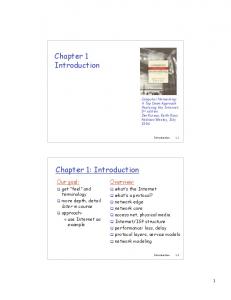
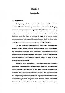
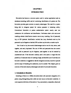
CHAPTER 1: INTRODUCTION Earth’s Atmosphere The Earth is surrounded by a blanket of air, which is called the Atmosphere. It reaches over 360 kilometers from the surface of the Earth, so one is only able to see what occurs fairly close to the ground. Early attempts at studying the nature of the atmosphere used clues from the weather, the beautiful multi-colored sunsets and sunrises, and the twinkling of stars. With the use of sensitive instruments from space, one is able to get a better view of the functioning of our atmosphere. Life on Earth is supported by the atmosphere, solar energy, and our planet's magnetic fields. The atmosphere absorbs the energy from the Sun, recycles water and other chemicals, and works with the electrical and magnetic forces to provide a moderate climate. The atmosphere also protects us from high-energy radiation and the frigid vacuum of space. The envelope of gas surrounding the Earth changes from the ground up. Four distinct layers have been identified using thermal characteristics (temperature changes), chemical composition, movement, and density.
Figure 1 : Layers of the Earth’s atmosphere
1
Troposphere The troposphere starts at the Earth's surface and extends 8 to 14 kilometers high (5 to 9 miles). This part of the atmosphere is the most dense. As one climbs higher in this layer, the temperature drops from about 17 to 52 degrees Celsius. Almost all weather is in this region. The tropopause separates the troposphere from the next layer. The tropopause and the troposphere are known as the lower atmosphere. Stratosphere The stratosphere starts just above the troposphere and extends to 50 kilometers (31 miles) high. Compared to the troposphere, this part of the atmosphere is dry and less dense. The temperature in this region increases gradually to -3 degrees Celsius, due to the absorbtion of ultraviolet radiation. The ozone layer, which absorbs and scatters the solar ultraviolet radiation, is in this layer. Ninety-nine percent of "air" is located in the troposphere and stratosphere. The stratopause separates the stratosphere from the next layer. Mesosphere The mesosphere starts just above the stratosphere and extends to 85 kilometers (53 miles) high. In this region, the temperatures again fall as low as -93 degrees Celsius as one increases in altitude. The chemicals are in an excited state, as they absorb energy from the Sun. The mesopause separates the mesophere from the thermosphere.The regions of the stratosphere and the mesosphere, along with the stratopause and mesopause, are called the middle atmosphere by scientists. This area has been closely studied on the ATLAS Spacelab mission series. Thermosphere The thermosphere starts just above the mesosphere and extends to 600 kilometers (372 miles) high. Temperatures in this region can go as high as 1,727 degrees Celsius. Chemical reactions occur much faster here than on the surface of the Earth. This layer is known as the upper atmosphere. The upper and lower layers of the thermosphere have been studied more closely during the Tethered Satellite Mission (TSS-1R).
2
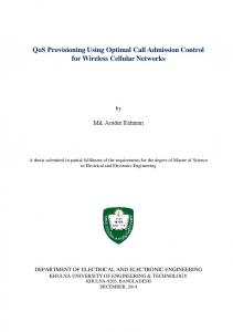
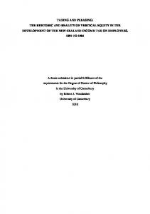
Composition of the Atmosphere The atmosphere is primarily composed of Nitrogen (N2, 78%), Oxygen (O2, 21%), and Argon (Ar, 1%). A myriad of other very influential components are also present which include the water (H2O, 0 - 7%), "greenhouse" gases or Ozone (O, 0 - 0.01%), Carbon Dioxide (CO2, 0.01-0.1%),as shown in Figure 2.
Figure 2
Beyond the Atmosphere The exosphere starts at the top to the thermosphere and continues until it merges with interplanetary gases, or space. In this region of the atmosphere, Hydrogen and Helium are the prime components and are only present at extremely low densities. Protection of the Atmosphere Numerous volatile halogen compounds are produced by man for industrial purposes. To some extent these substances end up in the atmosphere, and some of them persist for long periods, often centuries. Often, the effects of these substances on the atmosphere are non-negligible. For instance, these substances contribute to the depletion of the ozone layer or to increasing the greenhouse effect. Hence, the protection of the atmosphere consists in elaborating and implementing measures to reduce the impact of two groups of substances on the atmosphere: •
Substances that deplete the ozone layer: halons, CFCs, HCFCs, methyl bromide, carbon tetrachloride, trichloroethane, bromochloromethane • Synthetic greenhouse gases: HFCs, PFCs, SF6, also known as atmospherically persistent substances. 3
CHAPTER 2 : Remote Sensing of the Atmosphere This chapter deals with the ways of obtaining information about the atmosphere by Remote sensing. To do this, the wavelengths at which the atmosphere emits (and therefore also absorbs) are considered.
Composition Air is a mixture of gases. In the bulk of the atmosphere the air currents stir this mixture to a uniform composition much faster than diffusive separation under gravity can separate the constituents out. Some constituents have sources and sinks which produce noticeable changes. In particular the processes of evaporation and condensation of water vapour are quite rapid. It is convenient therefore to consider air as a mixture of dry air and water vapour. The composition of dry air is fairly constant and is as appears in the table.
*var indicates that the quantities of this constituentare variable Above about 80km oxygen begins to be dissociated by UV radiation from the sun. At still greater heights nitrogen also dissociates.
4
Mixing ratios The ratio of some importance is the mass of a constituent in an air sample to the total mass of the sample. This ratio is usually called the mass mixing ratio. There is an analogous quantity in terms of the number of molecules. As the volume of a gas at a standard pressure and temperature is proportional to the number of molecules (and independent of the substance) this ratio has come to be known as the volume mixing ratio. Thus the volume mixing ratio is defined as the number of molecules of a constituent in an air sample to the total number of dry air molecules in the sample. Note that the volume mixing ratio is also called the mole fraction, which is in many ways a better term, but “volume mixing ratio” is too firmly entrenched for it to be abandoned. Some variations on this terminology may be found. In particular, meteorologists use the term mixing ratio to mean the ratio of the mass of water vapour contained in an air sample to the mass of dry air with which it is mixed. Likewise some authors define mass mixing ratio of a pollutant as the ratio of the mass of pollutant to the total mass of air excluding the pollution. For pollutants which appear in only tiny quantities the difference between the two definitions will be negligible. (Mass mixing ratios of water vapour rarely exceed 40g/kg. So the difference between the two definitions of mass mixing ratio does not exceed 4%.) For minor constituents the mixing ratios will often be expressed in parts per million by volume (denoted as `ppmv') or analogously by mass. Thus the mixing ratio of hydrogen in dry air is 50 ppmv or 3.5 ppmm. The principal variable constituent of air is water vapour. This has maximum mixing ratio near the surface in the tropics, where mass mixing ratios of 4% (40 parts per thousand or 40g/kg) are common. In middle latitudes mass mixing ratios of water near the surface are typically a few parts per thousand. The mixing of water decreases rapidly with height in the lowest 10 km of the atmosphere. The Gas Law To a very good approximation air behaves like a perfect gas. As shown in most thermodynamic textbooks, for such a gas the pressure, p , volume, V , and absolute temperature, T , are related by,
5
where n is the number of moles present and R is a universal constant (called the universal gas constant ) and has the value 8.3143 J K-1 mol-1. The above equation is true for a gas of a single constituent. It turns out to be true also for a gas comprising a mixture of constituents. This is a consequence of Dalton's law of partial pressures, which states that each gas exerts a pressure force independent of the presence of the other gases. Thus the total pressure is given by,
where pi denotes the pressure of the ith gas, for which the number of moles present is denoted by, ni . Thus
Now each mole of a gas contains the same number of molecules (Avagadro’s number). So if n is the total number of moles present, we must have n = Σ ni and Eq.2 reduces to Eq.1. A difficulty with equation Eq.1 arises because it contains a volume, whereas it is more convenient to have equations containing variables defined at a point. Therefore it is usually rewritten in terms of density ρ . If the total mass of gas in the sample is M and if an appropriately defined average molecular weight for the mixture is , then M = n , so that Eq.1 can be written as,
Putting
giving,
The above Eq.3 is known as the Gas equation.The mixture Rd is simply called the Gas constant for that particular mixture. Clearly it varies according to composition.
6
As seen earlier, the biggest variation in composition comes from alterations in the moisture content. In some contexts this will obviously have to be taken into account, but for the purpose of the atmosphere it will be sufficiently accurate to treat the air as if it contained no water vapour, i.e. it is dry. For dry air is usually denoted by md . This is found experimentally to have a value of 28.96 kg kmol-1, giving a value of Rd for dry air of 287 J kg-1 K-1. Variation of pressure with height To a good approximation the atmosphere is in hydrostatic equilibrium i.e. the vertical accelerations are very small compared with the acceleration due to gravity. This allows us to relate the change in pressure with height to the local temperature as follows: Consider a column of atmosphere as shown in the figure extending upwards from a horizontal area A.
Let the pressure at height z be p and that at height z +dz be p +dp . Consider the elemental slab of atmosphere between these two heights. This is being pulled downwards by a gravitational force which has magnitude (mass) x g . (where g is the gravitational acceleration.) Now mass = vol x density = A.δz.ρ, so the downward force is A.δz.ρ.g . This is balanced by the pressure forces. The bottom of the slab is subjected to an upward force (pressure x area) of p.A exerted by the fluid below, 7
while the top of the slab is subjected to a downward force of (p +dp).A exerted by the fluid above. Thus,the nett upward force due to these pressures is -δp.A. Equating the nett upward pressure force to the downward gravitational force and cancelling the area gives δp = -ρgδz . On taking limits we obtain the hydrostatic equation:-
A consequence of hydrostatic balance is that the pressure force at any height is the integrated weight of the atmosphere above that height. On substituting for ρ from the gas law we obtain after some simple manipulation:-
Integrating from height z1 where the pressure is p1 to z2 where it is p2 gives,
Or,
In general H is a function of height, because T is different at different heights. H is called the pressure scale height. In the case of an isothermal (i.e. constant temperature) atmosphere, in which T and hence H is constant with respect to height, and assuming for now that g does not vary with height over the ranges we are interested in, it is seen that the pressure decreases exponentially with height, falling by a factor of e as height increases by H . By the gas law, density is proportional to pressure in an isothermal atmosphere, so it too varies exponentially. 8
The atmosphere is not usually isothermal, so the variation of pressure with height is not quite so simple, but the temperature varies by only a few tens of percent from the average, so the pressure still falls approximately exponentially with height, as does the density. For a median temperature of 250K, H is 7.32 km. In an atmosphere at that temperature the pressure falls by a factor of 10 as height increases by 16.8km. As a fairly good rule of thumb,the pressure falls by a factor of 10 for each 16 km of height increase. This means that 90% of the atmospheric mass lies below 16km, 99% below 32km and so on. In these equations consistent units must be used. The S.I. unit for pressure is the Pascal (denoted Pa) which is 1 Nm-2. Meteorologists have traditionally used the bar or more usually the millibar (mbar) defined as 1mbar=100Pa=1hPa. There is a trend to quoting pressures in hPa in meteorological literature. At mean sea level the pressure is typically 1000 hPa. It may vary between about 940 and 1040 hPa.
Nadir Sounding of the atmosphere Now, consider how one might obtain information about the temperature or composition structure of the atmosphere from radiation received at a satellite. Again consider the case where the satellite is looking vertically downward, i.e. nadir sounding. The radiation reaching the satellite can be found by applying the following equation:
The path is vertical, position 1 is the surface and position 2 is the satellite. In the case of surface sounding,wavenumbers which make the second term on the right as small as possible are chosen. In contrast we now wish to “see” the atmosphere, so we need to make this second term large compared with the first. This is done by choosing wavelengths at which the atmosphere is relatively opaque, so that most or all of the radiation emitted by the surface is absorbed before it reaches the satellite, and therefore that all or most of the radiation which does reach the satellite originated in the atmosphere. For simplicity and clarity, the treatment here is confined to wavelengths at which the atmosphere is sufficiently opaque for no radiation from the surface to reach the satellite. The first term on the right in Eq.6 then 9
becomes zero. It is relatively simple to consider afterwards what happens in the less restrictive case. It is convenient to introduce a height-like variable, η say, which can be any monotonic function of the transmission. Particularly useful examples for η are height itself or a simple function of pressure. Probably the most useful function of pressure for the purpose is the logarithm of the reciprocal of the pressure, η=ln(p0 / p) or a scaled version of this such as η=Holn(p0 / p) where H0 is a constant with dimensions of length, such as H0 = 7.4 km. However η is chosen, an obvious mathematical manipulation allows us to write, dt = Kυ dη dt where Kυ = ,leading to, dη
The limits of the integral correspond to the surface and to the satellite. The signal is seen to be a weighted integral of the Planck function, with Kυ being the weight. Thus the only part of the atmospheric profile which makes an appreciable contribution to the measurement is that part where Kυ is large. If the measurements are made at wavelengths at which the emissions are from well-mixed gases for which the concentrations are known in advance, then it will be possible to pre-compute in advance. The measurement will then yield information about the Planck function, and hence temperature, in the regions where Kυ has large values. Conversely,if the wavelength of the measurement corresponds to the absorption lines of a variable gas, and the temperature has been found by independent methods, then the satellite measurement can be used to glean information about Kυ and hence about the distribution of the gas.
Shape of the weighting functions The qualitative shape of the weighting function for a well mixed gas is straightforward to discern in the case of a deep atmosphere. The figure below shows the variation of transmission with height for three channels on the satellite which operate at different wavenumbers. The transmission properties of the atmosphere will be different for the different wavenumbers. Taking the solid curve first, there will be a deep region low down where the transmission lies near 0, as any photons moving upwards from those depths 10
will get absorbed in the overlying atmosphere and so will not reach the satellite.
At great heights there will be a deep region (extending all the way to the satellite) for which the transmission is very close to 1, as here the atmosphere is so tenuous that very little gets absorbed. Note also that transmission will be a monotonic function of η . Thus the general shape of the t curve is as shown. The curve for Kυ follows simply from the fact that it is the derivative of the transmission curve. It has a single peak where the rate of change of transmission is at a maximum. The other curves show transmissions and weighting functions for wavelengths with different values of the absorption coefficient γυa . For high values of the absorption coefficient, the transition from low to high transmissions will occur nearer to the satellite. Thus by including channels on an instrument measuring at different wavelengths,it is possible to gain information about the temperature over several different height ranges and combine these to reconstruct the temperature profile.
11
Limb sounding Limb sounding is a technique in which the atmosphere is viewed tangentially as in the sketch, which illustrates how the concentration of ozone in the atmosphere might be determined.
The satellite observes thermal emission from the limb (i.e. from the atmosphere seen tangentially). Measurements might be made at infra-red or microwave frequencies. Major advantages of this configuration include the following: · The paths traverse a greater mass of atmosphere, giving stronger signals. There is about 70 times as much mass in the path to a given tangent height as there is in a vertical path to the same height. · The atmosphere is seen against the cold background of space, so there is no complication of having to disentangle a ground contribution to the measurement. · With a suitable telescopic detector better height resolution can be achieved than in nadir sounding, where only the optical properties fix the width of the weighting functions. The radiation received at the satellite can again be written as,
where η is now distance along the path. 12
Usually however, for limb sounding
, as the transmission
from the far side of the path to the satellite is usually non-zero. The maximum value of Kυ will usually occur at the lowest point of the path where the density is greatest. Moreover the density decreases so rapidly with height that Kυ will normally be highly peaked there. Thus, if Th is the temperature at the tangent height, we have to a good approximation that,
Since
,the term (1 - t1 ) is also the absorption of the path
and hence depends on the amount of absorber in the path. Thus the measurement can be used to determine temperature or absorber concentration by appropriate choice of wavelength. In practice, the approximation used in equation Eq.7 is not made, so the retrieval of the information requires more sophisticated methods. A natural upper limit of the height at which measuments can be achieved occurs when the atmosphere becomes so thin that the signal-tonoise ratio becomes too low. A lower limit occurs when the signal `blacks out', i.e. the atmosphere is so dense that radiation from the tangent height is absorbed before reaching the satellite which therefore only `sees' radiation from heights above the tangent height.
Occultation measurements Occultation measurements differ from the types of observation considered above in that,they depend on extinction in the atmosphere rather than emission. An external source is used, normally the sun, but in some cases the moon or a star or even a source on another satellite. The figure indicates the method in the case where the source is the sun. Two observations per orbit are possible, one, when the satellite observes a sunrise and the other ,a sunset.
13
The observation is of the form (Lυ)2 = t1(Lυ)1. The observation of the source when the atmosphere is not interposed gives (Lυ)1 ,so that the measurements when the atmosphere is interposed allows the transmission to be determined and hence the amount of absorber or scatterer in the path to be determined. One advantage of this type of measurement is that the instrument is self calibrating, as the source itself gives a hot reference point, and a cold reference point can be found by looking at space through the same optics. A disadvantage is that only two measurements are possible each orbit, as the observing point passes the terminator. For sun-synchronous orbits, the measurements are made at the same latitude each day (to good approximation), so that only two latitudes are sampled. For other orbits the latitudes at which measurements are possible change slowly from day to day, and orbits are often chosen which allow all latitudes to be swept out in the course of about a month. (See for example the HALOE instrument on UARS, or the SAGE instruments.)
14
CHAPTER 3 : Atmospheric Aerosols Aerosols are minute particles suspended in the atmosphere. When these particles are sufficiently large, their presence is noticed as they scatter and absorb sunlight. Their scattering of sunlight can reduce visibility (haze) and redden sunrises and sunsets.
Figure 3: Different sources of Aerosols
Aerosols interact both directly and indirectly with the Earth's radiation budget and climate. As a direct effect, the aerosols scatter sunlight directly back into space. As an indirect effect, aerosols in the lower atmosphere can modify the size of cloud particles, changing how the clouds reflect and absorb sunlight,thereby affecting the Earth's energy budget. Aerosols also can act as sites for chemical reactions to take place (heterogeneous chemistry). The most significant of these reactions are those that lead to the destruction of stratospheric ozone. During winter in the polar regions, aerosols grow to form polar stratospheric clouds. The large surface areas of these cloud particles provide sites for chemical reactions to take place. These reactions lead to the formation of large amounts of reactive chlorine and, ultimately, to the destruction of ozone in the stratosphere. Evidence now exists that shows similar changes in stratospheric ozone concentrations occur after major volcanic eruptions, like Mt. Pinatubo in 1991, where tons of volcanic aerosols are blown into the atmosphere (Fig. 4).
15
Following an eruption, large amounts of sulphur dioxide (SO2), hydrochloric acid (HCL) and ash are spewed into the Earth's stratosphere. Hydrochloric acid, in most cases, condenses with water vapor and is rained out of the volcanic cloud formation. Sulphur dioxide from the cloud is transformed into sulphuric acid (H2SO4). The sulphuric acid quickly condenses, producing aerosol particles which linger in the atmosphere for long periods of time. The interaction of chemicals on the surface of aerosols, known as heterogeneous chemistry, and the tendency of aerosols to increase levels of chlorine which can react with nitrogen in the stratosphere, is a prime contributor to stratospheric ozone destruction.
Figure 4: The dispersal of volcanic aerosols has a drastic effect on the Earth's atmosphere
Volcanic Aerosol Three types of aerosols significantly affect the Earth's climate. The first is the volcanic aerosol layer which forms in the stratosphere after major volcanic eruptions like Mt. Pinatubo. The dominant aerosol layer is actually formed by sulfur dioxide gas which is converted to droplets of sulfuric acid in the stratosphere over the course of a week to several months after the eruption (Fig. 4). Winds in the stratosphere spread the aerosols until they practically cover the globe. Once formed, these aerosols stay in the stratosphere for about two years. They reflect sunlight, reducing the amount of energy reaching the lower atmosphere and the Earth's surface, cooling 16
them. The relative coolness of 1993 is thought to have been a response to the stratospheric aerosol layer that was produced by the Mt. Pinatubo eruption. In 1995, though several years had passed since the Mt. Pinatubo eruption, remnants of the layer remained in the atmosphere. Data from satellites such as the NASA Langley Stratospheric Aerosol and Gas Experiment II (SAGE II) have enabled scientists to better understand the effects of volcanic aerosols on our atmosphere. Desert Dust The second type of aerosol that may have a significant effect on climate is desert dust. Pictures from weather satellites often reveal dust veils streaming out over the Atlantic Ocean from the deserts of North Africa. Fallout from these layers has been observed at various locations on the American continent. Similar veils of dust stream off deserts on the Asian continent.
The September 1994 Lidar In-space Technology Experiment (LITE), aboard the space shuttle Discovery (STS-64), measured large quantities of desert dust in the lower atmosphere over Africa (Fig. 5). The particles in
17
these dust plumes are minute grains of dirt blown from the desert surface. They are relatively large for atmospheric aerosols and would normally fall out of the atmosphere after a short flight if they were not blown to relatively high altitudes (15,000 ft. and higher) by intense dust storms. Because the dust is composed of minerals, the particles absorb sunlight as well as scatter it. Through absorption of sunlight, the dust particles warm the layer of the atmosphere where they reside. This warmer air is believed to inhibit the formation of storm clouds. Through the suppression of storm clouds and their consequent rain, the dust veil is believed to further desert expansion. Recent observations of some clouds indicate that they may be absorbing more sunlight than was thought possible. Because of their ability to absorb sunlight, and their transport over large distances, desert aerosols may be the culprit for this additional absorption of sunlight by some clouds. Human-Made Aerosol The third type of aerosol comes from human activities. While a large fraction of human-made aerosols come in the form of smoke from burning tropical forests, the major component comes in the form of sulfate aerosols created by the burning of coal and oil. The concentration of human-made sulfate aerosols in the atmosphere has grown rapidly since the start of the industrial revolution. At current production levels, human-made sulfate aerosols are thought to outweigh the naturally produced sulfate aerosols. The concentration of aerosols is highest in the northern hemisphere where industrial activity is centered. The sulfate aerosols absorb no sunlight but they reflect it, thereby reducing the amount of sunlight reaching the Earth's surface. Sulfate aerosols are believed to survive in the atmosphere for about 3-5 days. The sulfate aerosols also enter clouds where they cause the number of cloud droplets to increase but make the droplet sizes smaller. The net effect is to make the clouds reflect more sunlight than they would without the presence of the sulfate aerosols. Pollution from the stacks of ships at sea has been seen to modify the low-lying clouds above them. These changes in the cloud droplets, due to the sulfate aerosols from the ships, have been seen in pictures from weather satellites as a track through a layer of clouds. In addition to making the clouds more reflective, it is also believed that the additional aerosols cause polluted clouds to last longer and reflect more sunlight than non-polluted clouds.
18
Climatic Effects of Aerosols The additional reflection caused by pollution aerosols is expected to have an effect on the climate comparable in magnitude to that of increasing concentrations of atmospheric gases. The effect of the aerosols, however, will be opposite to the effect of the increasing atmospheric trace gases cooling instead of warming the atmosphere.
Figure 7: Reflection of Solar radiation by Aerosols
The warming effect of the greenhouse gases is expected to take place everywhere, but the cooling effect of the pollution aerosols will be somewhat regionally dependent, near and downwind of industrial areas. No one knows what the outcome will be of atmospheric warming in some regions and cooling in others. Climate models are still too primitive to provide reliable insight into the possible outcome. Current observations of the buildup are available only for a few locations around the globe and these observations are fragmentary. Understanding how much sulfur-based pollution is present in the atmosphere is important for understanding the effectiveness of current sulfur dioxide pollution control strategies. The Removal of Aerosols It is believed that much of the removal of atmospheric aerosols occurs in the vicinity of large weather systems and high altitude jet streams, where the stratosphere and the lower atmosphere become intertwined and exchange air with each other. In such regions, many pollutant gases in the troposphere
19
can be injected in the stratosphere, affecting the chemistry of the stratosphere. Likewise, in such regions, the ozone in the stratosphere is brought down to the lower atmosphere where it reacts with the pollutant rich air, possibly forming new types of pollution aerosols. Aerosols As Atmospheric Tracers : Aerosol measurements can also be used as tracers to study how the Earth's atmosphere moves. Because aerosols change their characteristics very slowly, they make much better tracers for atmospheric motions than a chemical species that may vary its concentration through chemical reactions. Aerosols have been used to study the dynamics of the polar regions, stratospheric transport from low to high latitudes, and the exchange of air between the troposphere and stratosphere. Atmospheric aerosols are particles suspended in air. Their diameters range from a few nanometers to ten micrometers. They are generated in two ways: either by direct emission to the atmosphere, for example from automobile exhaust and sea-spray (primary aerosols), or by gas-to-particle conversion of chemical species in the atmosphere (secondary aerosols). Atmospheric aerosols are of fundamental interest for several reasons: •
Aerosols are a major component of urban smog and several recent epidemiological studies have shown that aerosols in urban areas have a significant negative impact on human health. For example Abbey and Dockery report that mortality is associated with elevated levels of particulate air pollution. Atkinson show a correlation between the number of particles in the ambient air and the number of visits for respiratory complains to emergency departments in London, and Loomis report that in Mexico City “excess infant mortality was associated with the level of fine particles in the days before death”.
•
Aerosols control the formation of clouds. When the relative humidity exceeds 100% they are able to take up water, and grow to become droplets. The result is formation of clouds or fog. Aerosols with this ability are called Cloud Condensation Nuclei (CCN). Clouds reflect sunlight back to space and trap infrared radiation emitted by the earth. Clouds also transport water from the atmosphere to the Earth’s surface in the form of rain and snow. In this way aerosols
20
indirectly influence the Earth’s radiation balance and hydrologic cycle. • Aerosols act as small atmospheric reactors for heterogeneous chemistry. For example, the strong ozone depletion observed over Antarctica would not take place without aerosols to provide surfaces for heterogeneous reactions. •
Aerosols can either absorb or scatter light. In this way they directly influence the Earth’s radiation balance, and contribute to climate change.
•
Aerosols are the primary cause of visibility degradation in polluted areas.
•
Aerosols transport non-volatile material from one place to another
The importance of aerosols and the associated health risk has also been emphasized by the Danish government. Indeed, the Danish government recently pointed out that evaluation of the environmental impacts of aerosols resulting from traffic is a particularly important objective. An aim of the Danish environmental policy is to halve the particle concentration in urban areas before 2010 and to reduce the concentrations even further before 2030. Atmospheric aerosols present a formidable challenge to theoretical as well as experimental chemists and physicists: they are multiphase systems (solid, liquid or both). They consist of both inorganic and organic components. The inorganic part of ambient aerosols consists of sulfates, ammonium, nitrates, chlorides, iodides, crystal elements, trace metals etc. The organic component of ambient particles in both polluted and remote areas is a complex mixture of hundreds of organic compounds. Aerosol morphology varies from spherical droplets to complicated crystal structures. Atmospheric aerosols can be exposed to a wide range of temperatures and relative humidities and as a result they can change size and chemical reactivity. While the chemical and physical properties of the inorganic atmospheric aerosol is relatively well understood, little is known about the formation and properties of the organic fraction of atmospheric aerosols. Therefore, the focus of the Ole Rømer project is to study the formation of secondary organic aerosols and their hygroscopic properties.
21
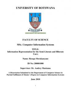
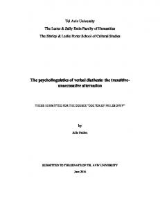
CHAPTER 4 : The Terra & Aqua Platforms The Terra Satellite: 4.5-billion-year history is a study in change. Natural geological forces have been rearranging the surface features and climatic conditions of our planet since its beginning. Today, there is compelling scientific evidence that human activities have attained the magnitude of a geological force and are speeding up the rates of global changes. For Figure 8: The TERRA Spacecraft example, carbon dioxide levels have risen 25 percent since the industrial revolution and about 40 percent of the world’s land surface has been transformed by humans. Launched in December 1999, Terra is the flagship of NASA's Earth Observing System (EOS) series of 10 satellites scheduled for launched over a 10-year period. EOS is part of NASA's Earth Science Enterprise, a longterm research program dedicated to understanding how human-induced and natural changes affect the global environment. The satellite was previously known as EOS AM-1, signifying its morning equatorial crossing time. The name Terra was given to the EOS AM-1 spacecraft by a 12th grader from St. Louis, Missouri in a contest that was co-sponsored by NASA and the American Geophysical Union (AGU). The satellite was manufactured by Lockheed Martin Missiles & Space (LMMS) and is managed by NASA's Goddard Space Flight Center. A multi-national mission, Terra carries a payload of five complementary sensors. The Clouds and the Earth's Radiant Energy System (CERES) and the Moderate-resolution Imaging Spectroradiometer (MODIS) instruments were developed by NASA Field Centers. The Measurements Of Pollution In The Troposphere (MOPITT) instrument was designed by Canadian scientists at the University of Toronto and manufactured by COM DEV International of Cambridge, Ontario. The Multi-angle Imaging SpectroRadiometer (MISR) instrument was built by Jet Propulsion Laboratory, while the Advanced Spaceborne Thermal Emission and Reflection Radiometer (ASTER) was developed in Japan for the Ministry of Economy Trade and Industry (METI).
22
On February 24, 2000, Terra began collecting what ultimately became a new, 15-year global data set on which to base scientific investigations about our complex home planet. Together with the entire fleet of EOS spacecraft, Terra is helping scientists unravel the mysteries of climate and environmental change. TERRA SATELLITE MISSION: On December 18,1999,NASA launched TERRA, its Earth Observing System (EOS) flagship satellite. In February 2000, Terra opened its Earthviewing doors to begin one of humanity’s largest and most ambitious science missions ever undertaken — to give Earth its first physical check-up. In particular, the mission is designed to improve understanding of the movements of carbon and energy throughout Earth’s climate System. Terra is a multi-national, multiFigure 9: NASA’s Terra Satellite disciplinary mission involving partnerships with the aerospace agencies of Canada and Japan. Managed by NASA’s Goddard Space Flight Center, the mission also receives key contributions from the Jet Propulsion Laboratory and Langley Research Center. Terra is an important part of NASA’s Science Mission, helping us better understand and protect our home planet. As it passed over Antarctica on December 16,2004, the Multi-angle Imaging SpectroRadiometer (MISR) on NASA’s Terra satellite captured this image showing a wavy pattern in a field of white. At most other latitudes, such wavy patterns would likely indicate clouds. MISR, however, saw something different. By using information from several of its multiple cameras (each of which looks at the Earth’s surface from a different angle), MISR was able to tell that what looked liked a wavy cloud pattern was actually a wavy pattern on the ice surface.In this image pair, the view from MISR’s most oblique (off-vertical) backward-viewing camera is on the left, while the color-coded image on the right shows the results of a computer program called a cloud mask, which uses MISR’s multi-angle, multi-spectral data to classify clouds and distinguish them from surface features. The colors represent the level of certainty with which the program made the 23
classification: white for areas that it labeled as cloud with high certainty (confidence), yellow for areas it labeled as cloud with less confidence; dark blue for areas it classified as clear with high confidence, light blue for areas it classified as clear with less confidence. MISR’s cloud mask works particularly well at detecting clouds over snow and ice, but also works over ocean and land.
Figure 10: (featured image) Waves on White: Ice or Clouds from Terra
The rippled area on the surface which could have been mistaken for clouds are actually sastrugi—long, wavelike ridges of snow formed by the wind and found on the polar plains. Usually sastrugi are only several centimeters high and several meters apart, but large portions of East Antarctica are covered by mega-sastrugi ice fields, with dune-like features as high as four meters. The mega-sastrugi result from unusual snow accumulation and redistribution processes that are influenced by the prevailing winds and climate conditions. The features provide information that is useful for icecore interpretation. MISR imagery indicates that these mega-sastrugi were stationary features between 2002 and 2004.
24
The five sensors onboard Terra are : • ASTER, or Advanced Spaceborne Thermal Emission and Reflection Radiometer; • CERES, or Clouds and Earth's Radiant Energy System; • MISR, or Multi-angle Imaging Spectroradiometer; • MODIS, or Moderate-resolution Imaging Spectroradiometer; and • MOPITT, or Measurements of Pollution in the Troposphere. The life expectancy of the EOS Terra mission is 6 years. It will be followed in later years by other EOS spacecraft that take advantage of new developments in remote sensing. The Aqua Satellite: Aqua, the twin sister satellite to NASA's Terra spacecraft, is the latest sibling in the Earth Observing System (EOS) series of satellites. Launched in May 2002, Aqua represents a multidisciplinary study of the world's global water cycle. Aqua was formerly named EOS PM, signifying its afternoon Figure 11: The AQUA Spacecraft equatorial crossing time. Aqua is an international partnership between the United States, Japan and Brazil. The spacecraft and four of Aqua's six scientific instruments are provided by NASA, while NASA's Goddard Space Flight Center provided the Moderate Resolution Imaging Spectroradiometer (MODIS) and the Advanced Microwave Sounding Unit (AMSU-A). Jet Propulsion Laboratory provided the Atmospheric Infrared Sounder (AIRS). NASA's Langley Research Center provided the Clouds and the Earth's Radiant Energy System (CERES) instrument. Japan's National Space Development Agency provided the Advanced Microwave Scanning Radiometer (AMSR-E). The Instituto Nacional de Pesquisas Espaciais (the Brazilian Institute for Space Research) provided the Humidity Sounder for Brazil (HSB). Instruments aboard Aqua employ the latest remote sensing technologies and take multiple readings of climate-related measurements, such as global precipitation, evaporation and the cycling of water, to 25
maximize the amount of information returned to Earth. Like Terra, Aqua instruments provide coverage on areas of largest uncertainty such as atmospheric humidity, radiative energy fluxes, aerosols, vegetation cover, phytoplankton and dissolved organic matter. Its Atmospheric Infrared Sounder (AIRS) instrument can help scientists to improve weather prediction and to observe changes in the climate. Scientists can better understand how global ecosystems are changing, how to respond to and affect global environmental change. In its first weeks of operation, after the instrument opened its Earth-view door, Aqua MODIS observed significant Earth events occurring all over the globe. MODIS collected and beamed to Earth images of typhoon, floods, and wildfires in 3 different areas in verynear real time. Japan's Advanced Microwave Scanning Radiometer (AMSRE) produced Aqua's first geophysical product: a global map of sea surface temperatures. Like Terra,the Aqua spacecraft is in a near-polar, sun synchronous orbit with an orbital period of 98.8 minutes. It has 6 years of mission life. Aqua provides direct broadcast services on X-Band. The spacecraft bus is scalable to meet the needs of future remote sensing missions, including Aura that is due to be launched in 2004. Aqua and subsequent EOS spacecraft due to be launched within the next decade will be operated in groups, rather than as single entities. Terra and Aqua are in formation with Landsat 7. This formation takes advantage of the enhanced calibration of Landsat's ETM+ instrument, which serves as an on-orbit standard for cross-calibration of other Earth remote sensing mission. AQUA SATELLITE MISSION: Aqua, Latin for water, is a NASA Earth Science satellite mission named for the large amount of information that the mission will Figure 12: NASA’s Aqua Satellite be collecting about the Earth's water cycle, including evaporation from the oceans, water vapor in the atmosphere, clouds, precipitation, soil moisture, sea ice, land ice, and snow cover on the land and ice. Additional variables also being measured by Aqua include radiative energy fluxes, aerosols, vegetation cover on the land, phytoplankton and dissolved organic matter in the oceans, and air, land, and water temperatures.
26
Aqua was launched on May 4, 2002, and has six Earth-observing instruments on board, collecting a variety of global data sets. Aqua was the first member launched of a group of satellites termed the Afternoon Constellation, or sometimes the A-Train. The second member to be launched was Aura, in July 2004, and the third member was PARASOL, in December 2004. Upcoming are CloudSat and CALIPSO in 2005 and OCO in the more distant future. Once completed, the A-Train will be led by OCO, followed by Aqua, then CloudSat, CALIPSO, PARASOL, and, in the rear, Aura. Source or Platform Program Management Aqua is part of NASA's Earth Science Enterprise, a long-term research effort dedicated to understanding and protecting Earth. Aqua is a joint project between the United States, Japan, and Brazil. Coverage Information Aqua flies in a sun-synchronous polar orbit with global coverage. Ground tracks repeat every 16 days or every 233 orbit revolutions. Path numbers are calculated based on the longitude of the orbital ascending node. With 233 paths, path 1 corresponds to 295.4 degrees east longitude. Since each orbit covers 16 grid lines, the path numbers increment by 16 for each orbit (NASA 2000).
April 11, 2005 Figure 13: (Featured Image) Phytoplankton bloom in the Gulf of Alaska from Aqua
27
The Aqua mission is a part of the NASA-centered international Earth Observing System (EOS). Aqua was formerly named EOS PM, signifying its afternoon equatorial crossing time. Attitude Characteristics • Inclination: 98 degrees • Altitude: 705 km • Period: 99 minutes • Semi-major axis: 7085 km • Eccentricity: 0.0015
28
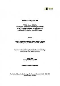
CHAPTER 5 :The MODIS Sensor MODIS (Moderate Resolution Imaging Spectroradiometer) is a key instrument aboard the Terra (EOS AM) and Aqua (EOS PM) satellites. Terra's orbit around the Earth is timed so that it passes from north to south across the equator in the morning, while Aqua passes south to north over the equator in the afternoon. Terra MODIS and Aqua MODIS are viewing the entire Earth's surface every 1 to 2 days, acquiring data in 36 spectral bands, or groups of wavelengths. These data will improve our understanding of global dynamics and processes occurring on the land, in the oceans, and in the lower atmosphere. MODIS is playing a vital role in the development of validated, global, interactive Earth system models able to predict global change accurately enough to assist policy makers in making sound decisions concerning the protection of our environment. The MODIS sensor flies onboard the Terra satellite platform launched by NASA in December 1999. In May 2002, NASA launched a second MODIS sensor on the Aqua mission. Both Terra and Aqua platforms have multiple sensors onboard and are part of a constellation of NASA satellites known as the Earth Observing System.
Figure 15: An Imaging Radiometer employing a cross track scan mirror,collecting Optics & a set of individual detector elements to provide imagery of the Earth’s surface & cloud cover in 36 discrete spectral bands.
29
The MODIS sensor is designed to monitor and provide integrated measurements of Earth's land, ocean and atmospheric processes. A particular phenomenon that MODIS is specifically designed to monitor is Fire. MODIS has several characteristics that facilitate its ability for daily global satellite fire detection. Each of the MODIS sensors has a field of view of 2,330 kilometers and orbits the Earth several times daily. With their field of view and orbit configuration, each MODIS sensor can view nearly the entire planet daily — once during the day and once nightly. As a result, the combination of both Modis sensors provide the opportunity to detect fire activity across the globe four times each day. MODIS also has a broad spectral resolution measuring reflected and emitted energy from the visible to thermal infrared wavelengths. These measurements are collected at one of three spatial resolutions: 250 meters, 500 meters and 1 kilometer. MODIS thermal image data are used to detect fire activity on both the daytime and nighttime observations. The fire detection locations resolved from MODIS thermal image data are compiled at a spatial resolution of 1 kilometer; however, in favorable conditions the sensor can identify fire activity covering just a fraction of the sampled 1 square kilometer area. With the launch of the Moderate Resolution Imaging Spectroradiometer (MODIS) in December 1999, a new era in hyperspectral satellite remote sensing began. MODIS makes possible continuous monitoring of the environment by measuring atmospheric trace gases and aerosol density, and mapping the surface of clouds, land and sea in a variety of spectral ranges from the blue to the thermal infra-red. The first Moderate Resolution Imaging Spectroradiometer (MODIS) sensor went into orbit with the launch of the TERRA (EOS AM-1) satellite on December 18, 1999. With the successful launch of AQUA (EOS PM-1) from Vandenberg Air Force Base, CA, on May 4, 2002, a second MODIS sensor was put into orbit for studying the Earth's water cycle and our environment. TERRA and AQUA (both with a 705km orbit) have a sunsynchronous, near polar, circular orbit. AQUA will cross the equator daily at 1:30 p.m. as it heads north (ascending mode) in contrast to TERRA, which crosses the equator at 10:30 a.m. daily (descending mode). With this formation it is expected that AQUA's afternoon observations combined with TERRA's morning observations will provide important insights into the daily cycling of global precipitation and ocean circulation.
30
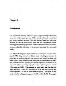
MODIS is a 36 band spectrometer providing a global data set every 1-2 days with a 16-day repeat cycle. The spatial resolution of MODIS (pixel size at nadir) is 250m for channel 1 and 2 (0.6µm - 0.9µm), 500m for channel 3 to 7 (0.4µm - 2.1µm) and 1000m for channel 8 to 36 (0.4µm 14.4µm), respectively. A detailed overview for the 36 spectral channels of MODIS is given in Table 1. The MODIS instrument consists of a cross-track scan mirror, collecting optics and individual detector elements. The swath dimensions of MODIS are 2330km (across track) by 10km (along track at nadir). The along track swath dimension is due to the optical set-up as well as the scanning mechanism of MODIS. In contrast to other scanning sensors like e.g. AVHRR, MODIS is observing within one scan ten lines of 1km spatial resolution (40 lines of 250m resolution and 20 lines of 500m resolution, respectively). Due to this unique feature, the so called panoramic "bow tie" -effect occurs at the border of each scene.
Figure 16: Three consecutive MODIS scans each consisting of ten 1 km lines. Due to the panoramic “bow tie “ effect, the scans are partially overlapping at off nadir angles. The first & third scans are represented by the light grey grids, while the second scan is shown in black.
In the above figure, a schematic layout of the "bow tie" effect is presented. All MODIS data are digitised in 12 bits. The real-time data stream carries the data from all 36 spectral bands for the entire MODIS field of view (2330km). The TERRA and AQUA platform have a sunsynchronous, near polar, circular orbit crossing the equator at 10:30 a.m. daily (descending mode for TERRA) and crossing the equator daily at 1:30 p.m. as it heads north (ascending mode for AQUA). Both satellites have a typical flight height of 705km.
31
MODIS Technical Specifications: Orbit:
705 km, 10:30 a.m. descending node (Terra) or 1:30 p.m. ascending node (Aqua), sun-synchronous, near-polar, circular
Scan Rate:
20.3 rpm, cross track
Swath Dimensions:
2330 km (cross track) by 10 km (along track at nadir)
Telescope:
17.78 cm diam. off-axis, afocal (collimated), with intermediate field stop
Size:
1.0 x 1.6 x 1.0 m
Weight:
228.7 kg
Power:
162.5 W (single orbit average)
Data Rate:
10.6 Mbps (peak daytime); 6.1 Mbps (orbital average)
Quantization: 12 bits Spatial Resolution:
250 m (bands 1-2) 500 m (bands 3-7) 1000 m (bands 8-36)
Design Life:
6 years
Table: Specification of the 36 MODIS channels, including primary use, central wavelength, bandwidth and spatial resolution. Primary Use
Band number
Central wavelength [nm]
Bandwidth [nm]
Spatial resolution [m]
Land / Cloud / Aerosols / Boundaries
1
645
620 - 670
250
2
858.5
841 - 876
Land / Cloud / Aerosols Properties
3
469
459 - 479
4
555
545 - 565
5
1240
1230 - 1250
6
1640
1628 - 1652
7
2130
2105 - 2155
8
421.5
405 - 420
9
443
438 - 448
10
488
483 - 493
Ocean Colour / Phytoplankton / Biogeochemistry
32
500
1000
Primary Use
Band number
Central wavelength [nm]
Bandwidth [nm]
11
531
526 – 536
12
551
546 – 556
13
667
662 – 672
14
678
673 – 683
15
748
743 – 753
16
869.5
862 – 877
17
905
890 – 920
18
936
931 – 941
19
940
915 – 965
20
3750
3660 – 3840
21
3959
3929 – 3989
22
3959
3929 – 3989
23
4050
4020 – 4080
Atmospheric Temperature
24
4465.5
4433 – 4498
25
4515.5
4482 – 4549
Cirrus Clouds / Water Vapour
26
1375
1360 – 1390
27
6715
6535 – 6895
28
7325
7175 – 7475
Cloud Properties
29
8550
8400 – 8700
Ozone
30
9730
9580 – 9880
Surface / Cloud Temperature
31
11030
10780 –11280
32
12020
11770 –12270
Cloud Top Altitude
33
13335
13185 –13485
34
13635
13485 –13785
35
13935
13785 –14085
36
14235
14085 –14385
Atmospheric Water Vapour
Surface / Cloud Temperature
33
Spatial resolution [m]
MODIS has a viewing swath width of 2,330 km and views the entire surface of the Earth every one to two days. Its detectors measure 36 spectral bands between 0.405 and 14.385 µm, and it acquires data at three spatial resolutions -- 250m, 500m, and 1,000m. Along with all the data from other instruments on board the Terra spacecraft, MODIS data are transferred to ground stations in White Sands, New Mexico, via the Tracking and Data Relay Satellite System (TDRSS). The data are then sent to the EOS Data and Operations System (EDOS) at the Goddard Space Flight Center. After Level 0 processing at EDOS, the Goddard Space Flight Center Earth Sciences Distributed Active Archive Center (GES DAAC) produces the Level 1A, Level 1B, geolocation and cloud mask products.
Figure 17: Typical daily coverage for the MODIS Direct Broadcast Receiving Station at Oberpfaffenhofen (DLR- DFD).
Higher-level products are produced by the MODIS Adaptive Processing System (MODAPS), and then are parceled out among three DAACs for distribution to various Organisations for different purposes. There are 44 standard MODIS data products that scientists are using to study global change. These products are being used by scientists from a variety of disciplines, including oceanography, biology, and atmospheric science. The MODIS instrument provides high radiometric sensitivity (12 bit) in 36 spectral bands ranging in wavelength from 0.4 µm to 14.4 µm. The responses are custom tailored to the individual needs of the user community and provide exceptionally low out-of-band response. Two bands are imaged at a nominal resolution of 250 m at nadir, with five bands at 500 m, and the remaining 29 bands at 1 km. A ±55-degree scanning pattern at the EOS orbit of 705 km achieves a 2,330-km swath and provides global coverage every one to two days. 34
The Scan Mirror Assembly uses a continuously rotating double-sided scan mirror to scan ±55-degrees and is driven by a motor encoder built to operate at 100 percent duty cycle throughout the 6-year instrument design life. The optical system consists of a two-mirror off-axis afocal telescope, which directs energy to four refractive objective assemblies; one for each of the VIS, NIR, SWIR/MWIR and LWIR spectral regions to cover a total spectral range of 0.4 to 14.4 µm. A high-performance passive radiative cooler provides cooling to 83K for the 20 infrared spectral bands on two HgCdTe Focal Plane Assemblies (FPAs). Novel photodiode-silicon readout technology for the visible and near infrared provide unsurpassed quantum efficiency and low-noise readout with exceptional dynamic range.
Figure 18: The MODIS Sensor
Analog programmable gain and offset and FPA clock and bias electronics are located near the FPAs in two dedicated electronics modules, the Space-viewing Analog Module (SAM) and the Forward-viewing Analog Module (FAM) . A third module, the Main Electronics Module (MEM) provides power, control systems, command and telemetry, and calibration electronics. The system also includes four on-board calibrators as well as a view to space: a Solar Diffuser (SD), a v-groove Blackbody (BB), a Spectroradiometric calibration assembly (SRCA), and a Solar Diffuser StabilityMonitor,(SDSM). 35
The first MODIS Flight Instrument, ProtoFlight Model or PFM, was integrated on the Terra (EOS AM-1) spacecraft. Terra successfully launched on December 18, 1999. The second MODIS flight instrument, Flight Model 1 or FM1, was also integrated on the Aqua (EOS PM-1) spacecraft; it was successfully launched on May 4, 2002. These MODIS instruments offer an unprecedented look at terrestrial, atmospheric, and ocean phenomenology for a wide and diverse community of users throughout the world.
36
CHAPTER- 6 : MODIS PRODUCTS There are different standard satellite products over Land, Atmosphere and ocean giving different geophysical parameters over local, regional and global scales. These products are available on daily, weekly and monthly basis. 1) Land Global change research investigates the underlying processes of change and their manifestation, the impacts and the prediction of change. Monitoring these changes provides an important underpinning to both global change research and resource management. Monitoring of land cover and land use is an important element of the NASA Earth Science Enterprise. Moderate resolution remote sensing provides a means for quantifying land surface characteristics such as land cover type and extent, snow cover extent, surface temperature, leaf area index, fire occurrence. Satellite measurements of leaf area, leaf duration and net primary productivity provide important inputs to parameterize or validate ecosystem process models. High quality, consistent and well-calibrated satellite measurements are needed if we are to detect and monitor changes and trends in these variables. Developing the next-generation data sets for global change research is the challenge given to the MODIS Science Team. 2) Atmosphere One of the most important ecological issues concerning our planet is climate change. It is generally agreed that the Earth's climate will modify in response to radiative forcing induced by changes in atmospheric trace gases, cloud cover, cloud type, solar radiation, and tropospheric aerosols (liquid or solid particles suspended in the air). In order to develop conceptual and predictive global climate models, it is vital to monitor these properties. Two MODIS (Moderate Resolution Imaging Spectroradiometer) instruments, the first launched on 18 December 1999 onboard the Terra Platform and the second on 4 May 2002 onboard the Aqua platform, are uniquely designed (wide spectral range, high spatial resolution, and near daily global coverage) to observe and monitor these and other Earth changes. 3) Ocean 4) Calibration 5) Cyrosphere
37
DATA PRODUCTS MODIS (Terra and Aqua) satellite products are available for different geophysical parameters which are used under Land, Ocean & Atmospheric applications. The MODIS instruments on the Terra and Aqua platforms provide measurements on a global basis every 1-2 days with a 16-day repeat cycle. A list of the 44 MODIS data products are given below : Data Product Name
Data Code
Level 1A Radiance Counts
MOD 01
Level 1B Calibrated, Geolocated Radiances
MOD 02
Geolocation Data Set
MOD 03
Aerosol Product
MOD 04
Total Precipitable Water (near-IR method)
MOD 05
Cloud Products (optical thickness, particle radius, etc)
MOD 06
Cloud Products (cloud top properties and phase)
MOD 06
Atmospheric Profiles
MOD 07
Gridded Atmosphere Products-Level 3
MOD 08
Atmospherically Corrected Surface Reflectance
MOD 09
Snowcover
MOD 10
Land Surface Temperature and Emissivity
MOD 11
Land Cover/Land Cover Change
MOD 12
Vegetation Indices
MOD 13
Thermal Anomalies, Fires, Biomass Burning
MOD 14
Leaf Area Index and FPAR
MOD 15
Surface Resistance and Evapotranspiration
MOD 16
Vegetation Production , Net Primary Productivity
MOD 17
Normalized Water Leaving Radiance
MOD 18
Pigment Concentration
MOD 19
38
Data Product Name
Data Code
Chlorophyll II Fluorescence
MOD 20
Chlorophyll a Pigment Concentration
MOD 21
Photosynthetically Active Radiation (PAR)
MOD 22
Suspended Solids Concentration in Ocean Water
MOD 23
Organic Matter Concentration
MOD 24
Coccolith Concentration
MOD 25
Ocean Water Attenuation Coefficient
MOD 26
Ocean Primary Productivity
MOD 27
Sea Surface Temperature
MOD 28
Sea Ice Cover
MOD 29
Temperature and Moisture Profiles
MOD 30
Phycoerythrin Concentration
MOD 31
Ocean Processing Framework and Matchup DB
MOD 32
Gridded Snowcover
MOD 33
Gridded Vegetation Indices
MOD 34
Cloud Mask
MOD 35
Total Absorption Coefficient
MOD 36
Ocean Aerosol Properties
MOD 37
Clear Water Epsilon
MOD 39
Albedo 16-Day Level 3
MOD 43
Vegetaion Cover Conversion and Continuous Fields
MOD 44
The Modis products are categorized at different levels of their applications as: a) MODIS Level 1A and Level 1B data products : Calibrated radiance and geolocation and onboard calibration/engineering data. b) MODIS Level 2 data products c) MODIS Level 3 data products d) MODIS Level 4 data products
39
Considering Atmospheric application and concentrating on Atmospheric aerosols and its related studies, some of the Atmospheric products were considered for study. Out of Aerosol, Cloud, Water vapor and Ozone products, only Aerosol concentration and Water vapour were considered. These data products are available on daily, weekly and monthly composite products and are available and downloadable from the MODIS website.
THE STUDY AREA The Aerosol Products were considered from March to June 2005,in and around Dehradun area between the coordinates 30o17’ to 30o31’ N and 78o30’ to 78o13’ E. It is bounded by a part of Dehradun district in the north, Haridwar district in the south, Siwalik ridges in the west and Pauri Garhwal and Tehri Garhwal in the east. The study area comes under the administrative boundaries of Dehradun district, Uttaranchal State. PHYSIOLOGY The study area consists of both hilly and plain terrain. Song and Jakhan rivers, flowing on its eastern and western part respectively drain it. These two main rivers provide the drainage pattern of the study area by dividing into a number of raus and streams,especially in the western and parts of the study area. The raus carry immense volume of water, boulder ond loose shingles their beds during monsoon. They have very wide and shallow beds and remain dry during most parts of the year. SOIL The soils in the study area exhibit wide variation due to their texture, depth, stoniness, color, drainage, moisture, organic matter, carbon exchange, etc. CLIMATE The climate of the area varies from sub-tropical type to temperate depending upon the altitude . There are three distinct seasons of Monsoon, winter and summer periods. The hottest months are May and June and the coolest months are December, January and February. The main annual temperatures of summer and winter are 38.2oC and 3oC respectively. Heavy rainfall occurs during the monsoon and small amounts of rainfall is also received during January and February. The area receives an average annual rainfall of 2073.3mm (Anon). Prevailing wind direction is westward and is of moderate velocity. Occasional thunderstorms are seen after February. 40
Frost is common in winter nights, being severe in the months of January and February. Night dews prevail uninterrupted throughout the year except from April to May and part of June. Data Images
Aerosol optical thickness at 0.55 microns for both Ocean and land : Mean of daily mean. (1st to 9th May 2005).
Average optical thickness at seven bands for average solution : Mean of daily Mean (B3) (1-9 May, 2005)
41
Water vapor near IR – clear column: Mean of daily mean (1-9 May, 2005)
Total column precipitable water vapor – IR retrevial : Mean of daily mean (1-9 May,2005)
42
Daily data small mode Aerosol fraction Over Dehradun area (TERRA) as on 6th June, 2005
Total column Precipitable Water Vapor IR ,Dehradun as on 6th June, 2005
Total column precipitable Water Vapor near IR (7th April,Terra ).
43
The sample products for the weekly as well as daily for aerosol parameters were studied. The weekly product were of global nature and daily were for the Dehradun area. For many dates the data was not good hence the sample data for good days was taken. These are just samples of the standard weekly global products of the geophysical parameters. There are other parameters that are given alongwith these data. These parameters are used for further research studies.
ANALYSIS AND CONCLUSION : Dehradun area is largely surrounded by forests and highly vegetated. The mining activities are also in and around Dehradun due to its richness in Calcium, hence the study of aerosols and its related parameters holds an important research area over this region. Aerosols leads to the formation of local clouds, dust, fog etc. which is major during winters. Hence, the study the different parameters of Aerosols could help in explaining the transport as well as explaining the physical and optical properties and long trend helps in understanding the characteristics of Aerosols.
44
REFERENCES
1. Fundamentals of Remote Sensing By
G eorge Joseph
By
A ndrew D avid
By
D eepak
By
Fym atA lain
2. An introduction to Atmospheric physics
3. Remote Sensing of Atmosphere and Oceans
Adarsh 4. Remote Sensing of Atmosphere
5. MODIS website http://modis.gsfc.nasa.gov/ 6. MODIS Atmosphere website http://modis-atmos.gsfc.nasa.gov/ 7. Earth Observing Station Data Gateway http://edcimswww.cr.usgs.gov/pub/imswelcome/ 8. Online Data sets http://daac.gsfc.nasa.gov/data/datapool/ 9. Earth Science Data interface http://glcfapp.umiacs.umd.edu:8080/esdi/index.jsp
45