development, therefore, has the most crucial role in a child's intellectual
development. The family is ... The need for money for productive activities, such
as investment in human capital, has to compete with .... Organization of the
Dissertation.
Chapter I INTRODUCTION
Investment in human capital plays an important role in a country’s economic development. By examining data from 98 countries in the period 1960-1985, Barro (1991) found a positive relationship between initial human capital and the growth rate of real per capita Gross Domestic Product (GDP). This means that when all other factors are controlled, countries with higher human capital may have higher economic growth. Higher human capital can basically determine a nation’s productivity which is considered a very important source of economic growth besides the expansion of inputs. Numerous quantitative studies of the sources of economic growth in the West have demonstrated that the growth of human capital has been the principal source of economic growth (Todaro, 1985). The outstanding experiences of fast growing Asian economies such as Taiwan, Hong Kong, and South Korea are perhaps obvious examples of the importance of human capital to economic growth. Despite the lack of natural resources, these countries have managed to grow faster than any other countries, because they have had higher quality in human capital (Becker, 1992). Economists and other social scientists have applied the concept of human capital since the 1950’s in many ways (Bryant, 1990). Schultz (1972), who is considered a pioneer in human capital theory, classified investment in human capital into investment in (1) schooling and higher education, (2) post-school training and learning, (3) pre-school learning activities, (4) migration, (5) health, (6) information, and (7) investment in children. Hence, the concept of human capital has been used in a wide variety of ways. Becker (1975), for example, in his book Human Capital discussed investment in human capital in the context of the labor market. Investment in human capital also could be discussed in relation to changes in fertility decisions and mortality (Becker, 1992). The family, as an economic organization unit in society, has a very important role in investment in human capital, particularly investment in children. The family should
1
make the decision of investment, whether in human capital, i.e., in children, or in other assets.
Their decision making processes underlie all functions of family resource
management (Deacon & Firebaugh, 1981). Family economists, therefore, could apply the concept of human capital in the context of family resource management. Recent studies show that the period from birth to 3 years old is very crucial for a child’s development (Santrock, 1998). Blakeslee (1997) reported that child development scientists presented their important findings in the White House conference on early child development. One interesting finding indicated that a child’s neurological foundation for cognitive abilities such as rational thinking, problem solving and general reasoning appears to be largely developed by age one. Spoken language was shown to be important in an infant’s brain development. In fact, some researchers stated that the number of words an infant hears each day is the single most important predictor of later intelligence, school success, and social competence.
These findings show how important early child
development is in determining the later cognitive ability, hence the quality of human capital. The family, as a major environment for children during the early years of development, therefore, has the most crucial role in a child’s intellectual development. The family is responsible for conducting the activities of early childhood education which prepare children for further educational processes (Zeitlin, Kramer, & Megawangi, 1992). Parents are expected to provide a stimulating environment that spurs children’s mental and physical development.
Family and Human Capital in Indonesia
In 1996, according to Badan Koordinasi Keluarga Berencana Nasional (the National Family Planning Coordinating Board), it was estimated that about 23.4 % and 24.8 % of Indonesian families were classified as pre-prosperous families and first degree prosperous families, respectively (BKKBN, 1997). Pre-prosperous families are those who
2
have not yet been able to meet their basic needs. First degree prosperous families are those who have already met their basic needs minimally but they have not yet been able to meet their socio-psychological needs. Families in these two categories are considered to be families who live in poverty. This means that about 50 % of families in Indonesia live in poverty. There are several factors identified as the cause of poverty in the family. These factors, according to BKKBN (1997), can be categorized into internal and external factors. Internal factors that contribute to poverty are morbidity, lower education, lack of knowledge, skills, and monetary capital, and the fact of having fallen behind in technology. External factors such as socio-economic structure, culture, and less access to economic and health facilities also may contribute to family poverty. The 1993 Indonesian Guidelines of State Policy (GBHN) state the development policy of the prosperous family. This policy is an integral part of population policy which directs the development of the Indonesian people and the entire society to achieve happiness and a prosperous life. The importance of the family in the context of national development in Indonesia also is reflected by the promulgation of government bill No. 21/1994 which addresses the implementation of the development of the prosperous family. According to the bill, the family should perform eight functions which are: (1) religious, (2) socio-cultural, (3) sharing of love, including the process of democratization in the family, (4) the family as sanctuary for the individual member, (5) reproduction, (6) socialization, (7) production, and (8) environmental protection. A prosperous family should be able to perform these eight functions well, and the government implemented policies and programs to help the family to perform these functions. This is recognition of the importance of the family to the course of a national development program in general, particularly to the improvement of the quality of life. In Indonesia, the level of education, one indicator of the quality of human capital, has improved substantially. In the past two decades, education of those 10 years of age and over has increased markedly.
Enrollment rates in all levels of education have
3
improved for both males and females. In addition, the illiteracy rate has declined. In 1993, the illiteracy rates of rural and urban populations were about 18 percent and 7 percent, respectively (Central Bureau of Statistics, 1995). The illiteracy rate has improved from about 50 percent in both urban and rural populations in 1971. The infant mortality rate has decreased from 90 per 1,000 live births in 1980 to 53 per 1,000 live births in 1994 (World Bank, 1996). This phenomenon indicates that community health and nutritional status have improved. As a result of the declining mortality rate, the life expectancy has increased from 46 years in 1971 to 63 years in 1994. The decreasing mortality rate and the increasing life expectancy are other signs of the improvement of the quality of human capital in Indonesia. The improvement of the quality of human capital is often attributed to the development program. The substantial progress in education, for example, is due to a compulsory education program at the elementary and middle school levels. The decrease in the infant mortality rate is attributed to health programs which provide health infrastructure and personnel. The role of the family in achieving those improvements seems to be overlooked. This happens because very limited studies have been conducted to analyze the role of family in the improvement of the quality of human capital. This study was designed to contribute to the theoretical and empirical knowledge about the importance of the family in the improvement of human capital, particularly families’ behavior in allocating their resources to improve the quality of children. The focus of this study will be on the allocation of family income and parent’s time for activities that spur children’s intellectual development. Money (income) and parent’s time are two important resources that need to be well managed and utilized to achieve family goals. The need for money for productive activities, such as investment in human capital, has to compete with the need for consumption activities. Also, the need for time for parenting and child care has to compete with the need for working in the labor market. This situation leads parents to make decisions about their resource allocation.
4
Purposes and Objectives of the Study
In general, this study was intended to learn about family behavior concerning their allocation of resources to improve the quality of their children and to investigate the factors that influence family behavior on investing in children in rural families in Indonesia. The specific objectives of this study were: 1. To determine the time allocation for activities that may stimulate the child’s growth and development which is called parental time investment. 2. To determine the income allocation for expenses that may have the effect of increasing the quality of a child which is called parental monetary investment. 3. To identify factors that influence parental time investment and parental monetary investment to enhance the quality of children. 4. To determine the relationship between parental time investment and parental monetary investment in children. 5. To determine the impact of parental time investment and parental monetary investment on the quality of children. The results of this study may give public policy makers and other researchers an understanding of rural family behavior on investing in children. By better understanding this matter, public policy makers will be able to formulate suitable intervention policies which can be directed to the family to enhance the quality of human capital and to alleviate poverty. Researchers who are interested in the study of family investment in children are expected to get more information, so they will be able to conduct in-depth study and further investigation.
Problem Statement and Research Questions
The development of a prosperous family is parallel to a poverty alleviation program. Both programs have the same ultimate goal which is to improve the quality of
5
life.
Therefore, the prosperous family development program has been linked to the
poverty alleviation program. In recent years, the government has launched a program called KUKESRA (Kredit Usaha Keluarga Sejahtera -- an Indonesian acronym). The program is basically to provide the family with a low interest loan to start a small business and income generating activities. By providing the family with a loan, it is expected that women in the family will be able to do productive activities and contribute to the family income. This program may have a positive effect on family income. On the other hand, it may encourage women in the family to work outside the home which will reduce the time spent with children. In Indonesia, women (mothers) are still perceived to be the main person in the family with responsibility for child care. Guhardja, Hartoyo, Megawangi, Sumarwan, and Heryatno (1995) found that 90% of families reported that mothers are the primary caretakers of children.
The other primary caretakers of children are fathers (3.5%),
grandmothers (2.8%), other relatives (1.7%), older brothers/sisters (1%), and maids (1%). A commercial child care service has not yet become a part of rural family life for many reasons. These facts indicate the importance of women in child rearing activities at home. If women (mothers) are encouraged to work outside the home, it might influence the child rearing practices, and in turn, might have a negative impact on child quality since they may spend less time with children or may stop doing some things with children which affect child quality. The present study addressed the main research question: What is the relative importance of parental monetary investment and parental time investment on the quality of children in rural Javanese and Minangese families?
It also addressed specific research
questions, as follows: 1. “How much time do mothers in rural areas spend daily for feeding the child and playing with the child as an indicator of parental time investment?” 2. “How much per capita expenditure do families in rural areas spend for food, education, and health care as an indicator of parental monetary investment?”
6
3. “What variables contribute to the differences in parental time investment?” 4. “What variables contribute to the difference in parental monetary investment?” 5. “What is the relationship between parental time investment and parental monetary investment? Is there a trade-off relationship between these two variables of investment in children?” 6. “How do parental time investment and parental monetary investment affect the child’s nutritional status and the child’s intellectual ability?”
Delimitations of the Study
The utilization of a pre-existing database delimited the researcher in terms of the conceptualization of variables and the scope of research. The examined variables and research questions of the study were necessarily constrained by the information provided in the database. The examined variables which are expected to affect parental investment in children and child quality were delimited to family expenditure, mother’s and father’s education, mother’s occupation, family size, family type, number of school-age children, child’s age, child’s gender, and ethnic group. This study also was delimited to nutritional status and IQ score of an observed child in each family sample as indicators of child quality. The ethnic group was delimited to two ethnic groups: Javanese and Minangese. Mother’s and father’s education were delimited to formal education. Examination of variables affecting child quality was delimited to include the sample whose children completed the IQ test and had anthropometric data (age and weight). Because of many reasons, some of children failed to take a complete IQ test or did not have anthropometric data.
7
Limitations of the Study
The database used for this study was designed for other purposes and covered rural families in two different ethnic groups, therefore it limits the generalizability of the findings. For example, samples were drawn from rural families in the Wonogiri and Agam districts. They may not represent all Indonesian rural families since there are many other ethnic groups in Indonesia. They also might not represent the Javanese or the Minangese population, as there are a variety of dialects within these two ethnic groups. The measure of per capita expenditure for food, education, and health care as an indicator of parental monetary investment in children was a limitation of the study. Total expenditure devoted to children may be a more appropriate measure of parental monetary investment. The measure of parental time investment in children was limited to mother’s time spent feeding and playing with the child. Total time devoted by parents and other family members to the child in any kind of activities that stimulate physical and cognitive development may be a more appropriate measure of parental time investment in children. There may be some misinterpretation of the questionnaires, memory error, inaccuracy in measuring, recalling, and reporting the daily activities and the length of each activity as well as the income allocation.
Conceptual Definition of Terms
Explanation of the definition of terms used in this study is intended to facilitate an understanding of their uses in further analysis, interpretation and discussion of the findings. The conceptual definitions of terms are: Human capital.
Human capital is all aspects that humans possess, including the
knowledge, skills, abilities, and attitudes that enable them to function in society and to produce needed goods and services.
8
Investment in children. Investment in children is all efforts, activities, or allocation of family resources that are intended to increase the quality of children who are expected to mature into productive citizens. The study focused on two ways of investing in children: monetary and time investments. The quality of children.
The quality of children indicates the physical growth and
intellectual capacity of children which may determine later productivity. Parental time investment. Parental time investment refers to the amount of time spent by the parent, particularly the mother, on activities that may stimulate and increase children’s physical growth and intellectual development. Parental monetary investment. Parental monetary investment refers to the amount of money allocated by the family to food, education, and health care that may determine the quality of children.
Organization of the Dissertation
This chapter provides an overview of the importance of human capital to economic development and the important role of the family in investment in human capital. The problem statements and the purpose of the study were outlined. This chapter presents the limitations and delimitations and the conceptual definition of terms used for the purpose of the study. The organization of the remaining chapters are as follows: Chapter II, Review of Literature; Chapter III, Theoretical and Empirical Model of Family Investment in Children; Chapter IV, Methodology; Chapter V, Findings and Discussions; and Chapter VI, Summary, Conclusions, and Recommendations.
9
Chapter II REVIEW OF LITERATURE
This chapter will briefly review theoretical or empirical works in human capital and family economics that are closely related to this study. This chapter will be divided into four sections. The first section will discuss cultural backgrounds, family relations, and value of children in Indonesian perspectives. The second section will provide an overview of the role of the family in human capital development. The third section will examine the literature concerning family resource allocation, particularly for investment activities in children. The discussion of the third section will be focused on the income allocation for education and health, the parent’s time allocation for child care, and factors related to income and time allocation. The fourth section will discuss and examine empirical studies that have been conducted on the topics of investment in children and household production.
Cultural Background and Value of Children
Indonesia is considered to be a culturally diverse nation. There are about 36 major ethnic groups in Indonesia of which the Javanese is the largest ethnic group (Megawangi, 1997). Hugo, Hull, Hull, and Jones (1987) used language to approximate Javanese dominance and found that about 40% of Indonesians speak Javanese at home. Most Javanese live on Java Island. It is estimated that 58% of those who live on Java Island are expected to be Javanese since they speak Javanese. According to the Central Bureau of Statistics (1996) it was estimated that about 60% of the Indonesian population (114 million people) live on Java Island. It is difficult, therefore, to speak about general Indonesian culture due to the diversity in ethnic groups. Each ethnic group may have a different culture. However, today social acculturation may be difficult to prevent because of the population migration and mobility.
10
Cultural background may influence family norms and daily habits. In terms of childrearing, mothers are perceived to be the primary caretakers of children. A study conducted with Javanese (Central Java) and Minangese (West Sumatera) indicates that 90% of families perceive mothers to be responsible for child care and there is no difference in this perception between Javanese and Minangese (Guhardja et al., 1995). Substitute child caretakers were grandmothers (37.8%), fathers (27.2%), older brothers/sisters (22.6%), relatives (8.1%), and neighbours (3.2%).
More Javanese fathers and
grandmothers were involved as substitute child caretakers than were the Minangese, while more Minangese older brothers/sisters were involved in child care activities than were the Javanese. A greater difference in the role of fathers (husbands) also occurs between Javanese and Minahasan (North Sulawesi) families. Megawangi, Sumarwan, Hartoyo, and Karsin (1994) reported that husbands in Javanese families are more involved in household work, in general. On the average, Javanese husbands spend 2.5 hours on housework and 1.4 hours per day on child care, compared to less than one hour for both activities in Minahasan families. The difference in husbands’ involvement in housework and child care may be caused by cultural and social backgrounds. Mulder (1978) stated that rukun (an Indonesian word which is originally from the Javanese language which means harmonious unity) is considered to be the most ideal social-relationship among Indonesian people, notably the Javanese. The concept of rukun is also applied in marriage relationships.
According to Koentjaraningrat (1985), the
equality of men and women and that of husband and wife are recognized normatively among the Javanese and the Javanese believe that husbands and wives should work together. Goodnow and Bowes (1994) pointed out that equality between husbands and wives may lead them to share household work. Javanese tend to have a bilateral kinship system which means children can follow either their father’s or their mother’s heritage. Minangese are considered to have a matriarchial kinship system which is characterized by women’s domination in the house
11
and descent is considered to be through the mother’s line. Sato (1982) observed that in the traditional Minangese society, the position of a male is a strange one in a modern society. He does not own any property, although he may manage and expand it for his sisters and their children. Children are perceived by most Indonesians to be the source of family joy and happiness (Koentjaraningrat, 1985; Geertz, 1961). According to Geertz (1961), for the Javanese having children brings luck and happiness and it makes warmth in the family, and calm and peace in the heart of parents. Based on a collaborative study conducted in 1986 by the Ministry of Population and Environment and the Demography Institute of the University of Indonesia in Jakarta and Surabaya, families perceive children to have more psychological than merely economical value (Megawangi, 1997). More than 90% of families in the study agree that children have such psychological values as: strengthening the marriage bond, being a sacred goal of the marriage, completion of womanhood and of manhood, and the source of joy and happiness. Meanwhile the percentage who agree with the statement that “children can provide security in old age” was only about 70%. Megawangi (1997) stated that a shift in parent’s perception of the economic value of children may occur in Indonesian society. In the most current study conducted by Megawangi et. al. (1994) in East Java, the percentage who agreed with the statement that “children can provide security at old age” was only 53%. It means that fewer parents depend on children for their security in old age. This shifting might have a relevancy with the development of the social security system. Nowadays, it is relatively easy to get services from bank, insurance, or investment companies. Therefore parents may have alternative ways to invest their money in financial institutions for their old age. Preference for the sex of children in Indonesian society is relatively equal. It means that both sexes are equally preferred by parents. Singarimbun, Darroch, and Meyer (1977) showed that the ideal number of children that parents prefer is four, consisting of two boys and two girls. The ideal number of children seems to be declining. Based on the 1991 Indonesia Demographic and Health Survey, about 57% of ever-married and
12
currently married women in the sample perceived the ideal number of children to be three or less. The study also found that the differences in the mean ideal number of children between regions and provinces was substantial, ranging from 2.4 children in Bali to 4.5 children in Aceh. The mean ideal number of children in the Java-Bali islands was reported to be lower than that in Outer Java-Bali islands. One factor that causes the difference in the mean ideal number of children across the regions and provinces is the degree of exposure to family planning programs. One of the activities of the family planning program is the campaign to institutionalize the smaller family norm with the slogan “two children are enough, boys and girls are the same, it does not matter.” Java-Bali islands are the main and initial target of the program since about 60% of the population lives in these islands. Supported by relatively good infrastructures, families in the Java-Bali islands are more likely to be influenced by the family planning program, particularly by the slogan campaign. This may change their perspective on the ideally desired number of children and, in turn, make families adopt contraceptive use. The prevalence of contraceptive use is the highest in Java-Bali islands. Having fewer children in the family may influence the allocation of family resources to children. The number of children in the family does affect the investment in children, particularly during the time when resources are scarce. With fewer children, parents may be able to distribute more resources to each child. This may affect child quality since each child is provided with more resources.
Family and Human Capital Development
Scientists have defined the family in many ways depending on their background and the context in which the definitions are being used. The family is studied not only by family studies experts but also by experts from other disciplines, such as economics, sociology, and psychology.
The family, according to Mattessich and Hill (1987), is
13
defined as a group in which its members relate to each other by kinship, residence, or close emotional attachment and display four systemic features: intimate interdependence, selective boundary maintenance, ability to adapt to change and maintain their identity over time, and performance of family tasks. This definition seems to be more flexible and to accommodate a wide variety of family forms. Furthermore, they mention that the family performs such tasks as: physical maintenance, socialization and education, control of social and sexual behavior, maintenance of family morale and of motivation to perform roles inside and outside the family, the acquisition of mature family members by the formation of sexual partnerships, the acquisition of new family members through procreation or adoption, and the launching of juvenile members from the family when mature (Mattessich & Hill, 1987). In other words, the family is basically the place where all members (including children) receive a foothold in life. The family is responsible for the maintenance and development of family members (Deacon & Firebaugh, 1981).
In order to be able to perform the maintenance and
development of family members, families must foster and direct their children’s development through such functions as: (1) parental nurturing, (2) personality integration, (3) socialization, and (4) enculturation (Lidz, 1981). The parental nurturant function means that the family must provide for the child’s physical needs as well as his/her emotional needs for love and affection, and a sense of security, so that he/she will be able to grow and develop to be a mature person. Personality integration, socialization, and enculturation functions are intended to make the children able to develop and to function in the ways the society wants when they emerge from the family. As the source of human resources, the family is expected to perform those functions well, so they will produce good human capital. However, for many reasons, some families do not perform the functions as expected. As a consequence, the family is not only the source of human resources, but also the source of emotional incapacity (Lidz, 1981) which may decrease the quality of human capital. For example, a disorganized, low
14
income family may produce a delinquent child (Minuchin, Montalvo, Guerney, Rosmau, & Schumer, 1967). The early childhood stage of development is believed to be a very important and crucial stage for children. Recent studies indicate that the neurological foundation for rational thinking, problem solving, and general reasoning appears to be largely established by age one (Blakeslee, 1997; Santrock, 1998; Cole & Cole, 1993) and half of a person’s intelligence potential is developed by age four (Bloom, 1964). During the early childhood years, children may have interaction primarily with family. This makes the family very important for children’s development. Leibowitz (1974) noted that the significant differences in verbal and mathematical competence of children who enter first grade reflected the variation in (1) inherent ability and (2) the amount of human capital acquired before the children reach age six. The amount of human capital acquired reflects the various efforts that have been conducted by the family in relation to the quality of human capital.
Furthermore, she described two
types of input which were considered as home investment: time input and goods input. Family investment in human capital could be considered as consumption as well as household production. When a family spends income for education and health services, the spending may be considered as consumption, because they directly satisfy family wants. Meanwhile, when a family spends its time for child care or other activities that stimulate the child’s intellectual development, their acitivities may be considered as household production. Both activities, however, are classified as investment in human capital, since both are considered as resource reallocation for future consumption and production. Investment in human capital by a family can take many different forms, such as: formal schooling, on the job training and experience, and maintenance and augmentation of health (Bryant, 1990). A more specific classification of investment in human capital activities was developed by Schultz (1972). The seven different activities of investment in human capital classified were: (1) schooling and higher education, (2) postschool training
15
and learning, (3) preschool learning activities, (4) migration, (5) health, (6) information, and (7) investment in children (population).
Allocation of Family Resources for Human Capital Investment
The family usually has multiple goals, including the goal concerning human capital. The family deals with relatively limited resources and sometimes does not have complete control of the resources. This situation leads the family to use management to achieve family goals (Gross, Crandall, & Knoll, 1980; Deacon & Firebaugh, 1981; Goldsmith, 1996). Management helps the family utilize limited resources effectively and efficiently to achieve the family goals. In relation to human capital development, the family should allocate its resources to make all family members better people and to have the quality they expect. Children’s continual development as healthy, happy, and competent individuals is the concern of parents (Kuzma, 1980). The two important family resources that can be used to achieve the goal related to children’s development are: time and income. When family resources become more limited relative to the need for resources, the use of resources for human capital competes with the need for resources for other family goals. For example, as more mothers engage in the labor market, mothers’ time available for household work, particularly for child care, becomes smaller.
Income Allocation for Food, Health, and Education
Family efforts in investment in children could be reflected in the allocation of income and time. Parents who are aware of the quality of children may spend more money and more time for the activities or needs that increase the quality of children. Based on the 1993 U.S. Consumer Expenditure Survey (CES) data, on the average, expenditure shares for food (at home and away from home), health care, and education were 14.0
16
percent, 5.2 percent, and 1.4 percent, respectively (Anonymous, 1996). Compared to 1984, the expenditure share of food has decreased from 15.0 percent, while the shares of health care and of education have increased from 4.7 percent and 1.3 percent, respectively. The increasing shares of health care and of education could be attributed to increasing price (Anonymous, 1996). According to Maksum (1997) of the Central Bureau of Statistics, in Indonesia, the average expenditure share of food in 1993 was about 56.9 percent, while expenditure shares of health care and of education were about 1.3 percent and 2.9 percent, respectively. As a developing and lower middle-income country, it is understandable that the share of food still accounted for the largest part of the expenditure, while the shares of health care and education were very small. As income has increased, the expenditure share of food, however, has decreased from 63.2 percent in 1984. Maksum (1997) also reports that data from the 1993 and 1996 National SocioEconomic Surveys indicate that the expenditure shares of health care and education increased.
In 1993, on average, Indonesians spent about 1.3 percent of the total
expenditure for health care services and 2.9 percent for education.
In 1996, the
expenditure shares of health care and education increased, respectively, to 1.7 percent and 3.0 percent of the total expenditure. Contrary to what happens in the U.S., in Indonesia, expense for education is higher than for health care. This might be because in Indonesia the relative price of education on the aggregate tends to be higher than the price of health care services, as compared to the U.S. For some Indonesians, particularly those who live in rural and remote areas, traditional, low-cost health care methods remain the major methods to overcome health problems. Meanwhile, for education, even though there is no tuition fee for elementary school students, parents are still obligated to pay some other education-related expenses, e.g., books, uniform, and allowances. Abdel-Ghany and Foster (1982) found that income elasticities for health care and for education are 1.11 and 1.03, respectively, while for food it is 0.48. It means that if the income increases by one percent, income allocation for health care and for education
17
increase by more than one percent, while the allocation for food increases by less than one percent. As a consequence, as income increases, the expenditure shares of health care and of education will increase, but the expenditure share of food will decrease. Even though the study was conducted in the U.S., the phenomenon that the expenses for health care and education are more income elastic than the expenses for food might have happened in Indonesia. The magnitude of income elasticities for each item of expenditure might be different, however. Income may influence the expenditure shares of food, health care, and education. Lino (1996) reported that families with higher income tend to have lower expenditure shares of food and higher expenditure share of education and health care.
Poor
households with children spent about 31.7%, 1.5%, and .5% of their income on food, health care, and education, respectively. Nonpoor households spent about 15.8%, 4.2%, and 2.0% of their income on food, health care, and education. The impact of income on the expenditure share of health care seems to be consistent with Abdel-Ghany and Foster’s finding. Besides income, education of the wife also has affected income allocation. Education of the wife has an insignificant relationship to the expenditure for food and has a significant and negative relationship to the expenditure for health care (Abdel-Ghany & Foster, 1982). There is a significant and positive relationship between wife’s education and the expenditure for education (Abdel-Ghany & Foster, 1982; Foster, Abdel-Ghany, & Fergusson, 1982).
Such factors as age, occupation, race, family size, and place of
residence also may contribute to the variation of expenditure pattern (Magrabi, Chung, Cha, & Yang, 1991). Abdel-Ghany and Sharpe (1997) studied expenditure patterns among five ethnic groups in Canada and found a significant difference in the expenditure patterns of those five ethnic groups. The ethnicity, however, might not be the only factor that causes the differences in expenditure patterns. Other factors related to the different ethnic groups,
18
such as income, education, and family structure, may also lead to the differences in expenditure patterns.
Time Allocation for Child Care
As more women enter the labor market, time spent in child care is increasingly being discussed.
Discussion covers a wide variety of topics, from the consequences of
working mothers on time spent for child care and, in turn, the quality of children, to examination of the husband’s role in child care. Mothers traditionally have been the primary child care provider in the family. As more mothers (women) work in the labor market they pressure fathers (men) to participate more in child care as supportive providers. A study conducted in the U.K. in 1983/84 indicated that full-time employed women spent almost twice as long in household work as full-time employed men (Gershuny, 1988). It seems for women that even though they work away from home, they still have to spend more time on household work than do men. However, women and men spend almost the same amount of time on child care. On the average, women working full-time spend on about 10 minutes daily in child care, while men working full-time spend 11 minutes daily. These figures were calculated based on 868 samples (aged 25-60) without and with children (aged 0-14). Time spent for household work in general has changed over time. Both men and women who work full-time spent more time for household work in 1983/84 than in 1961. Increasing time use also has occurred for child care. Men and women spent more than twice as long in 1983/84 than in 1961 for houshold work (Gershuny, 1988). Participation rates in child care for men and women working full-time also have increased in the period of 1961-1984. In 1983/84, about 32 percent of men working full-time were involved in child care, an increase from 18 percent in 1961. In the same period, about 35 percent of women working full-time were involved in child care, an increase from 15 percent.
19
Gershuny (1988) found that time spent by non-employed women for household work (386 minutes per average day) was more than twice the time spent by women who were employed full-time. For child care activities, non-employed women spent about 58 minutes per average day, almost six times longer than did women who were employed full-time. Bryant and Zick (1996) also found that non-employed mothers devoted much more time to direct child care than did employed mothers. Employment has a negative relationship with the amount of time spent for household work (Rowland, Nickols, & Dodder, 1986). Non-employed women had more available time for household work, including child care. The trend of time spent for household work over time for non-employed women indicates a different pattern for employed women (Gershuny, 1988). The amount of time spent for household work by non-employed women has declined. Meanwhile the amount of time spent by employed women for household work tends to be the same. There was a sharp decline in the time spent for cooking, washing up, and housework from 308 minutes per average day in 1961 to 226 minutes in 1983/84. The decline in time spent for these activities may be attributed to the technological progress and the presence of appliances (Gershuny, 1988; Walker & Woods, 1976; Robinson, 1981) which reduced time spent on housework. Lovingood and McCullough (1986) examined the relationship between appliance ownership and time spent for household work.
They found that ownership of such
appliances as: dishwashers, food waste disposers, vacuum cleaners, power yard/garden equipment, and sewing machines, had a significant relationship to the time spent for related work of dishwashing, housecleaning, maintenance of home, yard, car, and pets, and clothing construction. The presence of household appliances does not always reduce the time spent for related household work.
The characteristics of the appliances,
according to Lovingood and McCullough (1986), also may affect the time spent for related household work. They found evidence that ownership of appliances which require
20
continuous attention of the operator may increase, not decrease, time spent for related household work. Time devoted to children increased for both women working full-time and for nonemployed women. A study in the U.S. indicated that mothers, whether employed or not, spent more time in direct child care in raising two children to age 18 in 1981 than was done in 1971 (Bryant & Zick, 1996). There are many factors associated with the increase in time devoted to children, such as changes in the environment that make children less safe and more in need of care and attention, changes in childraising norms, and declines in the time needed for other household work (Gershuny, 1988). Meanwhile, Bryant and Zick (1996) attributed the increase in educational level and the decrease in family size as causes of the increased time spent by mothers in child care. Besides gender and employment status, time spent for household work in general will be influenced by several factors, such as the family size (number of children), age of the youngest child, an individual’s attitudes toward the tasks, and day of the week (Walker & Woods, 1976; Bryant & Zick, 1996). Bryant and Zick (1996) pointed out that the amount of time spent by married women increased as family size increased but at a decreasing rate. In addition, time spent for child care is most strongly affected by the family lifecycle stage (Gershuny, 1988). The concept of family life-cycle stage usually uses the existence of a child in the family and the age of the youngest child as indicators. As children grow older, mothers decrease their time devoted for physical and nonphysical care of family members (Lovingood, Brewer, Barclay, & Martin, 1982). It is very easy to understand that the stage of the family life-cycle is the most important influence on the time spent for child care. Handa (1996), who studied the relationship between expenditure behavior and children’s welfare in Jamaica, found that even though female headed households devoted a smaller share of the budget to health care services, children’s morbidity rates in this type of household were lower than those in the male headed households. This may simply
21
reflect differences in nurturing and health care, including the amount of time spent for child care by female headed households and male headed households. It seems that female headed households had better nurturing and spent more time for child care. Even though they devoted a smaller share of their budget to health care services, their children had better quality which is indicated by lower morbidity rates than those children in male headed households.
Investment in Children: Empirical Research
The concept of human capital was re-born in 1960 in T. W. Schultz’s presidential speech at the American Economic Association meeting (Kiker, 1966). In his speech, Schultz (1961) pointed out investment in human capital as probably the major explanation for the difference in the growth rate of national output and the growth rate of such inputs as land, man-hours, and physical reproducible capital. The use of terminology of “rebirth” (Kiker, 1966) indicates that the concept of human capital had actually been discussed before Schultz wrote and addressed it.
The most prominent economists,
including Adam Smith, John Stuart Mill, and Alfred Marshall, mentioned and addressed issues of human capital in their books or articles (Sweetland, 1996). The growth of literature in the field of human capital since 1960 is very impressive. Blaug (1966) identified 792 journal articles, books, and research studies in human capital. The number of items grew to 1,350 in 1970 (Blaug, 1970) and to more than 2,000 in 1976 (Blaug, 1978). This impressive growth of literature indicates that human capital became an important topic to be studied. Even though human capital investments include health and nutrition (Schultz, 1981), education has emerged as the prime measure of human capital investment for empirical studies (Sweetland, 1996; Becker, 1993). A number of empirical studies were conducted to analyze investment in education (e.g., Becker, 1975; Ben-Porath, 1967; Mincer, 1962; Hansen, 1963). Education has been perceived to contribute to health and nutrition improvement (e.g., Schultz, 1972).
22
Investment in education may result in an increase in income which in turn, may improve health and nutritional status.
In addition, education tends to have an influence on
population growth and on enhancement of overall quality of life (Becker, 1992). Societies who invest more in education and succeed in improving the educational level of the next generation may decrease fertility rates and achieve a higher quality of life in the future. Empirical studies which examine the quality of children are usually incorporated in the study of fertility behavior (e.g., Willis, 1974; De Tray, 1974; Becker & Tomes, 1976; Becker, 1992; Chiswick, 1988). Decisions about how many children a family wants may relate to the perception of the family of the quality of children. A family who perceives that quality is more important than quantity may devote their resources more to increasing the quality of children. In household production, the quantity and the quality of children are postulated to be substitutes for child services (De Tray, 1974). De Tray (1974) used the variable of expected public school investment per child in dollars (EXPED) as a proxy for the quality of children and the variable of children ever born per 1,000 married women aged 35-44 (CEB) as a proxy for the quantity of children. He found that the mother’s education has a strong positive impact on the quality of children and a strong negative impact on the quantity of children. These indicate that female education is an important variable that influences decision making concerning children. These findings have influenced development policy to educate women. An increase in a female’s education may raise the opportunity costs of having an additional child, and thereby may cause fertility to decline.
As a further consequence of this
situation, resources devoted to each child may increase, which in turn may increase quality of the child. De Tray’s study also supported the hypothesis that there is little difference in “tastes” for child quality between rural and urban residents.
The variable of rural
measured by percentage of population living on farms has a positive coefficient to EXPED, holding other variables constant. If the prices and income are held constant, higher education per child expenditure in rural residents seems to be attributed to the
23
different tastes in child quality (De Tray, 1974). The different tastes in child quality between urban and rural families seem to influence the quality of children. Leppel (1982) in her study in Malaysia found that urban residence had a positive influence on quality of children. A study in China indicated that gender has influence on parental expenditure (Bian, 1996). The study found that parental investment for girls was less than for boys. Sons seem to be preferred by Chinese parents, therefore it influences the decision making of parental investment. On the contrary, Mukogodo (a tribe in central Kenya, Africa) parents seem to favor daughters (Cronk, 1993). Mothers in this tribe tend to breastfeed their daughters longer than their sons. In the U.S., parental preferences to gender seem to be either equal or slightly favor girls (Behrman, Pollak, & Taubman, 1986). Cultural norms and gender role perspective may affect parental preferences to gender. Gender preference is a factor that influences the decision making of parental investment. Leibowitz (1974) studied the relationship between the child’s ability which was measured by IQ score, and home investment which was measured by the quality and the quantity of time inputs and the quality and the quantity of goods inputs. The quantity of time devoted to children is positively related to parents’ education (Leibowitz, 1972). Schoggen and Schoggen (1968) found evidence that the quality of time devoted to children by parents is positively related to their education. The finding of Leibowitz’ study indicates that home investments do increase measured stock of childhood human capital. Children whose parents devote more quantity and quality of time and goods inputs may have higher IQ scores. The measured stock of childhood human capital has been significantly influenced by
mother’s education, not father’s education.
These findings indicate that home
investments rather than wholly genetic factors underlie the relationship (Leibowitz, 1974). Better-educated mothers spend more money in absolute and relative (income share) terms on investment in children (Bian, 1996). It seems that the quality and the quantity of time
24
as well as the quantity and the quality of goods devoted to children has an important role in determining the quality of children.
Summary of the Chapter
The main purpose of this chapter was to discuss literature related to either theoretical or empirical works in the investment in children. The review of literature disscused about cultural background and value of children, family and human capital development, family resource allocation for human capital development, and the progress of the study on the investment in children and the research findings which are relevant to the development of theoretical and empirical models for this study.
25
Chapter III THEORETICAL AND EMPIRICAL MODEL OF FAMILY INVESTMENT IN CHILDREN
This chapter will discuss the theoretical background in analyzing family behavior on investment in children and the empirical model which was applied in this study. This study basically applied a general model of household production in the investment in children. Quality of children is perceived to be a household “commodity” that is produced by the family by combining time supplied by family members with goods and services purchased in the market. The commodity of the quality of children and other household commodities are considered to be the true objects of family utility (Becker, 1965; Willis, 1974).
Theoretical Model of Family Investment in Children
The theoretical model used for this study was originally developed by Willis (1974) when he discussed the theory of fertility behavior. Family utility is perceived to be a function of a vector of non-marketable, home produced commodities, such as good health and nutritional status, entertainment, quality of children, and other household goods and services. This utility can be written in mathematical form, as follows: U(Z)
Z = ( Zi )
i = 1, 2, ... , n
(1)
where Z is all household commodities produced by the family. It is assumed that the family will behave to maximize the utility function in eq. (1), subject to its limited capacity to produce Zi. Since a family consists of individuals whose common welfare is a function of the utility of each of its members, equation (1) can be modified, as follows: W = W (U1, U2, ... , Um)
(2)
26
where Uj (j = 1, 2, ... , m) is the level of utility of family member j. This function is called the Bergson-Samuelson family welfare function (Willis, 1974).
The family welfare
function is basically a function of the utility level of all family members. The family is assumed to maximize W, that Uj = Uj ( Zij ) and that Zi = Σ Zij. As an implication of Uj = Uj ( Zij ), each individual family member has an independent utility function to other family members. Meanwhile, the condition of Zi = Σ Zij means that an additional unit of Zi allocated to the jth family member must be subtracted from the consumption of other family members. In other words, in order to maximize the utility function, it is assumed that (1) there is no interdependency in utility among family members and (2) no jointness in consumption (Willis, 1974). In general, each of the commodities Zi is assumed to be produced according to a household production function.
In the production function, inputs used to produce
commodities Zi consist of a v vector of market goods and services (xi) and a vector of time (ti) of the m family members. For example, to produce quality children, the family has to devote time and other resources to children. The set of household production equations may be written: Zi = fi (ti, xi)
(3a)
ti = (tij)
j = 1, 2, ... , m
(3b)
xi = (xik)
k = 1, 2, ... , v
(3c)
If we are interested only in the household commodity of the quality of children (Qi), the household production function (equation 3a) can be changed into: Qi = fi (ti, xi)
(4)
where ti and xi, respectively, represent the vector of family members’ time input and the vector of purchased goods and services devoted to the ith child. An important assumption related to the household production function is that the marginal products of time and purchased goods in the production of the quality of children (Qi) are positive and diminishing. It means that an increase of time and purchased goods devoted to a child may increase the child’s quality at decreasing rates. Parents need to
27
choose a combination of time input and purchased goods that results in maximized utility. The relative prices of the time of individual family members and those of market goods and services may determine the least-cost (most efficient) input combination. It is assumed that: (1) there are N children, (2) there is a linear homogeneous and identical household production function, (3) there is no joint production of a child’s quality, and (4) there is an equal level of child quality preference.
Under these
assumptions, the production function for the quality per child (Q) can be written, as follows: Q = f (tc/N, xc/N)
(5a)
where tc/N and xc/N are, respectively the vectors of the total amount of time and purchased goods devoted to each child.
The equation (5) can be rearranged by
multiplying both sides with N, as follows: C = N Q = f (tc, xc)
(5b)
where C is the total amount of child quality which is basically a function of the total amount of time and market goods/services devoted to all children. Parents also may derive their satisfaction from many other sources besides the number and the quality of children. To simplify the discussion, these other sources of parents’ satisfaction will be expressed as the aggregate household commodity, S, produced by combining time input, ts, and market goods/services, xs. The assumption of a linearly homogeneous production function for S also is applied, therefore the production function can be expressed: S = g (ts, xs)
(6)
Now, there are three household commodities produced by family.
These
production functions are assumed to have no joint production. This means that the additional use of time to increase child quality will sacrifice the use of time to produce other commodities. It should be noted that S represents all sources of satisfaction other than satisfaction arising from children. As a simplication of the model based on the assumptions, family utility function can be written, as follows:
28
U = U (N, Q, S) = U (C, S)
(7)
Parental satisfaction will be determined by the number and the quality of their children as well as the parent’s other sources of satisfaction. Maximization of the family utility function is subject to the capacity to produce N, Q, and S. The state of consumption technology is assumed to be fixed and embodied in the properties of household production. The capacity of household production is limited by the supplies of time and market goods. Willis (1974) set more assumptions to simplify the model, which are: (1) only the husband and wife contribute market earnings to family income, (2) only the wife’s time is productive at home, and (3) the structure of relative market prices will remain fixed. As a consequence of these assumptions, the family’s input of purchased goods and services is: Y=px
(8)
where Y is the total family income, p is a price index, and x is an aggregate good. The total family income is equal to the sum of the husband’s market earnings and the wife’s earnings from the labor market. The family’s income can be written as: Y=H+wL=px
(9)
where H is the husband’s earnings, L is the number of hours allocated by the wife to work in labor market, and w is the average hourly market wage received by the wife. Based on these assumptions, the husband may have an incentive to work full-time in the market. Meanwhile, the wife may allocate her time for labor market and for household production. As a result, the wife’s time available for household production (t) is equal to the total amount of time (T) minus time spent by her in the labor market (L). Therefore, the time constraint may be written as: T=L+t
(10)
Since there will be no joint production of total child quality (C) and other commodities (S), a unit of market goods or the wife’s time devoted to produce total child quality (C) must be substracted from the production of other commodities (S), so that:
29
x = xc + xs
(11a)
t = tc + tx = ρc xc + ρs xs
(11b)
and
where tc and xc are inputs of time and market goods devoted for children, ts and xs are inputs of time and market goods for other commodities, ρc = tc/xc and ρs = ts/ xs are called, respectively, as the time intensities of C and S production. To summarize the discussion in terms of production, to maximize utility, the family should allocate the wife’s time inputs and purchased goods for C and S production. The family should choose the optimum wife’s time (tc*, ts*) and market goods (xc*, xs*) allocation to maximize the total child quality (C*) at a given output of S. Willis (1974) also points out that the family may “export” the time of the husband and wife to the labor market and “import” goods and services from the market. As a result, the family also must select the optimal supplies of the wife’s household time (t*), and market goods (x*) by choosing wife’s optimal labor supply (L*). In addition to what has been mentioned earlier, the selection of the output of total child quality (NQ) and other commodities (S) can be seen as the maximization problem of family consumption. The contraint to the maximization is: I = pc (NQ) + ps S = Pc C + ps S
(12)
where I is family lifetime income, pc is the shadow price of child quality, and ps is the shadow price of other commodities. Equations 7 and 12 derive the family’s demand functions for the number of children, child quality, and the other commodity which are written, as follows: N = N (I, pc, ps)
(13a)
Q = Q (I, pc, ps)
(13b)
S = S (I, pc, ps)
(13c)
and, since C = NQ C = C (I, pc, ps) = N (I, pc, ps) Q (I, pc, ps)
30
(13d)
The family lifetime income (I), the shadow price of children (pc), and the shadow price of the other commodity (ps) will determine the demand for children, that for child quality, and that for the other commodity. The first order conditions for the maximization of family utility function (eq. 7), subject to the budget constraint (eq. 12) will obtain the marginal equalities: −λ = MUN/(pcQ) = MUQ/(pcN) = MUS/ps
(14)
where MUN is the marginal utility of the number of children, MUS is the marginal utility of the other commodity, and MUQ is the marginal utility of quality per child. Eq. 14 indicates that the family will equate the ratios of the marginal utilities of the number of children, the quality per child, and the other commodity to their respective marginal costs. The pcQ is basically the marginal cost of having an additional child of a given child quality or price of a child (PN), while the pcN is the marginal cost of raising the quality per child of a given number of children or the price of child quality (PQ).
Research Model of Family Investment in Children
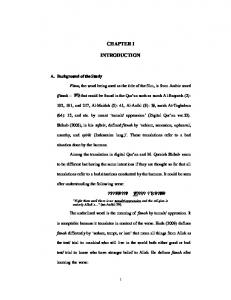
In the previous part of this chapter, the theoretical model of this study was discussed. As a result of maximizing family utility, in general, the quality of children will be determined by income, the marginal cost of having an additional child, the marginal cost of raising the child quality, and the prices of other commodities. The next discussion is an explanation of the research model used for this study. Figure 1 helps to visualize the research model of this study. As seen in Figure 1, this study focused on family efforts to invest in human capital, particularly in children. This study used two proxy determinants of investment in children, which are per capita expenditure spent for food, education, and health care and mother’s time devoted to feeding and playing with children. The study postulated that parental time investment may influence parental monetary investment. A mother has to make a time allocation decision whether she works at home to take care of her children or works in
31
I N T E R N A L
HUMAN CAPITAL INVESTMENT
F A C T O R S
PARENTAL MONETARY INVESTMENT
PARENTAL TIME INVESTMENT
OUTCOME THE QUALITY OF CHILDREN NONPHYSICAL
PHYSICAL
Figure 1. Investment in Children: Empirical Framework
32
E X T E R N A L F A C T O R S
the labor market. Whichever decision she makes, it directly and indirectly affects the investment in children. When a mother decides to spend more time working outside the home, she may sacrifice her time working at home, including her time devoted to children. In return for this sacrifice, family income may be higher, thereby the family may afford to invest more income for children. In other words, mothers’ time used both in providing child care and in generating family income may lead to higher child quality (Chiswick, 1988). When children are “time intensive,” that is when children are in the preschool and schooling years, parents need to commit a greater time investment to child care. During later years when children are more “goods intensive,” spending greater time on marketplace work would appear to be good for investment in children. A mother’s decision, whether she spends more time working in the labor market or at home, may depend on her perception of the marginal products of working in the labor market and at home (Gronau, 1974). If market wages are perceived to be lower than the compensation of nonmarket productivity, a mother tends to work at home since it is more productive. Conversely, if market wages are higher than the compensation of nonmarket productivity, she may be encouraged to participate in the labor market. Family investment in children also will be influenced by internal factors in the family, such as education of parents, particularly the mother (e.g., Leibowitz, 1972; Schoggen & Schoggen, 1968), family income (e.g., Becker, 1993; Leibowitz, 1974), gender (e.g., Leibowitz, 1974; Bian, 1996; Cronk, 1993), occupation, and other factors as well as external factors, such as residency (e.g., De Tray, 1974; Leppel, 1982; Bian, 1996) and cultural norms. Leibowitz (1972) found a positive relation between the quantity of time devoted to children and parent’s education. Meanwhile, Schoggen and Schoggen (1968) found that parent’s education also had a positive relation to the quality of time. In addition, bettereducated mothers also spend more parental monetary investment (Bian, 1996). Therefore,
33
the parent’s education may influence the parental time investment in terms of quantity and quality of time devoted to children as well as the parental monetary investment. Family income also is expected to have positive influences on parental time investment and parental monetary investment. A family with higher income may spend much more of their money and time for investment in children. Leibowitz (1974) found that family income may relate to the quality and the quantity of goods inputs. In the meantime, the family with higher income often has a housekeeper who performs all household tasks. The existence of a housekeeper may allow the mother to spend less time on household work, particularly on house cleaning, doing laundry, and cooking, and in turn, increase the mother’s time availability for investment in children. Besides the internal factors, the family investment in children may also be affected directly and indirectly by external factors, such as residency and cultural norms. De Tray (1974) found little difference in taste for child quality between rural and urban residents. Urban residents may expect much higher education for their children, as compared to rural residents. In other words, urban residence may have a positive influence on the quality of children (Leppel, 1982). Dealing with different environments, physical and economical environments, might be another explanation of the relationship between residency and the quality of children.
Instead of urban-rural differences, there may be differences in
investment in children by ethnic group. The difference in ethnic groups may not only represent the difference in cultural norms, but also indicate the difference in environment. Parental investment is expected to have an influence on the quality of children. The family that invests more in their children expects to have higher quality children. Empirical studies on investment in children often deal with a problem concerning the indicator of the quality of children, because child quality is a fairly vague concept (Behrman, 1987). The study used two proxy indicators of child quality, the child’s nutritional status and the child’s IQ score. The nutritional status represents physical quality, while the IQ score represents non-physical quality of the child.
34
Summary of the Chapter
This chapter discussed the theoretical background in examining family behavior in investment in children. The theoretical model used for this study was actually developed to examine family behavior concerning fertility. Examination of the quality of children cannot be separated from the examination of the quantity of children. The quality and the quantity of children have been postulated to be substitutes to each other. The quality of children theoretically will be determined by family income, the marginal cost of having an additional child, the marginal cost of raising child quality, and the prices of other market goods and services.
The discussion of the theoretical background was followed by
discussion of the empirical (research) model.
35
Chapter IV METHODOLOGY
This chapter reviews the data and methods of data collection and describes the analysis used to achieve the objectives of the study. A general objective was to study family behavior in the allocation of their resources to improve the quality of their children in rural families in Indonesia. The specific objectives of this study were: 1. To determine the time allocation for activities that may stimulate the child growth and development which is called parental time investment. 2. To determine the income allocation for expenses that may have the effect of increasing the quality of a child which is called parental monetary investment. 3. To identify factors that influence parental time investment and parental monetary investment to enhance the quality of children. 4. To determine the relationship between parental time investment and parental monetary investments in children. 5. To determine the impact of parental time investment and parental monetary investment on the quality of children. A description of the methodology and procedures of data collection applied in The Study on the Family in Transition, Food and Nutrition Consumption, and Child Development, operational definition of variables, data analysis, and hypotheses follow.
The Data
Source of Data
This study used the database of the Study on the Family in Transition, Food and Nutrition Consumption, and Child Development, 1993-94, which was originally collected and prepared by Guhardja, Hartoyo, Megawangi, Sumarwan, and Heryatno of the
36
Department of Community Nutrition and Family Resources, Bogor Agricultural University, Indonesia. The study on the family in transition has been conducted for three years and was funded by the Indonesian Ministry of Education. Data were collected from samples which were selected from five districts of Jakarta, the district of Wonogiri (Central Java), and the district of Agam (West Sumatera). However, this study only used data from samples collected in the districts of Wonogiri and Agam which represent rural families. The locations of these two districts can be seen in Appendix A.
Sample Selection
The population of this study was rural families in Wonogiri and Agam who had at least one child aged 2-5 years. In the original study, the selection of rural areas was based on the perception (supported by data) that those areas are the sources of migrant families for Jakarta. More families from these two districts have recently migrated to Jakarta. Therefore, samples from rural areas represent families who do not migrate and continue to live in rural areas. Initially, this sample selection procedure was an approach to determine the transition of the family due to migration. The study only used database collected from rural areas. The results of this study may not be generalizable to the broader population, but rather may serve as an initial effort to study family investment in human capital in Indonesia. Rural samples were drawn from two villages of Wonogiri, and three villages of Agam. The villages were selected purposively. Selection of villages was based on the proportion of the population who migrate to Jakarta and other cities. Researchers have maintained randomness of sample selection in each village. The total sample from these two locations includes 301 families which consist of 142 from Wonogiri, and 159 from Agam. Financial constraints limited the total number of families who participated in the study.
37
Method of Data Collection
Household data were collected by conducting an interview with the household’s wife and/or other person in the household who knew about the things being questioned. The interviews were done by trained interviewers under the supervision of the researchers. Interviewers conducted the interview with the respondents at home and observed the home environment. Respondents were asked to consult with other family members to check the accuracy of the data recorded. In terms of time allocation, the interviewers asked the respondent (mother) to recall all activities a day before the interview took place. Interviews were conducted each day of the week and the distribution of days was similar for both groups. To assess the child’s nutritional status, interviewers measured the child’s height and weight. Topics included in the questionnaires are listed in Appendix B. The intelligence quotient (IQ) test was performed by the team from the University of Diponegoro, Semarang (Central Java) and from the School of Teaching and Education Science (IKIP), Padang (West Sumatera). An expert in child intellectual development was hired by the team of researchers to organize, supervise, and verify all implementation and results of IQ tests. Because of time and financial constraints, nutritional assessment and IQ test were performed to an observed child (usually the oldest child at age 2-5 years).
Description of the Variables
Description and method of assessment of selected variables used in this study follows: Income allocation for food (FOOD).
This variable refers to per capita monthly
expenditure for food consumed both at home and away from home, and was measured in rupiah and in percentage (expenditure for food divided by total expenditures) terms. Income allocation for health care (HEALTH). This variable refers to per capita monthly expenditure for health care, such as expenses for drugs, prescriptions and medical services,
38
and was measured in rupiah and in percentage (expenditure for health care divided by total expenditures) terms. Income allocation for education (EDUC). This variable refers to per capita monthly expenditure for education, such as books, uniform, and allowances, and was measured in rupiah and in percentage (expenditure for education divided by total expenditures) terms. Parental monetary investment (HUMAN). This variable refers to per capita monthly expenditure for food, health care, and education, and was measured in rupiah and in percentage terms. Mother’s time for feeding the child (TIME5). This variable refers to the amount of time spent by the mother to feed the observed child. The variable was measured by recalling her time spent for feeding the child the day before the interview took place (in hour unit). Mother’s time for playing with the child (TIME6). This variable refers to the amount of time spent by the mother to play with the observed child. The variable was measured by recalling her time spent for playing with the child the day before the interview took place (in hour unit). Mother’s time for working (TIME1). This variable refers to the amount of time spent by the mother working outside the home. The variable was measured by recalling her time spent for working outside the home the day before the interview took place (in hour unit). Parental time investment (TIME56). This variable refers to the amount of time spent by the mother to feed and play with the observed child. The variable was measured by recalling her time spent for feeding and playing with the child the day before the interview took place (in hour unit). Child’s Nutritional Status (WAM). This variable refers to the physical nutritional status of the observed child and was assessed by using an anthropometric indicator of weight by age with reference to the standard (WAM). Children were nutritionally classified as follows: 3rd degree of undernourished if WAM is less than 60; 2nd degree if WAM is between 60 and 70; 1st degree if WAM is between 70 and 80; and normal if WAM is 80 or greater.
39
Child’s Intellectual Quotient (IQS). This variable refers to the IQ score of a child at a given time and was assessed by conducting the Stanford-Binet IQ test to children (in IQ score). For further analysis, children were classified as follows: low if the IQ score is less than 90; normal if the IQ score is between 90 and 110; and high if the IQ score is higher than 110. Parent’s education level. This variable refers to formal educational attainment of the father (FEDUC) and/or mother (MEDUC) and was measured in years of schooling. Family income (EXPEND). This variable refers to per capita total monthly expenditures (in rupiah) and was assessed by recalling all family expenses and consumption for goods and services on daily, weekly, monthly, or annual basis. Family size (SIZE). This variable refers to the number of household members who live in the same house. Family type (FAMTYPE). This variable is a dummy variable which represents the type of family (FAMTYPE=1 if a nuclear family; FAMTYPE=0 if an extended family). Mother’s occupation (MOCCUP1 & MOCCUP2). These variables are dummy variables which represent the occupation of the mother (MOCCUP1=1 if the mother worked at non-agricultural job, MOCCUP1=0 if the mother worked at other sectors or was unemployed; MOCCUP2=1 if the mother worked at agricultural job, MOCCUP2=0 if the mother worked at other sectors or was unemployed). Child’s age (AGE). The variable refers to the age of an observed child (in month). Number of school-age children (SAGE). The variable refers to the number of children who at the time of the interview attended school. Ethnic group (ETHNIC). The variable is a dummy variable representing the ethnic group (ETHNIC=1 for the Javanese families; ETHNIC=0 for the Minangese families). Child’s gender (GENDER). The variable is a dummy variable representing the gender of the observed child (GENDER=1 for boys; GENDER=0 for girls).
40
Data Analysis
The procedure for data analysis can be divided into two phases, pre-analysis and analysis. During the pre-analysis phase, such activities as coding, manual calculating, and data entry and cleaning were performed. Data coding, manual calculating, and data entry were performed by the individuals who conducted the interviews. The study used the Dbase IV software program for data entry. In the analysis phase, the researcher performed statistical analysis by using the SPSS computer package version 7.5. Procedures for statistical analysis are as follows: 1. Means and standard deviations were computed for each expenditure allocation for food, health care, and education for each ethnic group (Javanese vs. Minangese). Mean difference tests (t-tests) were performed to determine any significant difference in expenditure allocation between these two ethnic groups. 2. Means and standard deviations were computed for time allocation for child care for each ethnic group. Mean difference tests (t-tests) were performed to determine any significant difference in time allocation between these two ethnic groups. 3. Regression and correlation analyses were performed to answer the rest of the research questions. The dependent variables were parental time investment, parental monetary investment, child’s nutritional status, and child’s IQ score. The independent variables were father’s and mother’s education, family income, mother’s occupation, ethnic group, family size, family type, number of school-age children, and the child’s gender and age.
Regression models to estimate the relationship between each dependent
variable and the independent variables were presented in the following section. The ordinary-least-square method was employed to estimate regression models in this study.
41
Hypotheses
Hypothesis 1: There are no statistically significant relationships between parental time investment and internal factors (family income, mother’s time for working, mother’s and father’s education, mother’s occupation, family size, family type, and child’s age), and the external factor (ethnic group). The regression model was:
TIME56 = a1 + b1 EXPEND + b2 TIME1 + b3 MEDUC + b4 FEDUC + b5 MOCCUP1 + b6 MOCCUP2 + b7 SIZE + b8 FAMTYPE + b9 AGE + b10 ETHNIC
Hypothesis 2:
There are no statistically significant relationships between parental
monetary investment and parental time investment, internal factors (family income, mother’s time for working, mother’s and father’s education, mother’s occupation, family size, family type, and number of school-age children), and the external factor (ethnic group). The regression model was:
HUMAN = a1 + b1 TIME56 + b2 EXPEND + b3 TIME1 + b4 MEDUC + b5 FEDUC + b6 MOCCUP1 + b7 MOCCUP2 + b8 SIZE + b9 FAMTYPE + b10 SAGE + b11 ETHNIC
Hypothesis 3:
There are no statistically significant relationships between the child
nutritional status and parental monetary investment, parental time investment, internal factors (family income, mother’s time for working, mother’s and father’s education, mother’s occupation, family size, family type, child’s age, and gender), and the external factor (ethnic group). The regression model was:
42
WAM = a1 + b1 TIME56 + b2 HUMAN + b3 EXPEND + b4 TIME1 + b5 MEDUC + b6 FEDUC + b7 MOCCUP1 + b8 MOCCUP2 + b9 SIZE + b10 FAMTYPE + b11 AGE + b12 GENDER + b13 ETHNIC
Hypothesis 4: There are no statistically significant relationships between the child IQ score and parental monetary investment, parental time investment, internal factors (family income, mother’s time for working, mother’s and father’s education, mother’s occupation, family size, family type, child’s age, and gender), and the external factor (ethnic group). The regression model was:
IQS = a1 + b1 TIME56 + b2 HUMAN + b3 EXPEND + b4 TIME1 + b5 MEDUC + b6 FEDUC + b7 MOCCUP1 + b8 MOCCUP2 + b9 SIZE + b10 FAMTYPE + b11 AGE + b12 GENDER + b13 ETHNIC
The study estimated full and reduced regression models for each hypothesis. The full regression model is a model with all independent variables, while the reduced model is a model with some independent variables removed from the model.
Selection of
independent variables to be removed was based on backward stepwise procedure and/or professional judgment. The F test was performed to indicate the significance of the difference in terms of R-squared and error between the full and reduced models by using a formula, as follows (Pendhazur, 1982): (R2full - R2reduced)/(kfull - kreduced) F = ----------------------------------------(1 - R2full)/(N - kfull - 1) Where: F
= the value of calculated F ratio
R2full
= the R-squared of the full model
43
R2reduced = the R-squared of the reduced model kfull
= the number of independent variables included in the full model
kreduced = the number of independent variables included in the reduced model N
= the sample size
The calculated F ratio, then, was compared with the tabled F ratio with (kfull - kreduced) and (N - kfull - 1) degree of freedom.
Summary of the Chapter
This study was designed to investigate family behavior on investment in children and to estimate several factors that contribute to the family behavior in rural Indonesia. The study used an existing data base which was collected by researchers at the Department of Community Nutrition and Family Resources, Bogor Agricultural University, Indonesia. The specific procedures for data collection and data analysis were outlined in this chapter. In addition, the chapter also described operational definitions of variables and hypotheses.
44
Chapter V FINDINGS AND DISCUSSION
The general purpose of this study was to learn family behavior concerning their resource allocation to enhance the quality of their children and to investigate the factors that influence the family behavior of rural families in Indonesia on investing in children. The study used the database of the Study on the Family in Transition, Food and Nutrition Consumption, and Child Development 1993/94 conducted by a team of Researchers at the Department of Community Nutrition and Family Resources, Bogor Agricultural University, Indonesia. This chapter consists of five sections. The first section describes demographic characteristics of the families.
The discussion focuses on some of the
variables in the research model and the differences of these variables between two ethnic groups. The second section presents descriptive analysis of parental time and monetary investments. The third section discusses regression analysis to investigate the factors affecting parental investments (Hypotheses 1 & 2).
The fourth section presents
descriptive analysis of the child’s nutritional status and intellectual ability as proxy determinants of child quality. The five section discusses regression analysis to investigate the factors affecting child quality (Hypotheses 3 & 4).
Demographic Characteristics of the Families
The Age of the Husbands and Wives
Of the total sample, 16.9% of the husbands and 3.7% of the wives were in the age group higher than 40 years old (Table 1). The mean age of the husbands and the wives are 34.7 and 30.1 years, respectively. The sample of the study included young families, those with at least one child under five years old. The age characteristic of the husbands was not different between the ethnic groups, while that of the wives was. The average
45
Table 1. Distribution of Husbands and Wives Based on Age and Ethnic Groups Age Group (year) Husbands < 21 21 - 30 31 - 40 > 40
Javanese (n=142) Freq Percent
0 50 71 21
M sd Wives < 21 21 - 30 31 - 40 > 40 M sd
Minangese (n=159) Freq Percent
0.0 35.2 50.0 14.8
0 43 86 30
34.8 7.4
5 100 30 7
0.0 27.0 54.1 18.9
Total (n=301) Freq Percent
0 93 157 51
34.6 6.1
3.5 70.4 21.1 4.9
4 66 85 4
28.8 6.9
34.7 6.7
2.5 41.5 53.5 2.5 31.3 5.3
0.0 30.9 52.2 16.9
9 166 115 11
3.0 55.1 38.2 3.7 30.1 6.2
ages of the Javanese and the Minangese husbands were 34.8 (sd = 7.4) and 34.6 years (sd = 6.1), respectively. The mean difference of the husbands’ age between the two ethnic groups was not significant (t = .234, p > .05). The mean difference of the wives’ age was statistically significant (t = 3.522, p < .01). The average age of the Javanese wives (M = 28.8, sd = 6.9) was significantly lower than the average mean of the Minangese wives (M = 31.3, sd = 5.3).
46
Educational Background of the Husbands and Wives
Most of the husbands (69.4%) and wives (70.1%) had elementary school education (Table 2). The mean years of schooling for the husbands and for the wives were 6.6 and 6.7 years, respectively.
As a comparison, based on the 1991 Indonesia
Demographic and Health Survey, the median years of schooling for males and females in Indonesia were 5.9 and 4.3 years. It seems that even though the samples were drawn from rural areas, they had slightly higher education than did the population as a whole. One explanation of this fact is that the samples were younger and drawn from two areas in two provinces that are considered to have relatively better educational background.
Table 2. Distribution of Husbands and Wives Based on Year of Schooling and Ethnic Groups
Schooling (year) Husbands 9
Javanese (n=142) Freq Percent
11 114 10 7
M sd Wives 9 M sd
Minangese (n=159) Freq Percent
7.7 80.3 7.0 4.9
1 95 32 31
5.4 2.5
11 122 4 5
0.6 59.7 20.1 19.5
Total (n=301) Freq Percent
12 209 42 38
7.8 3.0
7.7 85.9 2.8 3.5
0 89 28 42
5.1 2.4
47
6.6 3.1
0.0 56.0 17.6 26.4 8.1 3.3
4.0 69.4 14.0 12.6
11 211 32 47
3.7 70.1 10.6 15.6 6.7 3.3
The level of education attained by both the husbands and wives was different in the two ethnic groups. The Javanese had much less education than did the Minangese for both the husbands and the wives. As seen in Table 2, only 11.9% of the husbands and 6.3% of the wives of the Javanese attended middle school or better (7 years and higher of schooling). Meanwhile, the husbands and the wives of the Minangese who had attained more than 7 years of schooling were 39.6% and 44.0%, respectively. The result of the mean difference test for years of schooling for the husbands in the two ethnic groups was statistically significant (t = 7.293, p < .01). The Javanese husbands had lower mean years of schooling (M = 5.4 years, sd = 2.5) than the Minangese husbands (M = 7.8 years, sd = 3.0). The mean years of schooling of the Javanese wives was also statistically different from that of the Minangese wives (t = 9.123, p < .01). The mean years of schooling of the Javanese wives was 5.1 years (sd = 2.4), lower than that of the Minangese wives (M = 8.1, sd = 3.4). The Javanese husbands had slightly higher education attainment than did the Javanese wives. On the contrary, the Minangese husbands had slightly less education attainment than did the Minangese wives. The fact that the Minangese wives had higher schooling may be a consequence of the traditional Minangese matriarchal system. In this system, women tend to dominate the house and to control the use of resources. They may have a greater chance to empower themselves, including gaining higher education.
The Occupations of the Husbands and Wives
Most of the husbands (65.1%) and the wives (60.1%) were involved in the agricultural sector (Table 3). These figures seem to be consistent with the general picture of the rural population in Indonesia. According to the Central Bureau of Statistics (1996), about 64.9% of the rural population 10 years of age and over worked in the agricultural sector. As reported in Table 3, there was only one sample in which the husband was unemployed while 12.6% of the wives considered themselves not employed.
48
For the Javanese, most (> 90%) worked in the agricultural sector. Those who worked in the non-agricultural sector were only 7% of the husbands and 3.5% of the wives. The Javanese husbands who did not work in the agricultural sector were working as: an industrial worker (.7%), local government officials (3.5%), and wholesalers/traders (2.8%). Meanwhile, 3.5% of the Javanese wives engage in the non-agricultural sector in areas such as: government officials (2.1%) and wholesalers/traders (1.4%). No Javanese husbands or wives reported having a second job.
Table 3. Distribution of Husbands and Wives Based on Occupation and Ethnic Groups Occupation
Husbands Not employed Agricultural Workers Non-agricultural Workers Wives Not Employed Agricultural Workers Non-agricultural Workers
Javanese (n=142) Freq Percent
Minangese (n=159) Freq Percent
Total (n=301) Freq Percent
0 132
0.0 93.0
1 64
0.6 40.2
1 196
0.3 65.1
10
7.0
94
59.2
104
34.6
3 134
2.1 94.4
35 47
22.0 29.5
38 181
12.6 60.1
5
3.5
77
48.4
82
27.2
The Minangese, in the other hand, had much more variety of occupation. As seen in Table 3, only 40.2% of the Minangese husbands and 29.5% of the wives worked in the agricultural sector. The husbands who did not work in the agricultural sector were working as: wholesalers/ traders (27.5%), self-employed in clothing and other services
49
(20.1%), government services (7.5%), and industrial workers (4.4%). About 29.6% of the Minangese husbands reported having a second job. The Minangese wives (48.4%) who reported themselves as having non-agricultural jobs were working as: wholesalers/traders (29.6%), government officials (10.7%), self-employed (7.5%), and industrial workers (.6%). About 20.8% of the Minangese wives had a second job. The Javanese families seemed to rely mainly on agricultural activities. According to Koentjaraningrat (1985), about 82.5% of the Javanese still lived as peasants in village communities, agrarian matters, and subsistence agriculture forms. Meanwhile the Minangese families depended less on agricultural activities. The differences in the cultural background, the education level, and the job opportunities may contribute to the difference in occupation of Javanese and Minangese husbands and the wives.
Family Size and Number of Children
As seen in Table 4, about 78.0% of the families had three children or less. The mean number of children was 2.5 (sd = 1.6). Results of the 1991 Indonesia Demographic and Health Survey indicated that the mean number of children ever born to women ages 40-49 was about 4.90.
Because the couples in this study were still in the reproductive
phase, it is understandable that the mean number of children was lower than the mean number of children ever born for Indonesia women. The Javanese families seemed to have fewer children than the Minangese families. As reported in Table 4, more of the Javanese families (93.7%) than the Minangese families (64.1%) had three children or less. There was a statistically significant difference in the mean number of children of the Javanese and the Minangese (t = 6.713, p < .01). The mean number of children of the Javanese families was 1.9 (sd = 1.1), lower than that of the Minangese families (M = 3.0, sd = 1.7). As seen in Table 4, most of the families (44.9%) had four to five members. The mean number of family members was 5.5 (range from 3 to 12, sd = 1.6). The Minangese
50
had larger families than the Javanese. About 59.1% of the Minangese families had six family members or higher, compared to only 30.3% of the Javanese families.
The
difference in the mean number of family members between the Javanese and the Minangese families was also statistically significant (t = 5.384, p < .01). The mean number of family members of the Javanese families was 5.0 (sd = 1.4), meanwhile that of the Minangese families was 5.9 (sd = 1.6). Table 4. Distribution of Families Based on Family Size, Number of Children and Ethnic Groups
Javanese (n=142) Freq Percent Number of Children (person) 5
62 71 6 3
M sd
43.7 50.0 4.2 2.1
35 67 43 14
1.9 1.1
M sd Family Size (person) 7
Minangese (n=159) Freq Percent
19 80 36 7
22.0 42.1 27.0 8.8
Total (n=301) Freq Percent
97 138 49 17
3.0 1.7
13.4 56.3 25.4 4.9
10 55 67 27
5.0 1.4
51
2.5 1.6
6.3 34.6 42.1 17.0 5.9 1.6
32.2 45.8 16.3 5.6
29 135 103 34
9.6 44.9 34.2 11.3 5.5 1.6
Summary of the Section
The families who participated in this study were typically young, less-educated families with three children or less. As typical rural families, most of them were involved in the agricultural sector. The characteristics of the Javanese families were different from those of the Minangese families.
The Javanese families had lower educational
background, fewer children and family members, and relied mainly on the agricultural sector. Minangese families had higher educational background, more children and family members, and much more variety in occupation.
Parental Time and Monetary Investments
The focus of this section is to describe parental monetary and time investments in children and to investigate the factors that influence family behavior on investing in children. Parental monetary investment is all family income spent for expenses that may result in increasing the quality of children. The expenses which are considered to be the parental monetary investment are education, health care, and food.
Parental time
investment is all the time parents, particularly the mothers, spend with their children.
Parental Time Investment
This study focused on time spent by the mothers as an indicator of parental time investment. As mentioned in the previous chapter, the mother is the main care taker of the children in the family.
Bryant and Zick (1996) distinguished two types of parental time
investment, which are: primary and secondary parental time investment. Primary child care time is basically all the time parents spend with their children without parents doing something else.
Examples of primary time would be the time spent playing, eating, and
working with children. While secondary parental time is the time spent with children when
52
primarily doing something else, for example taking care of children while primarily cooking or helping a child with homework while primarily cleaning a bedroom. Bryant and Zick noted that secondary child care time needed to be explored more. In the study, mothers’ time can be categorized into such activities as: working outside the home, leaving the home with the child, performing household work, doing household work while the child is along, feeding the child, playing with the child, sleeping with the child also sleeping, sleeping alone, and conducting other activities. Mothers’ activities which are considered as “leaving home with the child” usually consist of visiting neighbors, shopping, and attending social gatherings. During these activities, the mother usually takes the observed child with her. Meanwhile, conducting other activities includes performing personal care and prayer. All these activities can be grouped into: the primary time investment (i.e., time spent feeding the child and playing with the child), the secondary time investment (i.e., time spent doing housework while the child is with the mother), and time non-investment (i.e., time spent working, sleeping with and/or without the child, doing household work, and conducting other activities). The mothers’ time allocation of the Javanese and the Minangese is presented in Table 5. The pattern of time allocation of the mothers differs between the Javanese and the Minangese. The Javanese mothers spent significantly more time working outside the home, playing with the child, and sleeping alone.
The Minangese mothers spent
significantly more time doing household work, feeding the child, sleeping with the child, and performing other activities. Total mother’s time spent with the child while she did something else (the secondary time investment) was not significantly different between the Javanese and the Minangese mothers. The Javanese mothers spent an average of 3.33 hours (sd = 3.05) working outside the home, compared to 1.91 hours (sd = 2.26) for the Minangese mothers (Table 5). One explanation of this finding may be attributed to the fact that more than one-fifth of the Minangese mothers, as compared to only 2.1% of the Javanese mothers, were not working. In addition, most of the mothers seemed to work part time. Since they worked
53
on their farm land, they also had relatively flexible work schedules. These factors made the average hours working outside the home low, particularly for the Minangese mothers. Because the greater percentage were not working, on the average, the Minangese mothers spent one-hour longer in household work than did the Javanese mothers. The Minangese mothers spent about 4.64 hours (sd = 2.67), while the Javanese mothers spent about 3.55 hours (sd = 2.06) for household work, such as cooking, doing laundry, and cleaning.
The number of children and family members may be another factor that
influences the time spent on household work. The time spent for household work is positively influenced by the size of the family (Nickols & Metzen, 1978; Walker & Woods, 1976).
As mentioned in the previous section, the Minangese families had a greater
number of children and family members than the Javanese families.
Table 5. Daily Time Allocation of the Mothers (in hour units)
Activity
Work outside the home Outside the home w/ the child Household work Household work w/ the child Feed the child Play w/ the child Sleep accompanied by the child Sleep without the child Other Total
Javanese (n = 142) M sd
Minangese (n = 159) M sd
3.33 1.05 3.55 3.46 0.73 2.49 5.33 2.96 1.10
1.91*** 1.14 4.64*** 3.50 1.30*** 1.07*** 6.94*** 1.72*** 1.78***
3.05 2.03 2.06 2.66 0.86 2.02 3.92 3.81 1.97
24.00
24.00
***
Significantly different at the .01 level
54
2.26 1.88 2.67 2.52 0.94 1.26 2.83 2.86 2.46
The Minangese mothers spent about one-half hour longer feeding the child than did the Javanese mothers (t = 5.468, p < .05). Meanwhile, the Minangese mothers spent significantly less time playing with the child (about one and a half hour less) than did the Javanese mothers (t = 7.253, p < .05). Time spent for both feeding the child and playing with the child, according to Bryant and Zick (1996), are considered to be primary child care time in which the mothers devote their time only to the child without doing something else. The study considers these two activities as the primary time investment, since during these times the interaction between the mother and the child may stimulate better child growth and development. The time spent sleeping with and without the child is also significantly different between the Javanese mothers and the Minangese mothers. An under five-year-old child usually sleeps in the same bed as the mother does during the night. The mother may have an opportunity to sleep without the child during the day when other family members take care of the child. The average time for sleeping with the child for the Minangese mothers (M = 6.94 hours, sd = 2.83) was significantly longer than the Javanese mothers (M = 5.33 hours, sd = 3.92). The Javanese mothers, however, spent longer time for sleeping without the child during the day (M = 2.96 hours, sd = 3.81) than did the Minangese mothers (M = 1.72 hours, sd = 2.86). The study defined time spent for “other” as all the time devoted for activities which were not previously mentioned, such as personal care and praying. For these activities, the Minangese mothers spent about 1.79 hours (sd = 2.46), significantly longer time than did the Javanese mothers (M = 1.10 hours, sd = 1.97). Minangese are considered to be more religious and spend more time for religious activities, including praying. This might be one possible explanation of the fact that the Minangese mothers spent significantly longer time on this category than the Javanese mothers.
55
Parental Monetary Investment in Children
As seen in Table 6, per family monthly monetary expenditure of the Javanese was significantly different from that of the Minangese (t = 8.710, p < .01). The Javanese families spent on average Rp 120,050 (sd = 57,900), about 40% less than spent by the Minangese families (M = Rp 202,190, sd = 101,300). Per capita monthly expenditure of the Javanese was also significantly lower than the Minangese (t = 5,732, p < .01). The Javanese spent Rp 25,190 (sd = 12,700) per capita monthly, about 28% less than spent by the Minangese (M = Rp 35,100, sd = 17,000). The difference between the Javanese and the Minangese was smaller in per capita monthly expenditure than in per family monthly expenditure.
Table 6. Average Monthly Family and Per Capita Expenditure (in thousand rupiah)
Expenditure Items Family Food Non-Food Education Health Others Total Per Capita Food Non-Food Education Health Others Total
Javanese (n = 142) M sd
Minangese (n = 159) M sd
73.20
35.10
127.00***
55.96
2.05 1.97 42.83 120.05
7.02 3.16 26.91 57.90
5.43 2.64 67.11*** 202.19***
22.65 3.35 45.39 101.28
15.38
7.85
22.15***
10.27
0.38 0.40 9.04 25.19
1.35 0.61 6.13 12.70
0.70 0.48 11.72*** 35.06***
2.45 0.78 7.78 16.96
Note: ***Significantly different at the .01 level. US$1 = Rp 2,169 (1994)
56
As a comparison, average per capita monthly expenditure for the rural population of Indonesia in 1993 was Rp 33,385 (Central Bureau of Statistics, 1995). The rural population in Central Java seems to have a lower income than those in West Sumatera. Data from the Central Bureau of Statistics (1995) indicated that the estimated median monthly expenditure of the rural population in the Central Java Province was Rp 24,260, while in the West Sumatera Province it was Rp 37,810 (calculated from Table 10.2.10, p. 556-557).
Those in the study seem to represent the general situation of the rural
population in the two areas of the study. The Javanese spent Rp 15,380 per capita on food or about 61.0% of the total expenditure. Meanwhile, the Minangese families spent Rp 22,150 per capita on food or about 63.2% of the total.
As a comparison, on the average, the rural population in
Indonesia spent about 63.6% of the total expenditure on food (Central Bureau of Statistics, 1995). Even though the difference in per capita food expenditure in rupiah was statistically significant between the Javanese and the Minangese (t = 6.446, p < .01), the difference in the percentage of the food expenditure was insignificant (t = 1.756, p > .05). The amount of expenditure for both education and health care was not statistically significant between the Javanese and the Minangese. The Minangese spent a slightly higher amount for education and health care than did the Javanese. For education, the Minangese spent monthly about Rp 700 per capita, almost twice as much as spent by the Javanese (Rp 380). In terms of percentage, the Minangese spent about 2.0% of the total on education, compared to 1.5% spent by the Javanese. Most families in the sample were young families in which the children were still in the elementary school. In fact, some families had no school-age children. As a consequence, on the average, they spent a small portion of their expenditure on education. Compared to the average spending for education for the Indonesian population (2.9% in 1993; Maksum, 1997), the Javanese and the Minangese families in the study spent a smaller portion of the total expenditure on education.
57
The fact that the sample
was drawn from the rural area might be a possible explanation of the phenomenon that their spending on education was smaller than the average spending of the population. In terms of rupiah, the Minangese spent about Rp 480 per capita per month for health care, higher than did the Javanese (Rp 400). However, in terms of the percentage, the Javanese spent a greater portion of the total expenditure on health care than did the Minangese. The Javanese spent 1.6%, while the Minangese spent 1.4% of the total expenditure on health care.
Typical spending on health care was to purchase non-
prescription drugs for such sicknesses as headache, cold, and fever. Compared to the national figures (1.3% in 1993; Maksum, 1997), the families in this study spent a slightly higher portion of the total expenditure on health care. The amount of expenditure for other commodities/services were Rp 9,040 for the Javanese and Rp 11,720 for the Minangese. The difference between two means was statistically significant (t = 3.330, p < .01). However, in terms of the percentage, per capita monthly expenditure for other commodities of the Javanese was not significantly different from that of the Minangese. Both the Javanese and the Minangese spent about one-third of the total expenditure for other commodities and services, such as housing, utilities, transportation, recreation, taxes, and donations. The differences in expenditure allocation between the Javanese and the Minangese were statistically significant in nominal (Rupiah) terms, but not significant in relative (percentage) terms. This indicates that even though the Javanese and the Minangese had different levels of income (total expenditure), these two ethnic groups had similar expenditure patterns.
Factors Affecting Parental Time Investment
In general, feeding practices may affect child development and health (Auld & Morris, 1994). While the mother feeds the child, she often teaches the child some other things, including manners and values. Play, on the other hand, is life for young children
58
and relates to child development and learning (Rogers & Sawyers, 1995). Gottfried (1985) stated that the two most potent and pervasive influences on the child’s cognitive development are the parent involvement, particularly the mother, and the provision of play materials. These are reasons why the study paid attention to the time spent by the mother for feeding the child and for playing with the child as indicators of parental time investment. Summaries of regression analysis for the variables predicting parental time investment are presented in Tables 7, 8, and 9. The dependent variables of the parental time are the amount of time spent by the mother for feeding the child (TIME5), for playing with the child (TIME6), and for both feeding and playing with the child (TIME56).
Meanwhile, the independent variables are total family expenditure
(EXPEND), the amount of time spent by the mother for working outside the home (TIME1), the mother’s education (MEDUC), the father’s education (FEDUC), dummy variables of the mother’s occupation (MOCCUP1 & MOCCUP2), family size (SIZE), dummy variable of the type of family (FAMTYPE), the age of the observed child (AGE), and dummy variable of the ethnic groups (ETHNIC). For each dependent variable, the study estimates two regression models, those are: full and reduced models. The full model is a model with all independent variables, while the reduced model is a model with some independent variables dropped from the model. There were no statistically significant differences between any full model and its corresponding reduced model in terms of Rsquared and error.
Mother’s Time Feeding the Child
Table 7 presents the summary of regression analysis for the variables predicting time spent for feeding the child (TIME5) using Ordinary Least Square (OLS). As seen in the Table 7, the R-squared of the full model was .183 and it is statistically significant at the .01 level. It means that the all independent variables account for about 18.3% of the
59
Table 7. Summary of Regression Analysis for Variables Predicting Time Spent Feeding the Child (N = 262)
Model Variable
Full β
B Intercept Family Expenditure (EXPEND) Mother’s Work Time (TIME1) Mother’s Education (MEDUC) Father’s Education (FEDUC) Non-agricultural Job or Unemployed (MOCCUP1) Agricultural Job or Unemployed (MOCCUP2) Family Size (SIZE) Type of family (FAMTYPE) Child’s Age (AGE) Ethnic group (ETHNIC)
2.113 (.446) .001 (.001) -.062 (.022) .027 (.026) -.004 (.025) .070 (.189) .147 (.200) -.051 (.045) .033 (.122) -.023 (.005) -.319 (.162)
R-squared F ratio
Reduced
.183 5.62***
.122* -.169***
β
B 2.459 (.306) .002 (.001) -.059 (.022)
.144** -.160***
.091 -.013 .033 .076 -.082
-.067 (.040)
-.107*
-.023 (.005) -.330 (.125)
-.267***
.017 -.256*** -.166**
-.172***
.178 11.05***
Note. Standard error is in parentheses; * significant at the .10 level; ** significant at the .05 level; and
***
significant at the .01 level; B is unstandardized regression coefficient; β is
standardized regression coefficient.
60
variance in TIME5.
The R-squared of the reduced model was .178 and it is also
statistically significant at the .01 level. The change in the R-squared was very small (about .5%) and not significant (Appendix C), even though five variables were removed from the model. This means that the reduced model was as good as the full model in explaining the relationship between independent variables and dependent variable of the time spent feeding the child. Neither the mother’s nor the father’s education significantly affects the time spent by the mother feeding the child. The length of time the mother feeds the child also was not significantly influenced by the mother’s occupation (whether she worked outside the home in the farm, in industry, or not at all) as well as by the family type (whether nuclear or extended family). In the full model, the impact of the family size on the time feeding the child was also insignificant. However in the reduced model, the impact of the family size on the time for feeding the child became statistically significant. Whether the family is extended or nuclear has no impact on the amount of time spent by mother feeding the child. This study found that most Javanese extended families usually consist of the nuclear family and grandmother/grandfather, while Minangese extended families consist of the nuclear family, grandmother/grandfather, and other relatives (aunts/uncles and nieces/nephews) from the mother’s line. The presence of other adult members in the family did not change the amount of time spent by the mother in feeding the child. This means that the mother is the major person who performs the task to feed the child. The number of family members, however, has a negative and significant relationship with the time spent by the mother for feeding the child. The mother of the large family may spend less time for feeding the observed child than the mother of the small family. This might not be because some other family members took over the job to feed the child, but rather because the mother had to spend more time for housework due to large family size. The amount of time spent for household work has a positive correlation with the number of family members (Walker & Woods, 1976). As a result of
61
this situation, the mother has less time available for other activities, including for feeding the child. The age of the observed child (AGE) also had a negative and statistically significant impact on the time for feeding. Controlling other variables, the mother with an older observed child may spend less time compared to the mother with a younger child. An older child seems to develop more feeding skills than the younger ones. As the age of the child increases, the child develops self-feeding skills (Pipes & Trahms, 1996) requiring the mother to spend less time. The total family expenditure as an approach to determine the family income had a positive and significant relationship with the time spent feeding the child. In a richer family, the mother spent more time to feed the child than in a poorer family, holding other variables constant. A richer family in rural areas tends to have a household helper to perform dirty and hard household work, such as cleaning the house and backyard, doing laundry and ironing, and cooking. Therefore, the mother in a richer family may have more time available to do light household work, including feeding the child. Since feeding the child is perceived to impact the health and nutritional status of the child, the mother usually does not want a substitute to perform this task. Ethnic group and the time spent working outside the home had negative and significant relationships with the time spent feeding the child. The Javanese mother spent less time to feed the child as compared to the Minangese mother. In the meantime, the mother who spent more time working outside the home devoted less time to feeding the child. The availability of the mother’s time seems to explain this relationship. As the mother spends more time working outside the home or doing other housework, she may have less time available for feeding the child. Looking at the absolute value of the standardized regression coefficients, the impact of the age on the time spent feeding the child was the highest. The standardized regression coefficient for the child’s age was -.267. It means that with an increase of one standard deviation of the child’s age, the amount of time spent feeding the child may
62
decline by .267 standard deviation. This indicates that the age of the child, particularly the youngest ones, is the most important variable in determining the time allocation, in general.
Mother’s Time Playing with the Child
Table 8 presents a summary of the regression analysis for variables predicting time spent playing with the child (TIME6). As seen in Table 8, the R-squared for the full model was .252 and it was statistically significant at the .01 level. About 25.2% of the variation of the TIME6 was explained by the variation of independent variables in the model. In the full model, the amount of time spent by the mother playing with the child was significantly influenced by time spent working (TIME1), the type of family (FAMTYPE), and the ethnic groups (ETHNIC). By taking out six variables, the Rsquared changed to .235. The change of the R-squared was insignificant (Appendix C). It means that the reduced model was as good as the full model in estimating the relationship between independent variables and the dependent variable of the time spent for playing with the child.
In the reduced model, the variables which have a significant
effect on the time spent for playing with the child were the amount of time for working (TIME1), the type of family (FAMTYPE), the ethnic group (ETHNIC) and the mother’s education. Ethnic group seems to have the greatest impact on the time spent playing with the child. The Javanese mother spent more time playing with the child than did the Minangese mother. Time spent by the mother working outside the home has also a negative and significant relationship with the time spent playing with children. The availability of the mother’s time seems to be the explanation to this fact. Therefore, the mother who spent more time working in the labor market, because of less time available, spent less time playing with the child.
This might have a negative impact on the child’s cognitive
development since the mother is less involved in playing with her child.
63
Table 8. Summary of Regression Analysis for Variables Predicting Time Spent Playing with the Child (N = 262)
Model Variable
Full β
B Intercept Family Expenditure (EXPEND) Mother’s Work Time (TIME1) Mother’s Education (MEDUC) Father’s Education (FEDUC) Non-agricultural Job or unemployed (MOCCUP1) Agricultural Job or unemployed (MOCCUP2) Family Size (SIZE) Type of family (FAMTYPE) Child’s Age (AGE) Ethnic group (ETHNIC)
2.445 (.817) .002 (.001) -.165 (.041) .035 (.048) .009 (.046) -.311 (.346) .450 (.367) -.124 (.082) -.563 (.223) -.015 (.009) 1.247 (.296)
R-squared F ratio
Reduced
.252 8.44***
β
B 1.011 (.388)
.077 -.234*** .062
-.183 (.040) .065 (.037)
-.259***
-.451 (.205)
-.123**
1.378 (.275)
.375***
.114*
.015 -.077 .121 -.104 -.154** -.089 .340***
.235 15.74***
Note. Standard error is in parentheses; * significant at the .10 level; ** significant at the .05 level; and
***
significant at the .01 level; B is unstandardized regression coefficient; β is
standardized regression coefficient.
64
The standardized coefficient for FAMTYPE was -.123 and it is significant at the .01 level. The study set FAMTYPE = 0 for the extended family and FAMTYPE = 1 for the nuclear family. It means that the mother in a nuclear family may spend less time in playing with the child than the mother in a extended family. The presence of other adult family, members, such as a grandparent, uncle, aunt, and other relatives may have benefit in helping the mother take care of housework. As a consequence, the mother in the extended family may have more time to play with the child as compared to the mother in a nuclear family. Time devoted to playing with the child was positively and significantly influenced by the mother’s education. The mother with higher education may devote more time to play with the child. This finding indicates that the mother with higher education does not always go to work and spend more time in the labor market. In addition, she may have more concern about child development and commit herself to be more involved in child care. Research done in the US indicated that parent education and income play a strong role in determining appropriate child care for children (Leibowitz, Waite, & Witsberger, 1988). Education tends to make the parent exposed to knowledge of the benefits of nursery school and other knowledge about child development, and in turn, the parent becomes more aware and concerned about child growth and development. In this study, putting the child in a nursery school or play group is out of the question because this child care service is not available in rural areas in Indonesia. The mother with higher education may increase her concern about child development. As a consequence, she may devote more time and effort to child development, including spending more time playing with the child.
65
Parental Time Investment
Table 9 presents a summary of regression analysis for variables predicting total time spent for feeding and playing with the child (TIME56). The variable of TIME56 was considered to be the total parental time investment in this study. The R-squared of the full model was .231 and it is significantly different from zero at the .01 level. By removing three variables of MEDUC, FEDUC, and MOCCUP1, the R-squared decreased by only .008. The change in the R-squared was not significant (Appendix C). The reduced model was as good as the full model. The independent variables in the model contribute slightly less than one-fourth of the variance of the total parental time investment. The results of estimation of the full model were similar to the two previous models. As seen in Table 9, the total parental time investment was significantly and positively influenced by the total expenditure (EXPEND) and the ethnic group (ETHNIC), and negatively by
TIME1, FAMTYPE, and AGE. In the reduced model, the
impact of MOCCUP2 (whether the mother works in agriculture or is unemployed) and the family size on the time spent feeding and playing appeared. The impact of the family size (SIZE) on the time spent feeding and playing was consistent with previous findings as well as the impacts of such independent variables as the total expenditure (EXPEND), the time spent by the mother for working (TIME1), the family type (FAMTYPE), the age of the child (AGE), and the ethnic group (ETHNIC). In addition to these variables, the total parental time investment was also significantly and positively influenced by whether the mother worked in agriculture or was unemployed (MOCCUP2). The mother who worked in an agricultural job spent more time on the total parental time investment as compared to those who were unemployed.
Those who
worked in a non-agricultural job, however, had an insignificantly different investment in time for children than those who were unemployed. The mothers who worked in an
66
Table 9. Summary of Regression Analysis for Variables Predicting Total Time Spent Feeding and Playing with the Child (N = 262)
Model Variable
Full β
B Intercept Family Expenditure (EXPEND) Mother’s Work Time (TIME1) Mother’s Education (MEDUC) Father’s Education (FEDUC) Non-agricultural Job or Unemployed (MOCCUP1) Agricultural Job or Unemployed (MOCCUP2) Family Size (SIZE) Type of family (FAMTYPE) Child’s Age (AGE) Ethnic group (ETHNIC)
4.568 (.938) .003 (.002) -.227 (.047) .062 (.055) .005 (.053) -.241 (.397) .597 (.421) -.176 (.094) -.529 (.256) -.038 (.011) .928 (.340)
R-squared F ratio
Reduced
.231 7.52***
.124* -.284***
β
B 5.120 (.709) .003 (.002) -.226 (.047)
.145** -.283***
.097 .007 -.053 .142 -.130 -.128** -.197*** .223***
.630 (.319) -.202 (.089) -.574 (.250) -.039 (.011) .826 (.330)
.150** -.150** -.139** -.205*** .199**
.223 10.43***
Note. Standard error is in parentheses; * significant at the .10 level; ** significant at the .05 level; and
***
significant at the .01 level; B is unstandardized regression coefficient; β is
standardized regression coefficient.
67
agricultural job spent an average of 3.03 hours (sd = 2.09) on parental time investment, compared to 2.37 hours (sd = 1.62) for those who worked in the non-agricultural sector and 2.34 hours (sd = 2.24) for unemployed mothers. These findings are difficult to explain. In terms of time available for household work and enhancing child quality, unemployed mothers would have greater time than working mothers, in general. Because of time availability, unemployed mothers are postulated to devote more time for investment in children than working mothers. However, the study found the relationship to be opposite, a working mother, particularly one who worked in agriculture, had a greater parental time investment than the unemployed mother. Time availability may not be the only explanation concerning decision about parental time investment. Based on the findings, the study rejected hypothesis 1 which stated “There are no statistically significant relationships between the parental time investment (mother’s time spent for feeding the child, for playing with the child, or for both activities) and internal factors (family expenditure, mother/father’s education, family size, family type, mother’s occupation, mother’s time for working, and the age of the child) and the external factor (ethnic group).” Internal and external factors taken together do affect the parental time investment significantly.
The impact of total family expenditure (EXPEND), mother’s
occupation (MOCCUP2), and ethnic group (ETHNIC) were positive and significant, while that of the time spent by the mother for working (TIME1), family size (SIZE), the age of the child (AGE), and family type (FAMTYPE) were negative and significant on the parental time investment.
Factors Affecting Parental Monetary Investment
The parental monetary investment refers to the parents’ total expenditures on the child, including money spent for food, clothing, books, medical care, toys, allowances, and recreational activities (Bian, 1996). Since the variable of the parents’ total expenditures specific to the child was not available, the study used monthly per capita expenditure for
68
food, education (books and fees), and health care. These are crude indicators of the parental monetary investment because these indicators might not capture the human capital effort directly to the child.
However, the study assumed that the parents’
expenditures on the child have a positive correlation with per capita expenditure. It means that a family that spent much more per capita on food may reflect a higher child’s expense for food as compared to those who spent less. The study investigated the parental monetary investment by using four indicators: monthly per capita expenditure for food (FOOD), education (EDUC), health (HEALTH), and for food, education, and health combined (HUMAN).
These expenditures are
considered to be the parental monetary investment because of their impact on the quality of children. Meanwhile, independent variables are total family expenditure (EXPEND), mother’s time for working (TIME1), mother’s parental time investment (TIME56), mother’s education (MEDUC), father’s education (FEDUC), mother’s occupation (MOCCUP1 & MOCCUP2), family size (SIZE), family type (FAMTYPE), number of school age children (SAGE), and ethnic group (ETHNIC). Summaries of regression analysis for variables predicting parental monetary investment are presented in Tables 10, 11, 12, and 13.
Expenditure for Food
Table 10 presents a summary of the regression analysis for variables predicting per capita expenditure for food. In the full model, the R-squared was .769 and it is significant at the .01 level. It means that about 76.9% of the variation of per capita expenditure for food was explained by the variation of independent variables taken together in the model.
It is noted that four independent variables had insignificant
relationships to per capita expenditure for food. These variables were: mother’s and father’s education (MEDUC & FEDUC), mother’s time spent for working (TIME1), and whether the mother works in non-agricultural jobs or is unemployed (MOCCUP1).
69
Table 10. Summary of Regression Analysis for Variables Predicting Monthly Per Capita Expenditure for Food (N = 299)
Model Variable
Full
Reduced β
B Intercept Family Expenditure (EXPEND) Mother’s Work Time (WORK1) Parental Time Investment (TIME56) Mother’s Education (MEDUC) Father’s Education (FEDUC) Non-agricultural Job or Unemployed (MOCCUP1) Agricultural Job or Unemployed (MOCCUP2) Family Size (SIZE) Type of Family (FAMTYPE) Number of School-age Children (SAGE) Ethnic Group (ETHNIC)
21.974 (2.308) .101 (.004) .007 (.113) -.246 (.152) -.109 (.135) .051 (.130) -1.030 (.981) 2.346 (1.053) -3.049 (.306) 1.211 (.782) -1.480 (.409) -4.388 (.830)
R-squared F ratio
.964***
β
B 20.606 (1.919) .100 (.004)
.948***
.002 -.051
-.252 (.144)
-.052*
3.123 (.791) -2.973 (.300) 1.350 (.766) -1.481 (.400) -4.259 (.801)
.156***
-.036 .016 -.047 .118** -.498*** .062 -.176*** -.224***
.769 86.88***
-.486*** .069* -.176*** -.218***
.768 137.25***
Note. Standard error is in parentheses; * significant at the .10 level; ** significant at the .05 level; and
***
significant at the .01 level; B is unstandardized regression coefficient; β is
standardized regression coefficient.
70
When these three variables were removed from the model, the R-squared decreased by .001 to .768 and it is significant at the .01 level. The statistical test for the change in the R-squared resulted in an insignificant difference between the reduced and the full model (Appendix C). The reduced model was as good as the full model in explaining the variable predicting monthly per capita expenditure for food. As seen in Table 10, the total family expenditure had a dominant impact on per capita expenditure.
The relationship between these two variables was positive and
significant with a standardized coefficient of .964. It means that every one standard deviation change of total family expenditure caused a change of almost one standard deviation of per capita expenditure for food. It is a common relationship. As higher family income was reflected by total family expenditure, more money was spent for food and for everything else. A richer family can purchase more goods and services than a poorer family. In terms of percentage, total family expenditure, however, had a negative and significant relationship with per capita expenditure for food (Appendix D). It means that a richer family spends less percentage of the income on food than a poorer family. This finding was consistent with Engel’s theory and the findings from other studies. Engel observed that as total expenditure increases a family spends a smaller portion on food (Lino & Johnson, 1995). The finding indicates that income elasticity of expenditure for food is less than one (Sawtelle, 1993; Blaylock & Smallwood, 1986; Abdel-Ghany & Foster, 1982; Abdel-Ghany & Sharpe, 1997). The family size had a negative and significant impact on per capita expenditure for food. A family with a greater number of family members may spend less per capita on food as compared to those with fewer family members. The number of family members may become a constraint, particularly for a poor family, in achieving better child quality. This is one explanation to the child quantity - quality relationship. Given a level of family resources, a family with a greater number of children may have less ability to invest in
71
children. In later sections, negative and significant relationships between family size and per capita expenditure for education and health care are discussed. Whether the mother works in an agricultural job or is unemployed (MOCCUP2) also had a significant relationship to per capita expenditure for food. Holding other variables constant, on the average, a family with a mother who works in an agricultural job may have about Rp 3,123 higher per capita expenditure for food than a family with an unemployed mother.
Also, whether the mother works in non-agricultural job
(MOCCUP1) had an insignificant impact on the per capita expenditure for food. Based on these findings, the family may get more economic benefit from an agricultural employed mother than from non-agricultural employed mother. The ethnic group has a significant impact on per capita expenditure for food. The Javanese families spend less per capita for food than the Minangese families. In terms of percentage, the Javanese families also spend a smaller portion of their income on food. These findings indicate that consumer behavior of the Javanese differs from that of the Minangese. The difference in per capita expenditure for food in nominal and percentage terms between the Javanese and the Minangese was clearly not because of the difference in other variables between these two ethnic groups. Whether the family was nuclear or extended (FAMTYPE) had a significant influence on per capita expenditure for food. An extended family had a lower per capita expenditure for food as compared to a nuclear family, holding other variables constant. This seems consistent with the impact of family size. Both variables were in the model and had significant impact on per capita expenditure for food. Therefore, the impact of the type of family was significant on per capita expenditure on food even when all other variables, including the family size stayed the same. The number of school-age children had a significant and positive influence on per capita expenditure for food. A family with greater number of school-age children spends less per capita for food. School-age children required greater expenses particularly on education. The study found that the number of school-age children had a positive and
72
significant relationship with per capita expenditure for education in nominal and percentage terms (discussed in a later section). Parental time investment, indicated by the mother’s time spent for feeding and playing with the child (TIME56), had a negative and significant relationship with per capita expenditure for food. A family whose mother spent more time for feeding the child and playing with the child may devote less per capita for food. This finding indicated that, holding other variables constant, an increase of one hour of time spent by the mother for investment in children may decrease per capita expenditure for food by about Rp 252 per month.
Expenditure for Education
Table 11 presents a summary of the regression analysis for variables predicting per capita expenditure for education. In the full model, the independent variables, family expenditure (EXPEND), family size (SIZE), number of school-age children (SAGE), and ethnic group (ETHNIC), had significant relationships with per capita expenditure for education. The R-squared for the full model was .287 and it is significant at the .01 level. After removing six independent variables from the model, the R-squared was .278. The change in R-squares between the two models was not significant (Appendix C). The reduced model was as good as the full model in explaining the relationship between dependent and independent variables. As seen in Table 11, total family expenditure had a positive and significant relationship with per capita expenditure for education.
The impact of total family
expenditure was less on per capita expenditure for education than on per capita expenditure for food. Family expenditure had a standardized coefficient of .340 on per capita expenditure for education as compared to .948 on per capita expenditure for food. However, in terms of elasticity, the per capita expenditure for education was more income elastic than per capita expenditure for food. Calculated income elasticity for education
73
Table 11. Summary of Regression Analysis for Variables Predicting Monthly Per Capita Expenditure for Education (N = 299)
Model Variable
Full β
B Intercept Family Expenditure (EXPEND) Mother’s Work Time (WORK1) Parental Time Investment (TIME56) Mother’s Education (MEDUC) Father’s Education (FEDUC) Non-agricultural Job or Unemployed (MOCCUP1) Agricultural Job or Unemployed (MOCCUP2) Family Size (SIZE) Type of Family (FAMTYPE) Number of School-age Children (SAGE) Ethnic Group (ETHNIC)
.222 (.831) .008 (.001) -.047 (.041) -.058 (.055) -.039 (.049) -.056 (.047) .012 (.353) -.211 (.379) -.217 (.110) -.379 (.281) .793 (.147) .780 (.299)
R-squared F ratio
Reduced
.287 10.52***
.355***
β
B -.496 (.656) .007 (.001)
.340***
-.065 -.058 -.064 -.009 .003 -.052 -.173** -.095 .460*** .195***
-.199 (.107) -.308 (.274) .796 (.142) .648 (.230)
-.159* -.077 .461*** .162***
.278 22.52***
Note. Standard error is in parentheses; * significant at the .10 level; ** significant at the .05 level; and
***
significant at the .01 level; B is unstandardized regression coefficient; β is
standardized regression coefficient.
74
was 2.08, compared to .85 for food and 1.09 for health care.1 It means that for every one percent increase of total family expenditure, per capita expenditure increases by 2.08%, .85%, and 1.09% for education, food, and health care, respectively. The facts that income elasticities for education and health care tend to be more elastic are consistent with AbdelGhany and Foster’s findings. Abdel-Ghany and Foster (1982) found that income elasticities for education and health care were 1.03 and 1.11, respectively, while for food it was .48. The variable of family type was in the reduced model even though its relationship with per capita expenditure for education was not significant. The study found that when family type was excluded from the model, family size had an insignificant relationship with per capita expenditure for education. However, when family type was in the model, the impact of family size became significant on per capita expenditure for education. Holding family type and other variables constant, a family with greater number of family members may spend less per capita for education. The number of school-age children had a positive and significant relationship with per capita expenditure for education (B = .461). A family with a greater number of school-age children spent more money on education, but less on food. These findings indicated that education was perceived to be important by most families in this study. They may sacrifice other expenses, such as food, to cover the expense for education. The ethnic group also had a significant relationship with per capita expenditure for education. The Javanese families spent more per capita for education than the Minangese families. Even though most Javanese families had lower education and family income, they spent more per capita for education. This may reflect that the Javanese faced higher education cost than the Minangese. In addition, the Javanese may put higher value on education, therefore the Javanese were willing to spend more on education by sacrificing other expenses. 1
Income elasticity for ith commodity (εi) was calculated based on the formula: εi = Bi (X/Yi); where: Bi is regression coefficient of ith commodity; X is the average of total expenditure, and Yi is the average expenditure of ith commodity
75
Expenditure for Health Care
Table 12 presents a summary of the regression analysis for variables predicting per capita expenditure for health care. In the full model, per capita expenditure for health care was significantly influenced by independent variables: family expenditure (EXPEND), mother’s time for working (TIME1), parental time investment (TIME56), and ethnic group (ETHNIC). The R-squared for the full model was .166 and it is significant at the .01 level. After removing some of the independent variables from the model, the Rsquared was .158. The change in the R-squared between two models was not significant from zero (Appendix C). The reduced model was as good as the full model in explaining the relationship between dependent and independent variables. In the reduced model, the impact of ethnic group disappeared. However, the impact of the variables of MOCCUP2 (whether mother works in an agricultural job or is unemployed), SIZE (family size), and MEDUC (mother education) became significant on per capita expenditure for health care. As presented in Table 12, variables of total family expenditure, mother’s education, and whether the mother works in an agricultural job had positive and significant relationships, while variables of mother’s time for working, parental time investment, and family size had negative and significant relationships with per capita expenditure for health care (in nominal terms). In terms of percentage, however, the per capita expenditure for health was significantly affected by parental time investment, mother’s time for working, mother education, and ethnic group (Appendix D). The relationship between parental time investment (TIME56) and per capita expenditure for health care in nominal and percentage terms was negative. It means that a family whose mother devotes more time to the child may spend less money and a smaller portion of expenditures on health care. Thus, by spending more time with children, a parent may be able to monitor the child’s health and prevent sickness which in turn may
76
Table 12. Summary of Regression Analysis for Variables Predicting Monthly Per Capita Expenditure for Health Care (N = 299)
Model Variable
Full β
B Intercept Family Expenditure (EXPEND) Mother’s Work Time (WORK1) Parental Time Investment (TIME56) Mother’s Education (MEDUC) Father’s Education (FEDUC) Non-agricultural Job or Unemployed (MOCCUP1) Agricultural Job or Unemployed (MOCCUP2) Family Size (SIZE) Type of Family (FAMTYPE) Number of School-age Children (SAGE) Ethnic Group (ETHNIC)
.249 (.315) .003 (.001) -.041 (.015) -.050 (.021) .023 (.018) .006 (.018) .022 (.134) .194 (.144) -.067 (.042) .068 (.107) -.063 (.056) .111 (.113)
R-squared F ratio
Reduced
.166 5.18***
.377*** -.162*** -.144** .108
β
B .502 (.207) .003 (.001) -.039 (.015) -.046 (.020) .027 (.015)
.349*** -.153*** -.238*** .126*
.027 .014 .135 -.153
.222 (.100) -.105 (.027)
.155** -.238***
.049 -.104 .079***
.158 9.13***
Note. Standard error is in parentheses; * significant at the .10 level; ** significant at the .05 level; and
***
significant at the .01 level; B is unstandardized regression coefficient; β is
standardized regression coefficient.
77
decrease per capita expenditure for health care. This finding was also consistent with other findings which support the postulation that parental time investment has a trade-off relationship with parental monetary investment. In the meantime, the mother’s time for working (TIME1) had a negative impact on per capita expenditure for health care. A family whose mother devoted more time in the labor market spent less money on health care. Mother’s time working outside the home, as shown in Appendix E, had a negative correlation with family expenditure (r = -.135) and mother’s education (r = -.156). In other words, families whose mothers worked longer outside the home were those with low socio-economic status and they spent less money on health care. Mother’s education had a positive significant influence on per capita expenditure for health care. A family with a mother with a higher education spent more money on health care. This finding indicated that consumer behavior on health care was clearly influenced by mother’s education. Mother’s education may relate to the selection of the method of prevention and cure concerning health problems. For example, there was a tendency that a mother with higher education took a sick child to a physician or nurse, while a mother with less education took the sick child to a traditional healer. This choice may have a consequence on cost. In addition, due to lack of knowledge and attention, a mother with less education may not perceive a kind of mild sickness suffered by children to be an important health problem (IDHS, 1992). The impact of MOCCUP2 and SIZE on per capita expenditure for health care was consistent with the impact of these variables on the per capita expenditure for food and education. A family with a greater number of family members may spend less on health care. The family size seems to decrease the ability of the family to invest in children and other family members. The Javanese families were likely to spend more per capita for health care as compared to the Minangese. The explanation of this finding might be due to the Javanese either dealing with higher health care cost or the Javanese experiencing more sickness.
78
Parental Monetary Investment
This study also tried to analyze parental monetary investment by using total per capita expenditure for food, education, and health care as an indicator which was called total parental monetary investment. A summary of the regression analysis for variables predicting total parental monetary investment was presented in Table 13. The R-squared for the full model was .799 and is significant at the .01 level. Independent variables which significantly influenced total parental monetary investment were total family expenditure (EXPEND), mother’s occupation (MOCCUP2), family size (SIZE), number of school-age children (SAGE), and ethnic group (ETHNIC). The R-squared for the reduced model, a model in which some variables were removed from the model, was .797. The change in the R-squared was not significant (Appendix C). The reduced model was as good as the full model in estimating the relationship of total parental monetary investment. As presented in Table 13, the impact of total family expenditure was very dominant on total parental monetary investment. As EXPEND increases one standard deviation, total parental monetary investment increased by .985 standard deviation. However, in terms of percentage, as reported in Appendix D, the impact of total family expenditure was negative on the portion of expenditure for food, education, and health care.
A rich family spent more money, but a smaller percentage on total parental
monetary investment than a poor family. As family income grew, total parental monetary investment increased at a declining rate. The rate of increase in total parental monetary investment becomes less and less as total family expenditure increases. Parental time investment had a negative and significant relationship with total monetary investment. This finding seems to be consistent with previous findings. A family whose mother devoted more time invested less money. An increase of one hour time devoted for the child caused a decrease of Rp 326 in total parental monetary investment. This finding supports the finding that the family which invests more time in children may invest less in terms of money.
79
Table 13. Summary of Regression Analysis for Variables Predicting Monthly Per Capita Expenditure for Food, Education and Health Care Combined (N = 299)
Model Variable
Full
Reduced β
B Intercept Family Expenditure (EXPEND) Mother’s Work Time (WORK1) Parental Time Investment (TIME56) Mother’s Education (MEDUC) Father’s Education (FEDUC) Non-agricultural Job or Unemployed (MOCCUP1) Agricultural Job or Unemployed (MOCCUP2) Family Size (SIZE) Type of Family (FAMTYPE) Number of School-age Children (SAGE) Ethnic Group (ETHNIC)
22.445 (2.288) .112 (.004) -.082 (.112) -.354 (.150) -.125 (.134) .052 (.129) -.997 (.972) 2.329 (1.043) -3.333 (.304) .900 (.775) -.749 (.406) -3.497 (.822)
R-squared F ratio
1.000***
β
B 10.880 (1.905) .110 (.004)
.985***
-.022 -.069**
-.326 (.143)
-.063**
3.013 (.785) -3.256 (.298) 1.109 (.760) -.758 (.397) -3.437 (.795)
.142***
-.039 .015 -.043 .110** -.512*** .043 -.084* -.168***
.799 103.97***
-.500*** .053 -.085* -.165***
.797 163.62***
Note. Standard error is in parentheses; * significant at the .10 level; ** significant at the .05 level; and
***
significant at the .01 level; B is unstandardized regression coefficient; β is
standardized regression coefficient.
80
Based on the findings, the study rejected hypothesis 2 which stated “There are no statistically significant relationships between the parental monetary investment
and
internal factors (family expenditure, mother/father education, family size, family type, mother’s occupation, mother’s time for working, and the age of the child), the external factor (ethnic group), and parental time investment” Internal and external factors as well as parental time investment taken together do affect the parental monetary investment significantly.
There was evidence that income elasticity for food expenditure was less
than one (less elastic), while for education and health care it was higher than one (more elastic). The study also found that there was a trade-off relationship between parental monetary and time investments. This means that when the parental time investment increases, the parental monetary investment decreases.
Summary of the section
The findings of the study showed the importance of total family expenditure and family size in determining parental time and monetary investment.
Total family
expenditure as a measure of family income had a positive influence on either parental time or parental monetary investments. The higher income family may have better ability to invest in children. Meanwhile, family size had a negative impact on parental time and monetary investment. The ability to invest in children may decline in a large family as well as in an extended family. The mother’s working in the labor market may become a constraint to parental time investment. This study found that the mother’s time for working had a negative relationship with parental time investment.
Parental time investment had a negative
influence on parental monetary investment. As a consequence, even though mother’s time for working had an insignificant influence on parental monetary investment, it may affect parental monetary investment indirectly through parental time investment and family income.
Other important variables to parental time and monetary investment were
81
mother’s education, mother’s occupation in agriculture, family type, the age of the child, the number of school-age children, and ethnic group.
Indicators of the Child Quality
The study defined investment in children as all efforts, activities, or allocation of family resources that are intended to increase the quality of children. The term of child quality has been used in the discussion of quantity-quality trade off (e.g., Becker & Tomes, 1976; Becker & Lewis, 1973; Willis, 1974).
In theoretical perspectives, the
concept of child quality refers to all desirable characteristics of the child. In empirical studies, researchers often use child schooling (e.g., Bian, 1996; Leppel, 1982; Blake, 1981), the expected adult earnings (e.g., Becker, 1981), or other child characteristics (e.g., health) to represent the child quality. This study used two variables as proxy determinants of the child quality: child’s nutritional status and child’s IQ score. The child’s nutritional status was assessed by anthropometric measure (weight-for-age), while the child’s IQ score was measured by the Stanford-Binet IQ test.
Nutritional Status
According to Harper, Deaton, and Driskell (1984), weight-for-age is a standard anthropometric method applicable for most children to indicate their growth. Children who experience inadequate food consumption or suffer from illness may exhibit underweight. Furthermore, they mentioned that the state of nutrition from conception onward is an important factor which determines the length of people’s lives. The child’s nutritional status during childhood becomes very crucial for his/her growth and development. Poor growth, according to Martorell (1995), is consistently related to health risks and mortality. Ballweg and Webb (1990) found that malnutrition during the pre-school age appears to be associated with lower mental development during the second
82
decade of life. This was a reason why this study used the child’s nutritional status as an indicator of child quality. Table 14 presents the distribution of the observed children based on their state of nutrition. About three-fourths of the total sample had normal nutritional status. A child was considered to have a normal nutritional status if his/her percent of median value weight-for-age (WAM) was 80% or higher. About 20.1% and 4.5% of the sample were in first and second degree undernutrition, respectively. The Javanese children seem to have better nutritional status, in general. There were fewer Javanese children (22.0%) who experienced undernutrition, lower than the Minangese children (24.7%). The value of Pearson’s chi-square test was 2.71 (df = 2, p > .10). Thus, there is no statistically significant association between ethnic group and nutritional status.
Table 14. Distribution of the Observed Children Based on Their Nutritional Status and Ethnic Group
Nutritional Status Second Degree First Degree Normal
Javanese (n=118) Freq Percent 7 19 92
Minangese (n=146) Freq Percent
5.9 16.1 78.0
5 34 107
3.4 23.3 73.3
Total (n=264) Freq Percent 12 53 199
4.5 20.1 75.4
Table 15 presents the distribution of the observed children based on their nutritional status and gender. As seen in Table 15, without controlling any other variables, females tend to have better nutrition than males. Only 22.0% of the girls experienced undernutrition, as compared to 26.7% of the boys. Further statistical analysis, however, revealed that the variable of gender had no statistically significant association with nutritional status (Chi-squared = .276, df = 2, p > .10).
83
Table 15. Distribution of the Observed Children Based on Their Nutritional Status and Gender
Nutritional Status Second Degree First Degree Normal
Female (n=127) Freq Percent 5 25 97
3.9 19.7 76.3
Male (n=136) Freq Percent
Total (n=263) Freq Percent
7 28 101
12 53 199
5.1 20.6 74.3
4.5 20.1 75.4
Intelligence
Table 16 shows the distribution of the observed children based on their IQ score and ethnic group. As presented in Table 16, about 57.4% of the sample had a normal IQ score (90-110) while about 32.5% and 10.1% had under and above the normal IQ score, respectively. It appears that the distribution of the IQ score tends to skew to the left which means more children had a lower IQ score. The difference in the children’s IQ score between the two ethnic groups was not significant. The Chi-square test resulted in no statistically significant association between the IQ score and the ethnic group (X2 = .875, df = 2, p > .10).
Table 16. Distribution of the Observed Children Based on their IQ Score and Ethnic Group
IQ Score < 90 90 - 110 > 110
Javanese (n=135) Freq Percent 46 74 15
Minangese (n=142) Freq Percent
34.1 54.8 11.1
44 85 13
84
31.0 59.8 9.2
Total (n=277) Freq Percent 90 159 28
32.5 57.4 10.1
Factors Affecting the Child Quality
In order to estimate factors affecting the child quality, separate regression analyses were performed with dependent variables of the child’s nutritional status and intelligence. For each dependent variable, two regression models (a full and a reduced model) were tested. The results of regression analysis are presented in Tables 17 and 18. Table 17 shows a summary of the regression analysis for variables predicting the child nutritional status, while Table 18 presents the analysis for variables predicting the child’s intelligence. The child’s nutritional status was indicated by the percent of median value weight-for-age. Meanwhile, the child’s intelligence was measured by Stanford-Binet score IQ test.
Nutritional Status
As reported in Table 17, the R-squared for the full model was .099 and it is significant at the .05 level. It means that the independent variables in the full model accounted for only about 9.9% of the variation of the child’s nutritional status. The variables of child characteristics (AGE and GENDER) significantly influenced nutritional status. After reducing some variables from the model, besides the variables which represent child characteristics, the impact of parental time investment (TIME56) appears to significantly influence the child’s nutritional status, as well. The R-squared for the reduced model was .073 and it is significant at the .01 level. The reduced model was as good as the full model, because the change of the R-squared resulted in an insignificant difference from zero (Appendix C). A smaller R-squared may be due to the variability of a given sample on variables not included in the study (Pedhazur, 1982). The age of the child had a negative and significant relationship with the child’s nutritional status. Older children appear to have a lower percent of median value weightfor-age than younger children. In other words, there was a tendency that older children
85
Table 17. Summary of Regression Analysis for Variables Predicting the Child’s Nutritional Status (N = 261)
Model Variable
Full β
B Intercept Family Expenditure (EXPEND) Parental Monetary Investment (HUMAN) Mother’s Work Time (TIME1) Parental Time Investment (TIME56) Mother’s Education (MEDUC) Father’s Education (MEDUC) Non-Agricultural Job or Unemployed (MOCCUP1) Agricultural Job or Unemployed (MOCCUP2) Family Size (SIZE) Type of Family (FAMTYPE) Child’s Age (AGE) Child’s Gender (GENDER) Ethnic Group (ETHNIC)
89.895 (6.151) .022 (.016) -.169 (.127) .288 (.288) -.533 (.328) .102 (.281) .179 (.270) .864 (2.042) 2.407 (2.178) -1.031 (.673) -.017 (1.321) -.167 (.057) 2.406 (1.203) -1.588 (1.811)
R-squared F ratio
Reduced
.099 2.09**
β
B 88.020 (3.197)
.200 -.179 .077 -.114
.114*
.533 (.290)
.034 .057 .040 .122 -.163 -.001 -.186*** .124**
-.172 (.055) 2.455 (1.166)
-.191*** .127**
-.082
.073 6.79***
Note. Standard error is in parentheses; * significant at the .10 level; ** significant at the .05 level; and *** significant at the .01 level; B is unstandardized regression coefficient; β is standardized regression coefficient.
86
had lower nutritional status. This finding appears to be consistent with the fact that older children tend to do more physical activities which require them to intake more calories and nutrients to maintain their nutritional status (Pipes & Trahms, 1996). There is a great difference in the recommended energy intake for children aged 4-6 and 1-3 years. The difference is not only because of physical activity but also because of differences in resting energy expenditure (REE) and rate of growth (Pipes & Trahms, 1996; Martorell, 1995). Since older children tend to be more active, they will be more likely to be exposed to unhealthy environments and to get infectious illnesses. In other words, older children in the study faced a greater possibility of undernutrition. These are explanations to the fact that older children had lower nutritional status. The study found that gender was also significant to the child nutritional status. Boys were likely to have better nutritional status than girls. This finding is consistent with the Ravindaran’s 1986 study in Bangladesh, but opposite to Wolff’s 1985 study of Peruvians and the Megawangi’s 1991 study of Indonesians. Since the differences in REE, growth rate, and physical activity between boys and girls are relatively small until children reach 10 years of age, there is no difference in the recommended dietary allowances for children these ages (Pipes & Trahms, 1996). In this study, the difference in nutritional status between genders might relate to family behavior concerning the distribution of food within the family which favors to boys. In addition to the variables of child characteristics, the variable of parental time investment also had a significant and positive relation to child nutritional status. It means that the child whose mother spends more time to feed and play with him/her may exhibit a better nutritional status. This finding indicated the importance of parental time investment to the child’s nutritional status. By spending more time with children, it may create a good social-emotional environment for the child.
The child’s social-emotional
environment, according to Pipes & Trahms (1996), had a direct relationship with the adequacy of the child’s dietary intake. In other words, if the child had a good social-
87
environment, he/she was likely to have adequate dietary intake, which in turn, may result in a better nutritional status. Other independent variables had an insignificant influence on the child’s nutritional status. However, it does not mean that these variables are not important to determine the child nutritional status. These variables may not have direct, but probably have an indirect influence on the child’s nutritional status. The variables of total family expenditure, the mother’s time for working, mother occupation, family size, and family type may influence indirectly through parental time investment. As mentioned in the previous section, these variables had significant relationships with parental time investment.
IQ Score
Table 18 shows a summary of the regression analysis for variables predicting child IQ. As shown in Table 18, the R-squared for the full model was .108 and it is significant at the .05 level. It means that the independent variables in the full model accounted for only about 10.8% of the variation of the child IQ. As seen in the full model, the variables of age (AGE) and father’s education (FEDUC) significantly influenced the child’s IQ score. After removing some variables from the model, besides these variables, family size (SIZE) and family type (FAMTYPE) also appear to significantly influence the child’s IQ. The R-squared for the reduced model was .090 and it is significant at the .01 level. Because the result of the R-squared change test was not significant (Appendix C), it can be said that the reduced model was as good as the full model. The R-squared was very small, however. It indicates that there may be other variables not in the model which have impact on the child’s IQ score. Father’s education had a positive and significant relationship with the child’s IQ. The child with a better educated father may have a higher IQ score than the child with a less educated father. If father’s education reflects father’s intellectual ability, this finding seems to support the belief that a child’s intelligence is partially attributable to inheritance
88
Table 18. Summary of Regression Analysis for Variables Predicting the Child’s IQ Score (N = 250)
Model Variable
Full β
B Intercept Family Expenditure (EXPEND) Parental Monetary Investment (HUMAN) Mother’s Work Time (TIME1) Parental Time Investment (TIME56) Mother’s Education (MEDUC) Father’s Education (FEDUC) Non-Agricultural Job or Unemployed (MOCCUP1) Agricultural Job or Unemployed (MOCCUP2) Family Size (SIZE) Type of Family (FAMTYPE) Child’s Age (AGE) Child’s Gender (GENDER) Ethnic Group (ETHNIC)
110.224 (8.819) .018 (.023) -.035 (.181) .022 (.360) .023 (.485) -.541 (.404) 1.175 (.385) -1.253 (2.923) -2.985 (3.111) -1.568 (.972) -3.120 (1.917) -.197 (.081) -1.110 (1.741) 2.049 (2.627)
R-squared F ratio
Reduced
.108 2.19**
β
B 105.043 (4.939)
.118 -.026 .004 .003 -.128 .264***
.931 (.273)
.209***
-.041 -.107 -.174 -.113 -.156**
-1.156 (.583) -3.169 (1.775) -.185 (.078)
-.128** -.115* -.146**
-.040 .074
.090 6.09***
Note. Standard error is in parentheses; * significant at the .10 level; ** significant at the .05 level; and *** significant at the .01 level; B is unstandardized regression coefficient; β is standardized regression coefficient.
89
from his/her parent. The degree of inheritance, however, is in dispute (Cole & Cole, 1993). Parents who have high IQ scores are likely, but not always, to have children with high IQ scores, as well. Scarr and Weinberg (1976, 1983) found that when the AfricanAmerican children of working-classes parents were adopted by white middle-class families, the average of their IQ score increased to 97, as compared to the expected IQ score of 85 if they remained at home. Their finding indicated that there are other factors, such as socio-economic status and culture, which may contribute to the child’s IQ score besides the genetic factors. In rural areas, father’s education does not always reflect a better intellectual ability. In some cases, it reflects the opportunity to get a better education. It means that those who achieved higher education were those with money and an opportunity to go to school.
Father’s education may relate to the socio-economic status of his parents.
Because of higher education, he may find a good job with relatively higher income. In this case, one possible explanation of the positive relationship between father’s education and the child’s IQ score is that fathers with more education are able to provide children with more play materials and better home environment.
Gottfried (1985) stated that the
provision of play materials is one of the two most potent and pervasive influences on the child’s cognitive development, besides the parent involvement in child care. Family size had a negative and significant impact on the child’s IQ score. This finding supported findings from previous studies. According to Henderson (1981), most of the evidence shows a negative relationship between family size and intellectual performance. In addition, the impact of family type was also negative and significant to the child’s IQ score. The child raised in an extended family tended to have a lower IQ score than those who were raised in a nuclear family. The discussion raised by Henderson (1981) was whether a negative relationship was truly the impact of family size on the child IQ score or because there are some other factors, such as socio-economic status, which have confounded the effect of family size. Low socio-economic status families tend to have larger families, while high socio-
90
economic status tend to have smaller families. Lee and Bulatao (1983) stated that for many reasons, a low-income family tends to have more children than a high-income family. In the previous discussion, it was mentioned that socio-economic status may relate to ability to provide play materials and to invest in children. A large family may be a low socio-economic status family that cannot afford to provide the children with enough play materials. As a result, the child in this family may have a low IQ score as compared to the child in a smaller family. Further study conducted by Kellaghan and Macnamera (1972) found that the association between family size and verbal reasoning as an indicator of intelligence ability was statistically significant, holding socio-economic status constant.
Their finding
indicated that there was true impact of family size on the child IQ. Henderson (1981) further explained that there was some evidence to support the hypothesis that the relationship between family size and the intelligence may reflect cultural expectations and values. An inverse relationship between family size and the child IQ also may be because the child in the larger family received less parental time and monetary investment. In the previous section, this study found that family size had a negative influence on both parental time and parental monetary investment. The child in a larger family may receive less parental time and monetary investments. The empirical analysis, however, failed to support further causal explanation. This study found an insignificant relationship between parental time/monetary investments and the child IQ. The age of the child was also significant to the child IQ. The relationship between the age and the child IQ was negative. It means that older children tend to have a lower IQ scores than the younger child. According to Santrock (1998), the measures that assess younger children (infants) are necessarily less verbal than IQ tests that assess the intelligence of older children. In the situation of poor economic environment, parents may provide less verbal stimulation to children. As a result, even though older children have
91
nearly completely developed their brain capacity, they may fail in verbal tests and have lower IQ scores than the younger.
Summary of the Section
Based on these findings, the study rejected hypotheses 3 and 4. There were statistically significant relationships among the child quality (using child nutritional status and the child IQ score as indicators) and parental time and monetary investments, internal factors, and the external factors. Internal and external factors as well as parental time and monetary investments all together do affect the child nutritional status and the child IQ score. The child’s nutritional status was influenced positively by parental time investment (TIME56) and whether the child was male or female (GENDER), and negatively by the child’s age (AGE). Meanwhile, the child’s IQ score was influenced positively by father’s education (FEDUC) and negatively by family size (SIZE), family type (FAMTYPE), and the child’s age (AGE). Most of these relationships seem to be consistent with the findings of previous studies. This study failed to determine the impact of such variables as: parental monetary investment, total family expenditure, ethnic groups, mother’s education, mother’s time for working, and mother’s occupation on child quality.
One possible
explanation to this finding is that the impact of these variables may be confounded with other variables in the model making their impacts difficult to determine.
Summary of the Chapter
This chapter presented the characteristics of the families, the descriptive analysis of parental time and monetary investments in children as well as child quality, examination of the impact of internal and external factors on parental time and monetary investments, examination of the relationship between parental time investment and parental monetary
92
investment, and examination of the factors that influence child quality. The discussion of the characteristics of the families that participated in the study was focused on such variables as: the age of the husbands and wives, educational background, occupation, family size, and number of children. To examine the relationships among the internal and external factors, parental time and monetary investment, and child quality, the study employed regression analysis. Presentation of each finding was followed by discussions. The study used three indicators of parental time investment which were: mother’s time spent feeding the child (TIME5), mother’s time for playing with the child (TIME6), and mother’s time for both feeding and playing with the child (TIME56).
Indicators of parental monetary investment were
monthly per capita expenditure for food (FOOD), education (EDUC), health care (HEALTH), and for food, education, and health care combined (HUMAN). Child quality was indicated by the child’s nutritional status (WAM) and the child’s IQ score (IQS). The independent variables consisted of total parental expenditure (EXPEND), mother’s time working outside the home (TIME1), mother’s education (MEDUC), father’s education (FEDUC), whether the mother works in non-agricultural job or is unemployed (MOCCUP1), whether the mother works in agricultural job or is unemployed (MOCCUP2), family size (SIZE), whether an the family was extended or nuclear (FAMTYPE), the child’s age (AGE), ethnic groups (ETHNIC), number of school-age children (SAGE), and the child’s gender (GENDER). the relationships are presented in Tables 19 and 20.
93
Summaries of an examination of
Table 19. Summary of the Examination of the Variables Affecting the Parental Time and Monetary Investment.
Parental Investment Variables
Family Expenditure (EXPEND) Mother’s Work Time (TIME1) Parental Time Investment (TIME56) Mother’s Education (MEDUC) Father’s Education (FEDUC) Non-agricultural Job or Unemployed (MOCCUP1) Agricultural Job or Unemployed (MOCCUP2) Family Size (SIZE) Type of Family (FAMTYPE) Child’s Age (AGE) Ethnic Group (ETHNIC) Number of School-age Children (SAGE)
Time
Monetary
TIME5
TIME6
TIME56
FOOD
EDUC
HEALTH
HUMAN
S/+
NS
S/+
S/+
S/+
S/+
S/+
S/-
S/-
S/-
NS
NS
S/-
NS
na
na
na
S/-
NS
S/-
S/-
NS
S/+
NS
NS
NS
S/+
NS
NS
NS
NS
NS
NS
NS
NS
NS
NS
NS
NS
NS
NS
NS
NS
NS
S/+
S/+
NS
S/+
S/+
S/-
NS
S/-
S/-
S/-
S/-
S/-
NS
S/-
S/-
S/+
NS
NS
NS
S/-
NS
S/-
na
na
na
na
S/-
S/+
S/+
S/-
S/+
NS
S/-
na
na
na
S/-
S/+
NS
S/-
Note: S = significant at the .05 level; NS = not significant at the .10 level; na = not applicable (the variables were not in the model); +/- indicated the direction of the relationship.
94
Table 20. Summary of the Examination of the Variables Affecting the Child Quality.
Indicator of child quality Variables
Nutritional Status (WAM)
IQ score (IQS)
Family Expenditure (EXPEND) Parental Monetary Investment (HUMAN) Mother’s Work Time (TIME1) Parental Time Investment (TIME56) Mother’s Education (MEDUC) Father’s Education (FEDUC) Non-agricultural Job or Unemployed (MOCCUP1) Agricultural Job or Unemployed (MOCCUP2) Family Size (SIZE) Type of Family (FAMTYPE) Child’s Age (AGE) Ethnic Group (ETHNIC) Child’s Gender (GENDER)
NS
NS
NS
NS
NS
NS
S/+
NS
NS
NS
NS
S/+
NS
NS
NS
NS
NS
S/-
NS
S/-
S/-
S/-
NS
NS
S/+
NS
Note: S = significant at the .05 level; NS = not significant at the .10 level; +/- indicated the direction of the relationship.
95
Chapter VI SUMMARY, CONCLUSIONS, AND RECOMMENDATIONS
This chapter presents a brief summary of the problems, procedures, and important findings of the study. Following the summary is the presentation of the conclusions drawn. In the later part of the chapter, some applications and recommendations for policy formulation and further research are discussed.
Summary of the Problems and Procedures
The family has the most crucial role in a child’s intellectual development. Recent studies show that early child care is an important effort which influences later cognitive ability, hence the quality of human capital. During the early years of development, the family is the major environment where the child grows and develops. This indicates the importance of the family in a child’s cognitive development and in shaping the quality of human capital. This study focused on family behavior in allocating their resources to improve child quality when a child was 2-5 years old. Two of the most precious resources in the family are money and time.
The need for money for productive activity, such as
investment in the child has to compete with the need for consumption. At the same time, the need for time for parenting and child care has to compete with the need for working in the labor market. This situation requires parents to make decisions about their resource allocation so that their resource allocation will lead to the improvement of child quality and their well-being, in general. This study used a term of parental time investment which refers to the amount of time spent by the mother for feeding and playing with the child. The amount of money spent by the family on food, education, and health was used as a gross measure of parental monetary investment in the child.
96
This study used the data base of the Study on the Family in Transition, Food and Nutrition Consumption, and Child Development which was collected in 1993-94 by researchers at the Department of Community Nutrition and Family Resources, Bogor Agricultural University, Indonesia. The general objective of this study was to learn about family behavior concerning their resource allocation to improve the child quality and to investigate the factors that influence family behavior concerning investing in children, particularly in rural families of Indonesia. There were 301 rural families who were eligible for and participated in the study, including 149 families drawn from two villages of the Wonogiri district (Central Java) and 152 families drawn form three villages of the Agam district (West Sumatera). Selection of the sample was based on random sampling. The population of the study was rural families who had at least one child aged 2-5 years. Household data were collected by conducting a home interview with the wife in the household. Respondents were asked to consult with family members to check the accuracy of the data recorded. The interview was conducted by trained interviewers under the supervision of the researchers. To assess the child’s nutritional status, the study used the anthropometric method of the median value of the child’s weight-for-age. This measure is a standard method used for following the growth of children. The study used the recall method in collecting time allocation data. The Stanford-Binet intelligence quotient test was performed by two teams of psychologists to assess the child’s intellectual development.
An expert in child
intellectual development was hired by the researchers to organize, supervise, and verify the procedures and the results of the IQ test. The child’s nutritional status and IQ score were used as proxy determinants of child quality. The purposes of the study were to determine: (1) the time allocation for activities that may stimulate the child’s intellectual ability; (2) the income allocation for expenses that may have the effect of increasing child quality; (3) factors that influence income and time allocation; (4) the relationship between parental time and monetary investments; and (5) the impact of parental investment on child quality.
97
In relation to the first two
purposes, a descriptive analysis was performed. To achieve the last three purposes, regression analysis was used with full and reduced models developed to determine the relationships among the variables. The results of the study are expected to contribute to policy making and further studies concerning rural family behavior on investment in children.
Summary of the Findings
On the average, Javanese mothers spent about .73 and 2.49 hours for feeding the child and playing with the child, respectively. The Minangese mothers spent about 1.30 and 1.07 hours for the same activities. The total amount of time devoted for these two activities was considered as parental time investment in children. The Javanese devoted significantly more parental time to children than did the Minangese. Besides these two activities, the mother also spent a total of 4.51 hours for the Javanese and 4.64 hours for the Minangese on secondary child care activities. However, the difference in the amount of time devoted for secondary child care activities was not significant between these two ethnic groups. In terms of rupiah, the Javanese spent significantly less per capita for food than the Minangese. However, in terms of percentage of income the difference was not significant between these two ethnic groups. The Javanese and the Minangese spent 61.0% and 63.2% of the total, respectively, for food. The difference in per capita expenditure for education and health care between the Javanese and the Minangese in terms of rupiah and percentage also were not significant. The Javanese spent 1.5% and 1.6%, while the Minangese spent 2.0% and 1.4% of the total for education and health care, respectively. Regression analysis for variables predicting parental time investment resulted in an R-squared of .223 and it was statistically significant. Parental time investment in the child was significantly influenced by mother’s time for work (β = -.283), the child’s age (β = -.205), ethnic group (β = .199), whether mother works in agriculture or elsewhere (β =
98
.150), family size (β = -.150), total family expenditure (β = .145), and family type (β = -.139). The variables were arranged based on the value of beta coefficients which indicate the relative importance of each variable to parental time investment. Regression analysis for variables predicting parental monetary investment resulted in an R-squared of .797 and it was statistically significant. Parental monetary investment was significantly affected by total family expenditure (β = .985), family size (β = -.500), ethnic group (β = -.165), whether the mother worked in agriculture or was unemployed (β = .142), the number of school-age children (β = -.085), and parental time investment (β = -.063). The impact of parental time investment on parental monetary investment was negative and significant. This relationship indicates that there is a trade-off relationship between parental time and monetary investments. By using a measure of the child’s nutritional status as a determinant, child quality was significantly influenced by the child’s age (β = -.191), the child’s gender (β = .127), and parental time investment (β = .114). When these three variables were regressed on the child’s nutritional status, the R-squared of .073 was statistically significant. By using a measure of the child’s IQ score, child quality was significantly affected by father’s education (β = .209), the child’s age (β = -.146), family size (β = -.128), and family type (β = -.115). The R-squared of the model which determines the relationship between the child’s IQ score and these variables was .090 and it was statistically significant.
Conclusions
The following conclusions were justified based on the findings of the study: 1. Family expenditure has a positive impact on both parental time and monetary investments. Families with higher total expenditure, hence income, may devote more resources to improve the child’s quality.
As a consequence of this conclusion, the
child quality is considered to be a superior commodity in which the family will spend more of their money and time as their income increases.
99
2. Family size has a negative impact on parental time and monetary investments. Families with more family members may devote fewer resources to enhance child quality. This conclusion indicates that the ability to invest for a large family tends to be smaller as compared to a small family. In addition, this conclusion supports the hypothesis of the child quality - quantity relationship. 3. Parental time and monetary investments were also influenced by ethnic group, holding other variables constant. It means that the significant difference in parental time and monetary investments between the Javanese and the Minangese were really caused by the difference in family behavior between these two ethnic groups. The Javanese tend to spend more of their time with the child, while the Minangese tend to spend more of their money for food, education, and health. 4. Parental time and monetary investments of the family whose mother worked in agricultural jobs were also significantly different from the family whose mother worked in non-agricultural jobs and/or was unemployed. The family whose mother worked in agricultural jobs devoted more time and money as compared to the family whose mother worked in non-agricultural jobs and/or was unemployed. 5. Parental time investment was also negatively impacted by the amount of time spent by the mother in the labor market and the child’s age. When the mother spent more time working outside the home, the family spent less parental time with the child. Likewise, as the child grows older, the family, particularly the mother may spend less time on the child. 6. The number of school-age children has a positive and significant impact on monthly per capita expenditure for education, but a negative impact on monthly per capita expenditure for food and for food, education, and health care combined. The more school-age children in the family, the family has to sacrifice expenses for food to meet the need for education. 7. Parental time investment has a negative impact on parental monetary investment. If the family spends more on parental time, the family spends less on parental monetary
100
investment. This indicates a trade-off relationship between parental and monetary investments. 8. Parental time investment seems to have a positive influence on child quality as measured by the child’s nutritional status. The more the family invests their time in children, to feed and to play with them, the better their nutritional status. The child’s nutritional status also was affected by the child’s characteristics (the child’s age and gender). 9. Parental time and monetary investment was not significant in influencing child quality as measured by the child’s IQ score. The child’s IQ score, however, was positively influenced by father’s education and negatively by family size, family type, and the child’s age. 10. Investing behavior in children between the Javanese and the Minangese seems to be different. Javanese families invest more time but less money, while Minangese families invest less time but more money in children.
Recommendations
Based on the findings of the study, the following recommendations are suggested for researchers, the family, and policy makers:
Researchers
1. The study used a measure of per capita expenditure for food, education, and health care as an indicator of parental monetary investment. This measure was a rather crude indicator; it may not accurately measure the amount of money spent directly to increase child quality. The real parental monetary investment on children may be smaller than if it was measured by per capita expenditure. In real life, the expenditure for food, education, and health care may not be distributed evenly among the family
101
members. In fact, young children may get a smaller portion of the expenditure. This is a reason why the use of per capita expenditure as an indicator of parental monetary investment may tend to be overestimated. For further study, a more accurate measure of parental monetary investment can be used by calculating the amount of money the family spent directly on the child to enhance his/her quality. 2. Discussion about an appropriate measure of child quality should continue. In this study, the child’s IQ score was used as an indicator of child quality. Parental time and parental monetary investments do not have a significant influence on the child’s IQ score. One possible explanation to this fact is that the child’s IQ score may not be the best indicator of child quality. The nature of differences in the child’s IQ score was not caused by the variation in parental investments, but rather by the differences in father’s education, child’s age, family size, and family type. For further research, it is suggested that some alternative variables be explored to indicate child quality. Searching for an appropriate indicator of the child’s quality is important, because without this indicator and proving that parental investments have a positive relationship with the child’s quality, we may just assume that parental time and monetary investments may lead to better child quality. 3. The study included small samples from a specific population. It is suggested to replicate the study using much larger samples from a broader population. By using larger samples drawn from a broader population, it may be expected that data variation within a variable will be larger, as well. Larger samples might produce better results in statistical testing. 4. A finding of the study indicated that the variable of ethnic group had a significant influence on parental time and monetary investments. Further in-depth study needs to be done to explore cultural aspects that underlie the differences in family behavior on investment in children between these two ethnic groups.
In addition, to enrich
knowledge about parental investments, a similar study covering other major ethnic groups in Indonesia should be conducted.
102
5. The study used the mother’s time spent on feeding and playing with the child as an indicator of parental time investment. In real life, the child may receive attention not only from the mother, but also from the father and other family members. If the mother spends less parental time investment, it is likely that the father and other family members substitute and devote more time with the child. Further research should take into account all family members’ time devoted to the child and should pay attention not only to the quantity but also the quality of parental time investment.
The Family
1. The study found evidence that parental time investment may contribute to the child’s quality, particularly to the child’s nutritional status. When the mother spends more time with child, it improves the child’s nutritional status. This finding indicates the importance of the mother in determining the child’s quality. Additional evidence found in the study was that parental time investment was negatively influenced by the time spent by the mother in the work place. When a mother works more, she may not have a lot of time to spend with children. Based on these findings, it is suggested that mothers, particularly those who have younger children, take into account all benefits and costs before making a decision to work outside the home. If the mother has to work, a substitute needs to be found to perform the child care task as well as she would. It is also suggested that working mothers utilize available time for children as intensely as possible. In other words, a working mother should consider increasing the quality of time spent with children instead of the quantity. 2. The regression coefficient of the mother’s time for work outside the home on parental time investment was -.226. This means that every time the mother increases one-hour of work time, parental time investment in children may decrease by .226 hour. One possible way to neutralize the negative impact of one-hour increase of work time is an increase of Rp 75,333 of total monthly expenditure (calculated from .226/.003*Rp
103
1,000, where .003 is regression coefficient of total expenditure on parental time investment).
If the mother’s time for work increases by one-hour and at the same
time the family expenditure increases by Rp 75,333 per month, parental time investment will be constant, ceteris paribus. If the mother works 25 days a month, an hour additional time for working may “cost” about Rp 3,013. Therefore, in order to be better-off, she should produce an additional income of Rp 3,013 for each additional hour spent for working. In other words, the mother may increase her work-time and be better-off if her wage is at least Rp 3,013 for each additional hour. If she gets less than Rp 3,013 for each additional hour of work-time, the family may spend less parental time investment. As a comparison, the female daily wage rate was about Rp 3,000 to Rp 4,000 for about 4-5 hours working in a farm. It seems that the “value” of parental time investment was much higher than the wage rate. It is suggested that the mother consider the wage before she decides to use an additional hour for the job. 3. The findings of the study indicated that family size and/or whether it was an extended or a nuclear family had a negative relationship with parental investment and even with the child’s IQ score. It seems that the negative impact of living in a large family on parental investment and the child’s quality may be greater as compared to its positive impact. Therefore, the family should consider this evidence in making decisions about the number of children. Families who have more children tend to have less ability to invest in the child’s quality, hence they may produce a lower quality of children.
Policy Makers
1. The study found evidence that the total family expenditure as a measure of family income has a positive relationship with both parental time investment and parental monetary investment.
It means that family programs directed to increase family
income, in general, may result in an increase in both parental time and monetary investments. However, if the income generating program requires the mother to work
104
outside the home, the increase in parental investment, particularly in time may be offset by the decrease in parental time investment due to an increase of mother’s work time. Another finding of the study indicated that parental time investment may be more important
as
compared
to
parental
monetary
investment.
Therefore,
the
implementation of income generating programs targeted to women (the mothers) should be accompanied by a program intended to increase knowledge and practices about better parenting and child care. When the mother has to spend less time with children, she may be able to increase the intensity and the quality of time with children. 2. Due to a negative relationship between family size and parental investments, it is suggested to continue the family planning program and socialization of small family norms to help the family decrease their fertility. By being a small family, the ability for the family to invest in children may be relatively greater than for a large family. Because children may have high quality (i.e., well-educated), their ability to invest in the next generation may be even larger.
105
References
Anonymous. (1996). The effect of health insurance on consumer spending. Family Economics and Nutrition Review, 9, 42-46. Abdel-Ghany, M., & Foster, A. C. (1982). Impact of income and wife’s education on family consumption expenditures. Journal of Consumer Studies and Home Economics, 6, 21-28. Abdel-Ghany, M., & Sharpe, D. L. (1997). Consumption patterns among ethnic groups in Canada. Journal of Consumer Studies and Home Economics, 21, 215-23. Auld, G. W., & Morris, M. (1994). Infant/toddler feeding practices of adolescent mothers: Ethnic differences and intergenerational involvement. Family and Consumer Science Research Journal, 23, 118-34. Ballweg, J. A., & Webb, R. E. (1990). Nutritional status and mental development in rural Haiti. Ecology of Food and Nutrition, 24, 77-87. Barro, R. J. (1991). Economic growth in a cross section of countries. Quarterly Journal of Economics, 407-43. Becker, G. S. (1993). Nobel lecture: The economic way of looking at behavior. Journal of Political Economy, 101, 385-409. Becker, G. S. (1992). Fertility and the economy. Paper prepared for the Nobel Jubilee Symposium, Lund, Sweden, December 5-7, 1991. Becker, G. S. (1981). A treatise on the family. Cambridge, MA: Harvard University Press. Becker, G. S. (1975). Human capital: A theoretical and empirical analysis, with special reference to education. New York: Columbia University Press. Becker, G. S. (1965). A theory of the allocation of time. Economic Journal, 75, 493-517. Becker, G. S., & Lewis, H. G. (1973). On the interaction between the quantity and quality of children. Journal of Political Economy, 80, S279-99. Becker, G. S., & Tomes, N. (1976). Child endowment and the quantity and the quality of children. Journal of Political Economy, 84, S143-162.
106
Behrman, J. R., Pollak, R. A., & Taubman, P. (1986). Do parents favor boys? International Economic Review, 27, 31-52. Behrman, J. R. (1987). Demography, 24, 341-59
Is child schooling a poor proxy for child quality?
Ben-Porath, Y. (1967). The production of human capital and the life cycle of earnings. Journal of Political Economy, 75, 352-365 Bian, J. (1996). Parental monetary investment in children: A focus on China. Journal of Family and Economic Issues, 17, 113-39. BKKBN. (1997). Trend persentase tahapan KS 95-96 [Trends of families with respect to prosperous family classification, 95-96, in percentage]. Jakarta, Indonesia: BKKBN. Retrieved May 7, 1997 from the World Wide Web: Http://www.bkkbn. go.id/ bkkbn/tblks.htm. Blake, J. (1981). Family size and the quality of children. Demography, 18, 42142. Blakeslee, S. (1997, April 17). Studies show talking with infants shapes basis of ability to think. The New York Times. Blaug, M. (1978). Economics of education: A selected annotated bibliography (3rd ed.). New York: Pergamon Press. Blaug, M. (1970). Economics of education: A selected annotated bibliography. New York: Pergamon Press. Blaug, M. (1966). Economics of education: A selected annotated bibliography. New York: Pergamon Press. Blaylock, J. R., & Smallwood, D. M. (1986). U.S. demand for food: Household expenditures, demographics, and projections. Technical Bulletin #1713. Washington, DC: United States Department of Agriculture (USDA). Bloom, B. S. (1964). Stability and change in human characteristics. New York: John Wiley and Sons. Bradley, R. H., & Caldwell, B. M. (1977). Home observation for measurement of the environment: Validation study of screening efficiency. American Journal of Mental Deficiency, 81, 417-20.
107
Bryant, W. K. (1990). The economic organization of the household. Cambridge, MA: Cambridge University Press. Bryant, W. K., & Wang Y. (1990). American consumption patterns and the price of time: A time-series analysis. The Journal of Consumer Affairs, 24, 280-306. Bryant, W. K., & Zick, C. D. (1996). Are we investing less in the next generation? Historical trends in time spent caring for children. The Journal of Family and Economic Issues, 17, 365-392. Bryant, W. K., & Zick, C. D. (1996). An examination of parent-child shared time. Journal of Marriage and the Family, 58, 227-37. Central Bureau of Statistics. (1995). Statistik Indonesia [Statistical yearbook of Indonesia]. Jakarta, Indonesia: Biro Pusat Statistik. Central Bureau of Statistics. (1996). Statistik Kesejahteraan Rakyat [Wefare Statistics]. Jakarta, Indonesia: Biro Pusat Statistik. Chiswick, B. R. (1988). Differences in education and earnings across racial and ethnic groups: Tastes, discrimination, and investments in child quality. Quarterly Journal of Economics, 103 (3), 571-97. Cole, M., & Cole, S. R. (1993). The development of children. New York: Scientific American Books. Cronk, L. (1993). Parental favoritism toward daughters. American Scientist, 81, 272-9. Deacon, R. E., & Firebaugh, F. M. (1981). Family resource management: Principles and applications. Boston, MA: Allyn and Bacon, Inc. De Tray, D. (1974). Child quality and the demand for children. In T. W. Schultz (ed.), Economics of the family: Marriage, children, and human capital. Chicago, IL: The University of Chicago Press. Foster, A. C., Abdel-Ghany, M., & Ferguson, C. E. (1981). Wife’s employment: Its influence on major family expenditures. Journal of Consumer Studies and Home Economics, 5, 115-124. Fitzsimmons, C., & Williams, F. (1973). The family economy: Nature and management of resources. Ann Arbor, MI: Edwards Brothers.
108
Geertz, H. (1961). The Javanese family: A study of kindship and socialization. New York: Free Press of Glencoe. Gerner, J. L., & Zick, C. D. (1983). Time allocation decisions in two-parent families. Home Economics Research Journal, 12, 145-158 Gershuny, J. (1988). Changing times: The social economics of post-industrial societies. University of Bath. Goldsmith, E. (1996). Resource management for individuals and families. Minneapolis, MN: West Publishing Company. Goodnow, J. J., & Bowes, J. M. (1994). Men, women, and household work. Melbourne, Australia: Oxford University Press. Gottfried, A. W. (1985). The relationship of play materials and parental involvement to young children’s development. In C. C. Brown & A. W. Gottfried (Eds.), Play interactions: The role of toys and parental involvement in children’s development (pp. 181-85). Skillman, NJ: Johnson & Johnson. Gronau, R. (1974). The effect of children on the housewife’s value of time. In T. W. Schultz (ed.), Economics of the family: Marriage, children, and human capital. Chicago, IL: The University of Chicago Press. Gross, I., Crandal, E., & Knoll, M. (1980). Management for modern families. Englewood, NJ: Prentice-Hall, Inc. Guhardja, S., Hartoyo, Megawangi, R., Sumarwan, U., & Heryatno, Y. (1995). Studi transisi keluarga, konsumsi pangan dan gizi, dan perkembangan anak. [The study on the family in transition, food and nutrition consumption, and child development]. Bogor, Indonesia: Bogor Agricultural University. Handa, S. (1996). Expenditure behavior and children’s welfare: An analysis of female headed households in Jamaica. Journal of Development Economics, 50, 165-187. Hansen, W. L. (1963). Total and private rates of return to investment in education. Journal of Political Economy, 71, 121-135. Harper, L. J., Deaton, B. J., & Driskell, J. A. (1984). Food, nutrition, and agriculture. Rome, Italy: Food and Agriculture Organization of the United Nations.
109
Henderson, R. W. (1981). Home environment and intellectual performance. In R. W. Henderson (Ed.), Parent-child interaction: Theory, research, and prospects (pp. 332). New York: Academic Press. Hugo, G. J., Hull, V., Hull, T. H. & Jones, G. W. (1987). The demographic dimension in Indonesia development. Singapore: Oxford University Press. Indonesian demographic and health survey 1991. (1992). Jakarta, Indonesia: National Family Planning Coordinating Board. Indonesian Guidelines of State Policy. (1993). Jakarta, Indonesia: The Ministry of Information Affairs. Kellaghan, T., & Macnamara, J. (1972). Family correlates of verbal reasoning ability. Developmental Psychology, 7, 49-53. Kiker, B. F. (1966). The historical roots of the concepts of human capital. In B. F. Kiker (Ed.), Investment in human capital. Columbia, SC: University of South Carolina Press. Koentjaraningrat. (1985). Javanese culture. Singapore: Oxford University Press. Kuzma, K. (1980). Prime-time parenting. New York: Rawson, Wade Publishers, Inc. Lee, R. D., & Bulatao, R. A. (1983). The demand for children: A critical essay. In R. A. Bulatao, R. D. Lee, P. E. Hollerbach, & J. Bongaarts (Eds.), Determinants of fertility in developing countries: Vol. 1. Supply and demand for children (pp. 233-87). New York: Academic Press. Leibowitz, A., Waite, L. J., & Witsberger, C. (1988). Child care for preschoolers: Differences by child’s age. Demography, 25, 205-220. Leibowitz, A. (1974). Home investments in children. In T. W. Schultz (Ed.), Economics of the family: Marriage, children, and human capital. Chicago, IL: The University of Chicago Press. Leibowitz, A. (1972). Women’s allocation of time to market and nonmarket activities: Differences by education. Ph.D. dissertation. Columbia University. Leppel, K. (1982). The relations among child quality, family structure, and the value of the mother’s time in Malaysia. Malayan Economic Review, 27 (2), 61-70.
110
Lidz, T. (1981). The family: The source of human resources. In I. Berg (ed.), Human resources and economic welfare: Essays in honor of Eli Ginzberg. New York: Columbia University Press. Lino, M., & Johnson, D. S. (1995). Housing, transportation, and miscellaneous expenditures on children: A comparison of methodologies. Family Economic Review, 8, 1-12. Lino, M. (1996). Income and spending of poor households with children. Family Economics and Nutrition Review, 9, 2-13. Lovingood, R. P., & McCullough, J. (1986). Appliance ownership and household work time. Home Economics Research Journal, 14, 326-35. Lovingood, R. P., Brewer, G. J., Barclay, N. A., & Martin, E. A. (1982, May). Time use by rural homemakers: A ten-state survey. Paper presented at the conference on Women’s Roles in Rural United States, Blacksburg, VA. Magrabi, F. M., Chung, Y. S., Cha, S. S., & Yang, S. Y. (1991). The economics of household consumption. New York: Praeger Publishers. Maksum, C. (1997). Personal communication, June 6. Martorell, R. (1995). Promoting healthy growth: Rationale and benefits. In P. Pinstrup-Andersen, D. Pelletier, H. Alderman (Eds.), Child growth and nutrition in developing countries: Priorities for action (pp. 15-31). Ithaca, NY: Cornell University Press. Mattessich, P., & Hill, R. (1987). Life cycle and family development. In M. B. Sussman & S. K. Steinmetz (eds.), Handbook of marriage and the family. New York: Plenum. Megawangi, R. (1997). Gender perspectives in early childhood care and development in Indonesia. Unpublished report submitted to the Consultative Group on Early Childhood Care and Development, USA. Megawangi, R., Sumarwan, U., Hartoyo, & Karsin, E. (1994). Peran suami (bapak) dalam peningkatan kampanye ibu sehat sejahtera [The role of husband/father on the improvement of healthy mother campaign]. Bogor, Indonesia: Bogor Agricultural University.
111
Megawangi, R. (1991). Preschool-aged nutritional status parameters for Indonesia and their applications to nutrition related policies. Unpublished doctoral dissertation, Tufts University, Medford, MA. Minuchin, S., Montalvo, B., Guerney, B. G., Jr., Rosmau, B. L., & Schumer, F. (1967). Families of the slums: An exploration of their structure and treatment. New York: Basic Books. Mincer, J. (1962). On-the-job training: Costs, returns and some implications. Journal of Political Economy, 70, 281-302. Mulder, M. (1978). Mysticism and everyday life in contemporary Java: Cultural persistence and change. Singapore: Singapore University Press. Nickols, S. Y., & Metzen, E. J. (1978). Housework time of the husbands and wives. Home Economics Research Journal, 7, 85-97. Pedhazur, E. J. (1982). Multiple regression in behavioral research: Explanation and prediction. New York: Hartcourt Brace College Publishers. Pipes, P., & Trahms, C. M. (1996). Nutrition in childhood. In B. S. Worthington-Roberts & S. R. Williams (Eds.), Nutrition throughout the life cycle (pp. 278-315). St. Louis, MO: Mosby. Ravindaran, S. (1986). Health implications of sex discrimination in childhood: A review paper and annotated bibliography. UNICEF. Robinson, J. (1981). Will the new electronic media revolutionize our daily lives? In R. W. Haigh, G. Gerbner, & R. B. Byrne (Eds.), Communications in the twenty-first century (pp. 60-67). New York: Wiley. Rogers, C. S., & Sawyers, J. K. (1995). Play in the lives of children. Washington, D.C.: National Association for the Education of Young Children. Rowland, V. T., Nickols, S. Y., & Dodder, R. A. (1986). Parents’ time allocation: A comparison of households headed by one and two parents. Home Economics Research Journal, 15, 105-14. Santrock, J. W. (1998). Child development (8th Edition). Boston, MA: The McGraw-Hill Companies, Inc. Sato, T. (1982). Matriliny and migration: Evolving Minangkabau traditions in Indonesia. Ithaca, NY: Cornell University Press.
112
Sawtelle, B. A. (1993). Income elasticities of household expenditures: A U.S. cross-section perspective. Applied Economics, 25, 635-44. Scarr, S., & Weinberg, R. A. (1978). The influence of “family background” on intellectual attainment. American Sociological Review, 43, 674-92. Schoggen, P. H., & Schoggen, M. F. (1968). Behavior units in observational research. Paper presented at the symposium on Methodological Issues in Observational Research. American Psychological Association, San Francisco, CA. Schultz, T. W. (1991). The family and the value of human time. In T. K. Kaul & J. K. Sengupta (Eds.), Essays in honor of Karl A. Fox. Amsterdam, Netherland: Ensevier Science Publishers B. V. Schultz, T. W. (1981). Investing in people: The economics of population quality. Los Angeles, CA: University of California Press. Schultz, T. W. (1972). Human capital: Policy issues and research opportunities. In T. W. Schultz (ed.), Human resources: Fiftieth anniversary collaquerim VI National Bureau of Economic Research. New York: Columbia University Press. Schultz, T. W. (1961). Investment in human capital. The American Economic Review, 11, 1-17. Singarimbun, M., Darroch, R., & Meyer, P. (1977). Value of children: A study in Java. Yogyakarta, Indonesia: Population Institute of Gajah Mada University. Sweetland, S. R. (1996). Human capital theory: Foundantion of a field of inquiry. Review of Educational Research, 66, 341-359. Todaro, M. P. (1984). Economic development in the third world. New York: Longman. Walker, K. E., & Woods, M. E. (1976). Time use: A measure of household production of family goods and services. Washington, DC: Center for the Family of the American Home Economics Association. Willis, R. J. (1974). Economic theory of fertility behavior. In T. W. Schultz (Ed.), Economics of the family: Marriage, children, and human capital. Chicago, IL: The University of Chicago Press.
113
Wolff, M. C. (1985). Nutritional status of children in the Health District of Cusso, Peru. American Journal of Clinical Nutrition, 42, 531-41. World Bank. (1996). World development report 1996. New York: Oxford University Press. Zeitlin, M. F., Kramer, E. M., & Megawangi, R. (1992). Social change and the family. In M. F. Zeitlin, R. Megawangi, E. M. Kramer, N. D. Colletta, E. D. Babatunde, & D. Garman (Eds.), Strengthening the family to participate in development. Medford, MA: Tufts University.
114