Internet worm infection continues to be one of top se- curity threats and has been widely used by botnets to recruit new bots. In this work, we attempt to quantify.
Characterizing Internet Worm Infection Structure Qian Wang Florida International University Miami, Florida 33174
Zesheng Chen, Chao Chen Indiana University - Purdue University Fort Wayne Fort Wayne, Indiana 46805
Abstract Internet worm infection continues to be one of top security threats and has been widely used by botnets to recruit new bots. In this work, we attempt to quantify the infection ability of individual hosts and reveal the key characteristics of the underlying topology formed by worm infection, i.e., the number of children and the generation of the worm infection family tree. Specifically, we apply probabilistic modeling methods and a sequential growth model to analyze the infection tree of a wide class of worms. Through both mathematical analysis and simulation, we find that the number of children has asymptotically a geometric distribution with parameter 0.5. As a result, on average half of infected hosts never compromise any vulnerable host, over 98% of infected hosts have no more than five children, and a small portion of infected hosts have a large number of children. We also discover that the generation follows closely a Poisson distribution and the average path length of the worm infection family tree increases approximately logarithmically with the total number of infected hosts.
1 Introduction Internet worms are malicious software that can compromise vulnerable hosts and use them to attack other victims, and have been one of top security threats since the Code Red and Nimda worms in 2001. Botnets are zombie networks controlled by attackers through Internet relay chat (IRC) systems (e.g., GT Bot) or peer-to-peer (P2P) systems (e.g., Storm) to execute coordinated attacks and have become the number one threat to the Internet in recent years. The main difference between worms and botnets lies in that worms emphasize the procedures of infecting targets and propagating among vulnerable hosts, whereas botnets focus on the mechanisms of organizing the network of compromised computers and setting out coordinated attacks. Most botnets, however, still apply worm-scanning methods to recruit new bots or collect network information [8, 10, 14, 17]. Moreover, although many P2P-based botnets use the existing P2P networks to build a bootstrap procedure, Conficker C forms a P2P botnet through scan-based peer discovery [11, 3]. Specifically, Conficker C searches for new peers by randomly scanning the entire Internet address
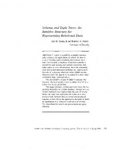
space. As a result, the way that Conficker C constructs a P2P-based botnet is in principle the same as worm scanning/infection. Therefore, characterizing the structure of worm infection is important and imperative for defending against current and future epidemics such as Internet worms and Conficker C like P2P-based botnets. Modeling Internet worm infection has been focused on the macro level. Most, if not all, mathematical models study the total number of infected hosts over time [12, 24, 4, 15, 8]. The models of the micro level of worm infection, however, have been investigated little. The micro-level models can provide more insights into the infection ability of individual compromised hosts and the underlying topologies formed by worm infection. A key micro-level information is “who infects whom” or the worm infection family tree. When a host infects another host, they form a “father-and-son” relationship, which is represented by a directed edge in a graph formed by worm infection. Hence, the procedure of worm propagation constructs a directed tree where patient zero is the root and the infected hosts that do not compromise any vulnerable host are leaves (see Fig. 1). To the best of our knowledge, there is yet no mathematical model for characterizing the structure of such a tree. The goal of this work is to characterize the Internet worm infection family tree, called the “worm tree” in short. For such a tree, we are particularly interested in two metrics: • Number of children: For a randomly selected node in the tree, how many children does it have? This metric represents the infection ability of individual hosts. • Generation: For a randomly selected node in the tree, which generation (or level) does it belong to? This metric indicates the average path length of the graph formed by worm infection. These two metrics have important implications and applications for security analysis. First, the distribution of the number of children can be used to answer questions such as what is the probability that an infected host compromises more than 10 vulnerable hosts. Moreover, it provides insights into the robustness of the Conficker C like P2P-based botnets [1, 7]. Second, some schemes
Generation 3
Section 2 presents our sequential growth model and assumptions used in analyzing the worm tree. Section 3 gives our analysis on the worm tree. Section 4 uses simulations to verify the analytical results. Finally, Section 5 concludes this paper.
Generation 2 Generation 1
2 Worm Tree and Sequential Growth Model
Generation 0 Patient zero
In this section, we provide the background on the worm tree, and present the assumptions and the growth model. An example of a worm tree is given in Fig. 1. Here, patient zero is the root and belongs to generation 0. The tail of an arrow is from the “father” or the infector, whereas the head of an arrow points to the “son” or the infectee. If a father belongs to generation i, then its children lie in generation i + 1. In a worm tree with n nodes, we use Ln (i, j) (0 ≤ i, j ≤ n − 1) to denote the number of nodes that children and belong to generation j. P have Pin−1 Note that n−1 i=0 j=0 Ln (i, j) = n. We also use Cn (i) (i = 0, 1, 2, · · · , n − 1) to denote the number of nodes that have i children and Gn (j) (j = 0, 1, 2, · · · , n − 1) to denote the number of nodes in generation j. Moreover, Ln (i, j), Cn (i), and Gn (j) are random variables. Thus, we define p (i, j) = E[Ln (i,j)] , representing the
Figure 1: A worm tree. have been proposed to trace worms back to their origins through the cooperation between infected hosts [21], and the distribution of the generation can provide the information on the number of hosts required to cooperate. Moreover, it sheds light on the delay or the effort for a botmaster to deliver a command to all bots in a P2Pbased botnet like Conficker C. To study these two metrics analytically, we apply probabilistic modeling methods and derive the joint probability distribution of the number of children and the generation through a sequential growth model. From the joint distribution, we analyze the marginal distributions of the number of children and the generation. We also develop closed-form approximations to both marginal distributions and the joint distribution. As a first attempt, we analyze the worm tree formed by a wide class of worms such as random-scanning worms [12], routable-scanning worms [20, 24], importance-scanning worms [5], OPTSTATIC worms [16], and SUBOPT-STATIC worms [16]. For these worms, a new victim is compromised by each existing infected host with equal probability. We then verify the analytical results through simulations. Through both mathematical analysis and simulation, we make several discoveries from this research as follows. If a worm uses a scanning method for which a new victim is compromised by each existing infected host with equal probability, the number of children is shown to have asymptotically a geometric distribution with parameter 0.5. This means that on average half of infected hosts never compromise any target and over 98% of infected hosts have no more than five children. On the other hand, this also indicates that a small portion of hosts infect a large number of vulnerable hosts. Moreover, the generation is demonstrated to closely follow a Poisson distribution with parameter Hn − 1, where n is the number of nodes and Hn is the n-th harmonic number [6]. This means that the average path length of the worm tree increases approximately logarithmically with the number of nodes. To the best of our knowledge, this is the first attempt in understanding and exploiting the topology formed by worm infection quantitatively. The remainder of this paper is structured as follows.
n
n
joint distribution of the number of children and the generation. Similarly, we define cn (i) = E[Cnn (i)] to represent the marginal distribution of the number of children and gn (j) = E[Gnn (j)] to represent the marginal distribuPn−1 tion of the generation. Note that cn (i) = j=0 pn (i, j) Pn−1 and gn (j) = i=0 pn (i, j). Although we model worm infection as a tree, different worm trees can show very different structures. In the extended version of this paper [18], we demonstrate that two extreme cases of worm trees (i.e., bus and star topologies) can have very different cn (i) and gn (j). To study the worm tree analytically, in this paper we make several assumptions and considerations. First, to simplify the model, we assume that infected hosts have the same scanning rate. This assumption is removed in Section 4.2, where we use simulations to study the effect of the variation of scanning rates on the worm tree. Second, we consider a wide class of worms for which a new victim is compromised by each existing infected host with equal probability. Such worms include randomscanning worms, routable-scanning worms, importancescanning worms, OPT-STATIC worms, and SUBOPTSTATIC worms. Random scanning selects targets in the IPv4 address space randomly and has been the main scanning method for both worms and botnets [12, 10]; routable scanning finds victims in the routable IPv4 address space [20, 24]; and importance scanning probes subnets according to the vulnerable-host distribution 2
[5]. OPT-STATIC and SUBOPT-STATIC are optimal and suboptimal scanning methods that are proposed in [16] to minimize the number of worm scans required to reach a predetermined fraction of vulnerable hosts. Third, we consider the classic susceptible → infected (SI) model, ignoring the cases that an infected host can be cleaned and becomes vulnerable again, or can be patched and becomes invulnerable. The SI model assumes that once infected, a host remains infected. Such a simple model has been widely applied in studying worm infection [12, 24, 16], and presents the worst case scenario. Fourth, we assume that there is no re-infection. That is, if an infected host is hit by a worm scan, this host will not be further re-infected. As a result, every infected host has one and only one father except for patient zero, and the resulting graph formed by worm infection is a tree. Fifth, we assume that the worm starts from one infected host, i.e., patient zero or a hitlist size of 1. When the hitlist size is larger than 1, the underlying infection topology is a worm forest, instead of a worm tree. Our analysis, however, can easily be extended to model the worm forest. Finally, we assume that in our model, nodes are added into the worm tree sequentially and no two nodes are added at the same time. That is, no two vulnerable hosts are infected simultaneously. Rather than attempting to characterize the dynamics of worm propagation (e.g., the total number of infected hosts over time), we make this assumption aim at capturing the main features of the topology formed by worm infection (e.g., the number of children and the generation) without sacrificing much accuracy. Taking the Code Red v2 worm as an example, during its early stage of propagation, there are few infected hosts struggling to find other vulnerable machines out of the IPv4 address space, hence very few hosts get infected at the same time. On the other hand, during its later fast spread period, the number of hosts that get compromised simultaneously is trivial compared with the number of existing infected hosts. In Section 4 where simulations are performed, we relax this assumption.
paper, we apply this model to characterize worm infection.
3 Mathematical Analysis In this section, we study the worm tree through mathematical analysis. Specifically, we first derive the joint distribution of the number of children and the generation, i.e., pn (i, j), by applying probabilistic methods. We then use pn (i, j) to analyze two marginal distributions, i.e., cn (i) and gn (j), and obtain their closed-form approximations. Finally, we find a closed-form approximation to pn (i, j).
3.1 Joint Distribution For a worm tree with only patient zero (i.e., n = 1), since L1 (0, 0) = 1 with probability 1, p1 (0, 0) = 1. Similarly, for a worm tree with n = 2, it is evident that L2 (1, 0) = L2 (0, 1) = 1. Thus, p2 (1, 0) = p2 (0, 1) = 12 . We now consider pn (i, j) (0 ≤ i, j ≤ n − 1) when n ≥ 3. Specifically, we study two cases: (1) pn (0, j), i.e., the proportion of the number of leaves in generation j in Tn . Assume that Tn−1 is given, and there are Ln−1 (0, j) leaves in generation j and toPn−2 tally Gn−1 (j −1) = i=0 Ln−1 (i, j − 1) nodes in generation j − 1. Note that we have extended the notation so that Gn−1 (−1) = Ln−1 (i, −1) = 0, 0 ≤ i ≤ n − 2. When a new node vn is added, vn becomes a leaf of Tn . If vn is connected to one of existing nodes in generation j − 1, vn belongs to generation j; and the probability of (j−1) such an event is Gn−1 . Moreover, if a leaf in genn−1 eration j in Tn−1 connects to vn , this node is no longer a leaf and now has one child; and the probability of this (0,j) event is Ln−1 . Therefore, we can obtain the stochasn−1 tic recurrence of Ln (0, j): Gn−1 (j−1) Ln−1 (0, j) + 1, w.p. n−1 (0,j) Ln (0, j) = Ln−1 (0, j) − 1, w.p. Ln−1 n−1 Ln−1 (0, j), otherwise.
(1) Given Tn−1 (i.e., Ln−1 (0, j) and Gn−1 (j − 1)), the conditional expected value of Ln (0, j) is [Ln−1 (0, j) + 1] · Gn−1 (j−1) (0,j) + [Ln−1 (0, j) − 1] · Ln−1 + Ln−1 (0, j) · n−1 h n−1 i Gn−1 (j−1)+Ln−1 (0,j) 1− , i.e., n−1
Based on these considerations and assumptions, the sequential growth model of a worm tree works as follows: We consider a fixed sequence of infected hosts (i.e., nodes) v1 , v2 , · · · and inductively construct a random worm tree (Tn )n≥1 , where n is the number of nodes and T1 has only patient zero. Infecting a new host is equivalent to adding a new node into the existing worm tree. Hence, given Tn−1 , Tn is formed by adding node vn together with an edge directed from an existing node vf to vn . According to the assumption, vf is randomly chosen among the n − 1 nodes in the tree, i.e., 1 Pr(f = k) = n−1 , k = 1, 2, · · · , n − 1. Note that such a sequential growth model and its variations have been widely used in studying topology generators [2]. In this
E[Ln (0, j)|Tn−1 ] =
n−2 1 n−1 Ln−1 (0, j)+ n−1 Gn−1 (j −1).
(2) Applying E[Ln (0, j)] = E[E[Ln (0, j)|Tn−1 ]] (i.e., the law of total expectation), we obtain E[Ln (0, j)] =
n−2 1 n−1 E[Ln−1 (0, j)] + n−1 E[Gn−1 (j − 1)].
(3) E [Ln (0,j)] Using the definitions pn (0, j) = and gn−1 (j − n Pn−2 E [Gn−1 (j−1)] 1) = = i=0 pn−1 (i, j − 1), the above n−1 3
Moreover, note that c2 (0) = 12 . If we assume that cn−1 (0) = 12 , we can obtain by induction that
equation leads to pn (0, j) = =
n−2 n pn−1 (0, j) n−2 n pn−1 (0, j)
+ n1 gn−1 (j − 1) (4) P n−2 + n1 i=0 pn−1 (i, j − 1).
cn (0) = 21 .
This indicates that no matter how many nodes are in the worm tree, on average half of nodes are leaves, i.e., on average 50% of infected hosts never compromise any target. (2) cn (i), 1 ≤ i ≤ n − 1. From Equation (9) and Pn−1 cn (i) = j=0 pn (i, j), we find the recurrence of cn (i) as follows
(5)
(2) pn (i, j), 1 ≤ i ≤ n − 1. Given Ln−1 (i, j) and Ln−1 (i − 1, j) in Tn−1 , we study Ln (i, j) in Tn . When the new node vn is added into Tn−1 , vn is connected to a node with i − 1 children and in generation j with (i−1,j) probability Ln−1n−1 , or is connected to a node with i (i,j) . children and in generation j with probability Ln−1 n−1 Thus, in Tn , Ln−1 (i−1,j) Ln−1 (i, j) + 1, w.p. n−1 (i,j) Ln (i, j) = Ln−1 (i, j) − 1, w.p. Ln−1 n−1 Ln−1 (i, j), otherwise. (6) This relationship leads to
E[Ln (i, j)|Tn−1 ] =
cn (i) =
n−2 1 n−1 Ln−1 (i, j)+ n−1 Ln−1 (i−1, j).
(8)
Corollary 1 When n ≥ 1, the expectation and the variance of the number of children are Pn−1 En [C] = i=0 i · cn (i) = n−1 (15) n
That is, + n1 pn−1 (i − 1, j).
(9)
Summarizing the above two cases, we have the following theorem:
3.2 Number of Children
The proof of Corollary 1 is given in the extended version of this paper [18]. One intuitive way to derive En [C] is that in worm tree Tn , there are n − 1 directed edges and n nodes. Thus, the average number of edges (i.e, the average number of children) of a node is n−1 n . Moreover, since Hn is O(1 + ln n), lim En [C] = 1, and n→∞
Corollary 2 When n → ∞, the number of children has a geometric distribution with parameter 12 , i.e., � 1 �i+1 , i = 0, 1, 2, · · · . (17) c(i) = lim cn (i) = n→∞ 2
We use pn (i, j) to derive the marginal distribution of the number of children, i.e., cn (i). Similarly, we study two cases: (1) cn (0), i.e., the proportion of the number of Pn−1 leaves in Tn . Since cn (0) = j=0 pn (0, j) and Pn−1 j=0 gn−1 (j − 1) = 1, we obtain the recursive relationship of cn (0) from Equation (4): + n1 .
2
i=0
lim Varn [C] = 2. n→∞ Theorem 2 also leads to a simple closed-form expression of the distribution of the number of children when n is very large, as shown in the following corollary.
Theorem 1 provides a way to calculate pn (i, j) recursively from p2 (i, j).
n−2 n cn−1 (0)
Pn−1
2Hn (i − En [C]) · cn (i) = 2− n−1 n2 − n , (16) P where Hn = ni=1 1i is the n-th harmonic number [6].
Varn [C] =
Theorem 1 When n ≥ 3, the joint distribution of the number of children and the generation in a worm tree Tn follows ( n−2 1 n pn−1 (0, j) + n gn−1 (j − 1), i = 0 pn (i, j) = n−2 1 n pn−1 (i, j) + n pn−1 (i − 1, j), otherwise, (10) where 0 ≤ i, j ≤ n − 1.
cn (0) =
(13)
From Theorem 2, we can derive the statistical properties of the number of children as follows.
n−2 1 n−1 E[Ln−1 (i, j)]+ n−1 E[Ln−1 (i−1, j)].
n−2 n pn−1 (i, j)
+ n1 cn−1 (i − 1).
Theorem 2 When n ≥ 3, the distribution of the number of children in a worm tree Tn follows ( 1 i=0 2, cn (i) = n−2 1 n cn−1 (i) + n cn−1 (i − 1), 1 ≤ i ≤ n − 1. (14)
(7)
pn (i, j) =
n−2 n cn−1 (i)
Summarizing the above two cases, we have the following theorem on the distribution of the number of children:
Therefore, E[Ln (i, j)] =
(12)
The proof of Corollary 2 is given in [18]. Corollary 2 indicates that when n is very large, cn (i) decreases approximately exponentially with a decay constant of ln 2 as the number of children increases. We further study when both n and i are finite and large, how cn (i) varies
(11) 4
Analysis (n = 1000) Poisson (λn = H1000 − 1) Analysis (n = 2000) Poisson (λn = H2000 − 1) Analysis (n = 5000) Poisson (λn = H5000 − 1) Analysis (n = 20000) Poisson (λn = H20000 − 1)
0.01
0.12
gn (j)
cn (i)
1.0E−4
1.0E−6
1.0E−8
1.0E−10
1.0E−12 0
Analysis (n = 1000) Analysis (n = 2000) Analysis (n = 5000) Analysis (n = 20000) Geometric 5
10
0.06
15
20
25
0 0
5
Number of children (i)
(a) Number of children.
10
15
20
25
0.08
Approximated joint distribution
0.18
0.5
0.07 0.06 0.05 0.04 0.03 0.02 0.01
30
Generation (j)
0 0
0.02
0.04
0.06
0.08
Actual joint distribution
(c) Joint distribution (n = 2000).
(b) Generation.
Figure 2: Mathematical analysis of the worm infection structure. with n, i.e., how the tail of the distribution of the number of children changes with n. First, note that c3 (0) = 21 , c3 (1) = 13 , and c3 (2) = 16 . Thus, from Equation (13), we can prove by induction that cn (i) (n ≥ 3) is a decreasing function of i, i.e., cn (i) < cn (i − 1), for 1 ≤ i ≤ n − 1. Next, putting this inequality into Equation (13), we have cn (i) > n−1 n cn−1 (i). Hence, when n is very large, n−1 ≈ 1, and cn (i) > cn−1 (i), which n indicates that the tail of cn (i) increases with n. Fig. 2(a) verifies this result, showing cn (i) obtained from Theorem 2 when n = 1000, 2000, 5000, and 20000, as well as the geometric distribution with parameter 0.5 obtained from Corollary 2. Note that the y-axis uses log-scale. It can be seen that when n increases from 1000 to 20000, the tail of cn (i) also increases to approach the tail of the geometric distribution. Moreover, it is shown that the geometric distribution well approximates the distribution of the number of children when n is large.
ance of the generation are Pn−1 En [G] = j=0 j · gn (j) = Hn − 1.
(19)
(j − En [G])2 · gn (j) = Hn − Hn,2 , (20) Pn Pn where Hn = i=1 1i and Hn,2 = i=1 i12 . Varn [G] =
Pn−1 j=0
The proof of Corollary 3 is given in [18]. From Corollary 3, we have some interesting observations. Since Hn 2 is O(1 + ln n) and H∞,2 = ζ(2) = π6 ≈ 1.645 is the Riemann zeta function of 2 [13], both En [G] and Varn [G] are O(1 + ln n). This indicates that the average path length of the worm tree (i.e., En [G]) increases approximately logarithmically with n. Moreover, when n → ∞, lim En [G] − ln n = γ − 1, and lim Varn [G] − ln n = n→∞
n→∞
γ − ζ(2), where γ ≈ 0.577 is the Euler-Mascheroni constant [9]. Therefore, when n is large, En [G] ≈ Varn [G]. Furthermore, we can use Theorem 3 to obtain a closedform approximation to gn (j) as follows.
3.3 Generation
Corollary 4 When n is very large, the generation distribution gn (j) can be approximated by a Poisson distribution with parameter λn = En [G] = Hn − 1. That is,
Next, we derive the generation distribution (i.e., gn (j)) in a similar manner to the case of cn (i). Using Theorem Pn−1 1 and gn (j) = i=0 pn (i, j), we obtain the following theorem:
gn (j) ≈
Theorem 3 When n ≥ 3, the distribution of the generation in a worm tree Tn follows
λjn −λn , j! e
0 ≤ j ≤ n − 1.
(21)
+ n1 gn−1 (j − 1), 0 ≤ j ≤ n − 1, (18)
The proof of Corollary 4 is given in [18]. Fig. 2(b) verifies Corollary 4, showing gn (j) obtained from Theorem 3 when n = 1000, 2000, 5000, and 20000, as well as the Poisson distribution with parameter En [G]. It can be seen that when n is large, the Poisson distribution fits the generation distribution closely.
Theorem 3 gives a method to calculate the distribution of the generation recursively. Moreover, from Theorem 3, we can derive the statistical properties of the generation distribution in the following corollary.
3.4 Approximation to the Joint Distribution
gn (j) =
n−1 n gn−1 (j)
where gn−1 (−1) = 0.
Finally, we derive a closed-form approximation to the joint distribution pn (i, j). From Equation (9), we can see
Corollary 3 When n ≥ 1, the expectation and the vari5
0.15
Simulation (n = n0 /4) Simulation (n = n0 ) Simulation (n = 4n0 ) Geometric
0.01
Simulation (n = n0 /4) Simulation (n = n0 ) Simulation (n = 4n0 ) Poisson (λn = Hn0 /4 − 1) Poisson (λn = Hn0 − 1) Poisson (λn = H4n0 − 1)
gn (j)
cn (i)
0.1
1.0E−4
0.05
1.0E−6
0.06
Approximated joint distribution
0.5
0.05 0.04 0.03 0.02 0.01
1.0E−8 0
5
10
15
20
25
0 0
5
10
15
20
Number of children (i)
Generation (j)
(a) Number of children.
(b) Generation.
25
30
35
0 0
0.02
0.04
0.06
Measured joint distribution
(c) Joint distribution (n = n0 ).
Figure 3: Simulating the infection structure of the Code Red v2 worm (n0 = 360, 000). that when n → ∞, pn (i, j) = pn−1 (i, j), which yields pn (i, j) =
1 2 pn (i
Hence, we can obtain �i pn (i, j) = 21 pn (0, j) ≈
− 1, j). � 1 i+1 gn (j). 2
the simulator is not based on any mathematical model. Instead, the simulator considers a discrete-time system and mimics the random-scanning behavior of infected hosts in real world scenarios through a random number generator. Moreover, the parameter setting is based on the Code Red v2 worm’s characteristics. For example, the vulnerable population is n0 = 360, 000, and a newly infected host is assigned with a scanning rate of 358 scans/min. Detailed information about how the parameters are chosen can be found in Section VII of [23]. We then extend the simulator to track the worm infection structure by adding the information of the number of children and the generation to each infected host. Moreover, we set the discrete time unit to 20 seconds and start our simulation at time tick 0 with patient zero. Note that we remove the assumption used in the sequential growth model that no two hosts are compromised at the same time. That is, multiple hosts can be compromised at one time tick. Moreover, all new victims of the current time tick start scanning at the next time tick. The simulation results (mean ± standard deviation) are obtained from 100 independent runs with different seeds and are presented in Fig. 3. Fig. 3(a) shows the distribution of the number of children, comparing the simulation results of cn (i) for n = n0 /4, n0 , and 4n0 with the geometric distribution obtained from Corollary 2. Note that the y-axis uses the log-scale. The vertical dotted line represents the standard deviation that goes into the negative territory. It can be seen that the distribution of the number of children can be well approximated by the geometric distribution with parameter 0.5. This implies that cn (i) decreases approximately exponentially with a decay constant of ln 2. Specifically, in all three cases, on average 50.0% of the infected hosts do not have children, about 98.4% of them have no more than five children, and 0.1% of them have no less than ten children. We also calculate the expectation and the variance of the number of children from the simulation and find that they are identical to the analyti-
(22)
(23)
Since when n is very large, gn (j) follows closely the Poisson distribution as in Corollary 4, �i+1 λj −λ · j!n e n , 0 ≤ i, j ≤ n − 1, (24) pn (i, j) ≈ 12
where λn = Hn − 1. The above derivation also shows that when n is very large, the number of children and the generation are almost independent random variables. Fig. 2(c) shows the parity plot of the approximation to the joint distribution when n = 2000. In the figure, the x-axis is the actual pn (i, j) obtained from Theorem 1, and the y-axis is the approximated pn (i, j) from Equation (24), where 0 ≤ i, j ≤ 30. It can be seen that most points are on or near the diagonal line, indicating that the approximation to the joint distribution is reasonable.
4 Simulations and Verification In this section, we study the worm infection structure through simulations. As far as we know, there is no publicly available data to show the real worm tree and verify our analytical results. Moreover, real experiments in a controlled environment are impractical for this study, since the closed-form approximations are derived based on the assumption that the number of nodes is very large. Therefore, we apply simulations. Specifically, we first simulate the infection structure of the Code Red v2 worm and then study the effects of important parameters on the worm tree.
4.1 Code Red v2 Worm Verification We simulate the propagation of the Code Red v2 worm by using and extending the simulator in [22]. Note that 6
0.5
0.15
Simulation (s = 158) Simulation (s = 358) Simulation (s = 558) Geometric
0.01
0.5
Simulation (s = 158) Simulation (s = 358) Simulation (s = 558) Poisson (λn = Hn0 − 1)
1.0E−4
cn (i)
gn (j)
cn (i)
0.1
1.0E−4
Simulation (σ = 0) Simulation (σ = 100) Simulation (σ = 200) Geometric
0.01
1.0E−6 1.0E−8
0.05
1.0E−6
1.0E−10
0
5
10
15
20
0 0
25
5
10
Number of children (i)
(a) Effect of s on cn (i). 0.15
15
20
25
30
1.0E−12 0
35
10
Generation (j)
(b) Effect of s on gn (j). 0.5
Simulation (σ = 0) Simulation (σ = 100) Simulation (σ = 200) Poisson (λn = Hn0 − 1)
0.15
0.1 gn (j)
cn (i)
40
Simulation (hitlist = 1) Simulation (hitlist = 10) Simulation (hitlist = 100) Poisson (λn = Hn0 − 1) Poisson (λn = Hn0 /10 − 1) Poisson (λn = Hn0 /100 − 1)
0.1
gn (j)
30
(c) Effect of σ on cn (i).
Simulation (hitlist = 1) Simulation (hitlist = 10) Simulation (hitlist = 100) Geometric
0.01
20
Number of children (i)
1.0E−4
0.05
0.05 1.0E−6
0
5
10
15 20 Generation (j)
25
30
(d) Effect of σ on gn (j).
0
5
10
15
20
Number of children (i)
(e) Effect of hitlist sizes on cn (i).
0 0
5
10
15 20 Generation (j)
25
30
(f) Effect of hitlist sizes on gn (j).
Figure 4: Effects of the scanning rate, the scanning rate standard deviation, and the hitlist size on cn (i) and gn (j) (n0 = 360, 000). dent simulation runs and are shown in Fig. 4. Fig.s 4(a) and (b) show the effect of varying the scanning rate s (scans/min) from 158 to 558 on the distributions of the number of children and the generation. Here, the scanning rate is set to a fixed value for every infected host, i.e., the scanning rate standard deviation is 0. The figures also plot the geometric distribution with parameter 0.5 and the Poisson distribution with parameter Hn0 −1 for reference. It can be seen that the scanning rate does not affect the worm tree structure. Fig.s 4(c) and (d) demonstrate the effect of the variation of the scanning rates among different hosts (i.e., σ). In our simulation, a newly infected host is assigned with a scanning rate (scans/min) from a normal distribution N (358, σ 2 ). The figures show the simulation results when σ = 0, 100, and 200. It can be seen that while the scanning rate standard derivation σ has no effect on the generation distribution, it does affect the distribution of the number of children. Specifically, when σ increases, the tail of cn (i) moves upward from the geometric distribution with parameter 0.5. This is because when σ becomes larger, the variation of the scanning rate among infected hosts is greater. That is, there are more hosts with high scanning rates and also more hosts with low scanning rates. As a result, those hosts with high scanning rates tend to infect a large number of hosts, making
cal results obtained from Corollary 1. Fig. 3(b) demonstrates the generation distribution, comparing the simulation results of gn (j) for n = n0 /4, n0 , and 4n0 with the Poisson distributions with parameter En [G] = Hn −1 obtained from Corollary 4. It can be seen that the simulation results of gn (j) closely follow the Poisson distributions for all three cases. Hence, simulation results verify that the average path length of the worm tree increases approximately logarithmically with the total number of infected hosts. Moreover, we also compute the expectation and the variance of the generation in simulations and verify the analytical results in Corollary 3. Fig. 3(c) compares the measured joint distribution from simulations with the approximated joint distribution from Equation (24) by using the parity plot. It can be seen that most points are on or near the diagonal line, indicating that the approximation works well.
4.2 Effects of Worm Parameters Next, we extend our simulator to examine the effects of three important parameters of worm propagation on the worm tree: the scanning rate, the scanning rate standard deviation, and the hitlist size. When a parameter is studied and varied, we set other parameters to the parameters of the Code Red v2 worm as used in Section 4.1. The simulation results are obtained from 100 indepen7
the tail of cn (i) move upward. However, it is also observed that when σ is not very large (the case for real worms), the geometric distribution with parameter 0.5 is still a good approximation. In Fig.s 4(e) and (f), we show the effect of the hitlist size on the worm tree. As pointed out in Section 2, when the hitlist size is greater than 1, the underlying infection topology is a worm forest with the number of trees equal to the hitlist size. Moreover, in a worm forest, it is intuitive that each tree is a smaller version of the single worm tree of hitlist size 1 and has fewer nodes. Hence, it is not surprising to see that in Fig. 4(f), the generation distribution moves leftward when the hitlist size increases. However, the generation distribution can still be well approximated by the Poisson distribution with parameter Hnh − 1, where nh is the average number of nodes in a tree. Moreover, since in each tree the distribution of the number of children can be approximated by the geometric distribution with parameter 0.5, in the worm forest cn (i) still follows closely the same distribution.
[4] C HEN , Z., G AO , L., AND K WIAT, K. Modeling the Spread of Active Worms. In Proc. IEEE INFOCOM (Apr. 2003). [5] C HEN , Z., AND J I , C. Optimal Worm-Scanning Method Using Vulnerable-Host Distributions. International Journal of Security and Networks (IJSN): Special Issue on Computer and Network Security 2, 1/2 (2007), 71 – 80. [6] C ORMEN , T. H., L EISERSON , C. E., R IVEST, R. L., S TEIN , C. Introduction to Algorithms (Second Edition). The MIT Press and McGraw-Hill (2002). [7] D AGON , D., G U , G., L EE , C., AND L EE , W. A Taxonomy of Botnet Structures. In Proc. 23 Annual Computer Security Applications Conference (ACSAC’07) (Dec. 2007). [8] D AGON , D., Z OU , C. C., AND L EE , W. Modeling Botnet Propagation Using Time Zones. In Proc. NDSS (Feb. 2006). [9] H AVIL , J. Gamma: Exploring Euler’s Constant. Princeton University Press (2003). [10] L I , Z., G OYAL , A., C HEN , Y., AND PAXSON , V. Automating Analysis of Large-Scale Botnet Probing Events. In Proc. ACM Symposium on Information, Computer and Communication Security (ASIACCS’09) (Mar. 2009). [11] P ORRAS , P., S AIDI , H., AND Y EGNESWARAN , V. Conficker C P2P Protocol and Implementation. SRI International Technical Report (Sept. 2009). [12] S TANIFORD , S., PAXSON , V., AND W EAVER , N. How to 0wn the Internet in your spare time. In Proc. 11th USENIX Security Symposium (Security’02) (Aug. 2002).
5 Conclusions In this paper, we attempt to capture the key characteristics of the Internet worm infection family tree. We have analyzed the infection tree formed by a wide class of worms such as random-scanning worms, routablescanning worms, importance-scanning worms, OPTSTATIC worms, and SUBOPT-STATIC worms. Through both mathematical analysis and simulation, we have shown that the number of children asymptotically has a geometric distribution with parameter 0.5; and the generation closely follows a Poisson distribution with parameter En [G] (i.e., Hn − 1). As part of our ongoing work, we plan to relax our assumptions to include more worm dynamics and apply our observations to botnets. For example, we are studying the infection structure of localized scanning [18], and effect of user defenses and re-infection on the worm tree [19]. Moreover, based on our observations, we are developing methods for detecting bots and studying potential countermeasures for a botnet (e.g., Conficker C) that uses scan-based peer discovery to form a P2P-based botnet [18].
[13] T ITCHMARSH , E. C. The Theory of the Riemann Zeta Function. Oxford University Press (1986). [14] V OGT, R., AYCOCK , J., AND M. JACOBSON , J. Army of Botnets. In Proc. NDSS (Feb. 2007). [15] V OJNOVIC , M., AND G ANESH , A. J. On the Race of Worms, Alerts and Patches. IEEE/ACM Transactions on Networking 16, 5 (Oct. 2008), 1066–1079. [16] V OJNOVIC , M., G UPTA , V., K ARAGIANNIS , T., AND G KANTSIDIS , C. Sampling Strategies for Epidemic-Style Information Dissemination. to appear in IEEE/ACM Transactions on Networking. [17] WANG , P., S PARKS , S., AND Z OU , C. C. An Advanced Hybrid Peer-to-Peer Botnet. IEEE Transactions on Dependable and Secure Computing 7, 2 (Apr.-Jun. 2010), 113–127. [18] WANG , Q., C HEN , Z., AND C HEN , C. Charaterizing Internet Worm Infection Structure. Preprint. [Online]. Available: http: //arxiv.org/abs/1001.1195. [19] WANG , Q., C HEN , Z., C HEN , C., AND P ISSINOU , N. On the Robustness of the Botnet Topology Formed by Worm Infection. In Proc. IEEE GLOBECOM (Dec. 2010). [20] X IA , J., VANGALA , S., J. W U , L. G., AND K WIAT, K. Effective Worm Detection for Various Scan Techniques. Journal of Computer Security 14, 4 (2006), 359 – 387. [21] X IE , Y., S EKAR , V., M ALTZ , D. A., R EITER , M. K., AND Z HANG , H. Worm Origin Identification Using Random Walks. In Proc. IEEE Symposium on Security and Privacy (May 2005).
References
[22] Z OU , C. C. Internet Worm Propagation Simulator. [Online]. Available: http://www.cs.ucf. edu/˜czou/research/wormSimulation/ simulator-codered-100run.cpp.
´ , A.-L. Statistical Mechanics of [1] A LBERT, R., AND BARAB ASI Complex Networks. Review of Modern Physics 74 (2002), 47– 97. ´ , A.-L., AND A LBERT, R. Emergence of Scaling in [2] BARAB ASI Random Networks. Science 286 (Oct. 1999), 509–512.
[23] Z OU , C. C., G ONG , W., T OWSLEY, D., AND G AO , L. The Monitoring and Early Detection of Internet Worms. IEEE/ACM Transactions on Networking 13, 5 (Oct. 2005), 967–974.
[3] CAIDA. Conficker/Conflicker/Downadup as seen from the UCSD Network Telescope. [Online]. Available: http://www.caida.org/research/security/ ms08-067/conficker.xml.
[24] Z OU , C. C., T OWSLEY, D., AND G ONG , W. On the Performance of Internet Worm Scanning Strategies. Elsevier Journal of Performance Evaluation 63, 7 (Jul. 2006), 700–723.
8