Electronic Supplementary Information - Part Two. Chloride ..... 17 CHARMM-GUI. http://www.charmm-gui.org/?doc=input/membrane (2011). 18 N. KuÄerka, M.-P.
Electronic Supplementary Material (ESI) for Chemical Science This journal is © The Royal Society of Chemistry 2012
Electronic Supplementary Information - Part Two
Chloride,
carboxylate
and
carbonate
transport
by
ortho-
phenylenediamine-based bisureas Stephen J. Moore,a Cally J. E. Haynes,a Jorge González, a,b Jennifer L. Sutton,a Simon J. Brooks,a Mark E. Light,a Julie Herniman,a G. John Langley,a Vanessa Soto-Cerrato,c Ricardo Pérez-Tomás,c Igor Marques,d Paulo J. Costa,d Vítor Félixd and Philip A. Gale*a
Computational Details with Extended Results The molecular mechanics calculations (MM) and molecular dynamics (MD) simulations were performed with AMBER12 suite.6 The Gaussian09 package was used for all electronic structure calculations.7 MM and MD modelling studies were undertaken with receptors 1-11 described by the general Amber force field (GAFF)8 and atomic RESP charges,9 which were determined as explained below. In the chloride complexes, the anion was described with a net charge set to -1 and van der Waals parameters10 developed for the TIP3P water model.11 The hydrogen carbonate anion was also described with parameters taken from GAFF and RESP atomic charges. The TIP3P water model was employed in water solution and POPC bilayer simulations, which were both carried out under periodic boundary conditions. The charge neutrality of membrane model systems was attained by the addition of a sodium counter-ion with a net charge of +1 and van der Waals parameters for TIP3P.10 The LIPID11 force field parameters were for the individual POPC lipids.12 RESP charge calculations The atomic point charges of compounds 1-11 were obtained by means of a multiconformational RESP charge fitting methodology.9 Initially, transporters 1-11 were geometry optimized at the HF/6-31G* level of theory using Gaussian09 with a random starting conformation. Subsequently, the RESP atomic charges for this single conformation were fitted to the electrostatic potential (ESP) computed at the HF/6-31G* using 4 concentric layers of points per atom and 6 points per unit area (Gaussian IOp(6/42=6)) in agreement with the methodology followed in the force field reference. Parameters taken from GAFF were assigned to 1-11, which were then submitted to a 1 ns MD quenched run in the gas phase at 1000 K using the sander module from AMBER12, which allowed a stochastic covering of the conformational space of the transporters. A trajectory file composed of 10000 structures was saved, which were further full MM minimized until the convergence criterion of 0.0001 kcal mol-1 was S 80
Electronic Supplementary Material (ESI) for Chemical Science This journal is © The Royal Society of Chemistry 2012
achieved. Afterwards, the conformations of each molecule were energy sorted and also clustered by root-mean-square deviation (RMSD). In order to obtain charges less dependent of the molecular conformation, five different conformations were selected for 1-8 according to the possible configurations of the urea binding units with 2 syn/syn structures, 2 syn/anti structures and 1 anti/anti structure. The lowest energy conformation was always among the selected structures. For monoureas 9-11, five conformations with anti or syn urea arrangements were also considered following an equivalent criterion. These 5 conformations were again geometry optimized at the HF/6-31G* level of theory and the electrostatic potential was calculated for each of them, allowing the calculation of multi-conformational RESP atomic point charges, using identical weights for all conformations. The determination of the RESP atomic charges of HCO3- anion was carried out with a single structure using the Gaussian IOp aforementioned. The structures of 1-11 chloride complexes as well as 5•HCO3- were obtained via quenched MD simulations as described above for free compounds 1-11. Simulation of 1-11 in water solution towards the surface area calculations Suitable structures of 1-11 with syn/syn, syn/anti and anti/anti conformations (three urea arrangements for 1-8 and two for 9-11) were immersed in cubic boxes containing a variable number of TIP3P water molecules ranging between 2068 and 3215. Subsequently these solvated systems were subject to the following multi-stage equilibration protocol. The solvent was relaxed by a MM minimization with a harmonic restraint of 500 kcal mol-1 Å-2 on the receptors, followed by a MM minimization of all system. The system was then heated to 300 K during 50 ps using the Langevin thermostat with a collision frequency of 1 ps-1 in an NVT ensemble. Afterwards the density of the system was adjusted for 1 ns in a NPT ensemble at 1 atm with isotropic pressure scaling using a relaxation time of 1 ps, followed by a production run of 10 ns. The SHAKE13 algorithm was used to constrain all bonds involving hydrogen atoms, allowing the usage of a 2 fs time step. An 8 Å cut-off was used for the van der Waals and non-bonded electrostatic interactions. Frames were saved every 1.0 ps leading to a trajectory files containing 10000 structures for each receptor in each conformation. These simulations were performed with pmemd.cuda AMBER12 executable, which
S 81
Electronic Supplementary Material (ESI) for Chemical Science This journal is © The Royal Society of Chemistry 2012
allowed to accelerate explicit solvent Particle Mesh Ewald (PME) calculations14 through the use of GPUs.15 The Polar Surface Area (PSA) was calculated taking into account only the polar atoms non carbon atoms and the hydrogen atoms attached to them using the Linear Combinations of Pairwise Overlaps (LCPO) algorithm16 implemented in the cpptraj utility of Ambertools 12.6 All molecules preserved the corresponding binding units’ configuration along the entire simulation time and therefore all saved frames were used to estimate the average values of PSA and Total Surface Area (TSA) parameters, collected in Table S1. Table S1. PSA and TSA (Å2)a for receptors 1-11 in the different representative conformations. Parameter Configuration
TSA
1
syn/syn 89.9 ± 7.1
syn/anti 94.6 ± 5.2
anti/anti syn/syn 98.0 ± 5.9 482.7 ± 18.0
syn/anti 459.6 ± 18.6
anti/anti 464.3 ± 15.9
2
155.5 ± 6.0
158.5 ± 5.1
163.6 ± 5.8 484.6 ± 17.9
474.8 ± 17.6
467.6 ± 15.9
3
198.9 ± 6.7
201.8 ± 5.8
205.6 ± 5.9 530.0 ± 17.9
519.5 ± 18.2
510.9 ± 15.4
203.6 ± 8.4
204.9 ± 7.0
201.6 ± 6.6 564.3 ± 23.2
547.8 ± 25.8
507.3 ± 24.1
5
271.8 ± 11.9 273.9 ± 11.3
262.4 ± 12.6 601.8 ± 28.4
596.4 ± 29.2
553.0 ± 27.4
6
286.0 ± 12.4 255.9 ± 13.6
272.9 ± 15.6 565.0 ± 27.1
497.8 ± 21.5
517.2 ± 31.6
7
263.4 ± 27.6 248.5 ± 19.4
255.8 ± 15.8 544.6 ± 40.4
510.9 ± 22.2
508.5 ± 18.3
8
203.0 ± 21.7 196.8 ± 18.3
215.6 ± 14.7 520.1 ± 21.8
4
a
PSA b
9
114.1 ± 1.3
10
150.2 ± 1.5
515.3 ± 15.7
509.0 ± 12.6
-
119.5 ± 1.2 392.9 ± 2.9
-
392.7 ± 2.8
-
155.4 ± 1.4
-
414.2 ± 3.0
415.1 ± 3.0
157.5 ± 1.5 162.9 ± 1.4 396.4 ± 2.9 396.1 ± 2.9 11 The value of both parameters are given as A ± SD, being A the average value and SD the corresponding
standard deviation.; b Configuration defined by the two thiourea binding units.
Correlations were sought between the calculated TSA and PSA values with the activities (EC50,
270 s
values). The clogP values were also analysed and, in fact, the
activity does not appear to be correlated with the clogP values (see Figure S94, top left) whereas the PSA appears to be mildly correlated with the activity: higher PSA values lead to larger activities (Figure S94, top right). The correlation appears to be improved when the TSA values are considered, and, as a general trend, as the TSA increases, the activity also increases (Figure S94, bottom).
S 82
Electronic Supplementary Material (ESI) for Chemical Science This journal is © The Royal Society of Chemistry 2012
Figure S94. Plot of the calculated octanol:water partition coefficients, clogP (top left), PSA (top right) and TSA (bottom) as a function of the experimental EC50 270 s values. For the PSA and TSA values, only the syn/syn values were considered.
S 83
Electronic Supplementary Material (ESI) for Chemical Science This journal is © The Royal Society of Chemistry 2012
Membrane/transporter systems setup and simulation protocol A previously equilibrated bilayer, composed of 128 POPC lipid molecules (64 lipids per monolayer) was obtained from the CHARMM membrane builder17 and hydrated to a total of 6500 TIP3P water molecules.11 5•Cl-, 6•Cl-, 5•HCO3- complexes were immersed in the water slab, away (>8 Å) from the water/lipid interface, along with a Na+ counter-ion for charge neutrality The systems were relaxed by MM using 3000 steps of steepest descent plus 7000 steps of conjugate gradient minimization with a large harmonic restraint (500 kcal/mol Å2) on the complexes in order to remove bad contacts between the water molecules and the complexes and, then, a full MM minimization was performed to all systems. After the minimization, a short NVT MD run of 50 ps at 303 K was performed keeping a weak 10 kcal/mol Å2 restraint on the complexes. In order to keep the bilayer membrane structure, the POPC lipids were also restrained in the first MM and NVT stages using the same harmonic positional restraints. The equilibration process followed in an NPγT ensemble run for 20 ns using a surface tension (γ) of 17 dyn cm-1 and keeping the weak positional restraint only on the complexes. Then, this restraint was removed and each system was subject to an 80 ns production run. The snapshots of 5•Cl- and 6•Cl- shown in Figure S95 illustrate the system configurations prior to the 80 ns production runs. Two replicates were produced for each system using different seeds to the velocities generation in the NVT stage. The non-bonded interactions were truncated with an 8 Å cut-off. The long-range electrostatic interactions were described with PME.14 The temperature of the system was maintained by coupling the system to an external bath temperature of 303 K, using the Langevin thermostat with a coupling constant of 0.1 ps-1. The pressure was controlled by the Berendsen barostat at 1 atm (coupling constant of 1.0 ps) and using a compressibility of 44.6×10⁻⁶ bar-1. The covalent bonds to hydrogen atoms were constrained using the SHAKE algorithm13 allowing the use of a 2 fs time step length. The membrane simulations were also performed with the CUDA versions of PMEMD executable.15 The membrane structural parameters were analysed with the cpptraj tool and house made scripts.
S 84
Electronic Supplementary Material (ESI) for Chemical Science This journal is © The Royal Society of Chemistry 2012
Supporting Figures for membrane simulations
Figure S95. Snapshots of systems 5•Cl- (left) and 6•Cl- (right) after the multi-stage equilibration process and prior to the 80 ns MD simulation run.
Figure S96. Hydrogen bonds counting for the N-H···O=P bonding interactions between 5 (top, for the systems with 5•Cl- – left – or 5•HCO3- – right) or 6 (bottom) and the phospholipid head groups. Each replicate is shown with an offset (10) to the previous one. The following line colour scheme was used: light blue for R1 and dark blue for R2 of 5; purple for R1 and magenta for R2 of 6.
S 85
Electronic Supplementary Material (ESI) for Chemical Science This journal is © The Royal Society of Chemistry 2012
Figure S97. Evolution of area per lipid (left) and bilayer thickness (right) in the pure membrane system through the course of the MD simulation time (100 ns). The corresponding experimental values at 303 K18 , 64.3 Å2 and 39.1 Å, are plotted in both graphs as cyan lines.
Figure S98. Electron density profiles of the pure membrane for the last 40 ns of MD simulation with full system plotted in black, water in blue, phospholipids in green and phosphorus in orange. The X-ray scattering of the POPC bilayer profile at 303 K18 is also shown as a magenta line. The z=0 Å corresponds to the core of the POPC bilayer.
Figure S99. Computed order parameters, |SCD|, for palmitoyl and oleyl chains for 40 ns of sampling of the pure membrane system. The |SCD| values calculated for the sn-1 chain are shown in red, while the values for the sn-2 chain are shown in green. The error bars shown correspond to the standard deviation. The experimental values for the sn-1 chain were taken from refs. 19 (blue □) and 20 (magenta ○), while the values for the sn-2 chain were taken from refs. 21 (brown ■) and 20 (orange ●).
S 86
Electronic Supplementary Material (ESI) for Chemical Science This journal is © The Royal Society of Chemistry 2012
Figure S100. Electron density profiles of the membrane system with 5•Cl-, estimated for the last 10 ns of MD simulation. The receptor 5 is plotted as dark blue line, with R1 on the left and R2 on the right. The system profile of the pure membrane system (Figure S98) is plotted as a magenta line. Remaining details as given in Figure S101.
Figure S101. Electron density profiles of the membrane system with 5•HCO3-, estimated for the last 10 ns of MD simulation. The receptor 5 is plotted as dark blue line, with R1 on the left and R2 on the right. Remaining details as given in Figure S100.
Figure S102. Electron density profiles of the membrane system with 6•Cl- for the last 10 ns of MD simulation. The receptor 6 is plotted as dark blue line, with R1 on the left and R2 on the right. Remaining details as given in Figure S100.
S 87
Electronic Supplementary Material (ESI) for Chemical Science This journal is © The Royal Society of Chemistry 2012
Figure S103. Computed |SCD| for palmitoyl and oleyl chains for 10 ns of sampling of the membrane system with 5•Cl-. R1 is presented on the left and R2 on the right. The pure membrane system values for the sn-1 chain are presented as blue ○, while the values for the sn-2 chain are presented as orange ●. Remaining details as given in Figure S99.
Figure S104. Computed |SCD| for palmitoyl and oleyl chains for 10 ns of sampling of the membrane system with 5•HCO3-. R1 is presented on the left and R2 on the right. Remaining details as given in Figure S103.
Figure S105. Computed |SCD| for palmitoyl and oleyl chains for 10 ns of sampling of the membrane system with 6•Cl-. R1 is presented on the left and R2 on the right. Remaining details as given in Figure S103.
S 88
Electronic Supplementary Material (ESI) for Chemical Science This journal is © The Royal Society of Chemistry 2012
Remarks on the molecular dynamics simulations of membrane systems Figures S100 to S102 present the electronic density profiles of several components of the membrane system (water, POPC, phosphorus atoms and the full system). In addition, the profile derived from the position of receptor throughout the simulation time is also included as well as the experimental profile, which was kindly provided by N. Kučerka.18 These plots give the distribution of bilayer components along the membrane normal (z axis). For several replicates, the system profile overlaps the experimental one, showing a depression near z = 0 Å, which indicates that the simulated membrane systems are not interdigitated. As demonstrated in Figure 12 in replicates R2 and R1 of systems with 5•Cl- and 5•HCO3-, respectively, the receptor remained at the interface, establishing several hydrogen bonding interactions with the phosphate head groups. The relative position of 5 towards the water/lipid interface is also evident from Figures S100, right plot, and S101, left plot, where the main part of the receptors profile, along with its peak, is aligned with one of the two phosphorus profiles. On the remaining plots, accordingly with the behaviour depicted in Figure 12 for replicates R1 and R2 of 5•Cl- and 5•HCO3-, respectively, as well as for two replicates of 6•Cl-, most of the profile and, generally, its peak is found closer to z = 0 Å, as expected when the receptor is closer of the membrane core.
S 89
Electronic Supplementary Material (ESI) for Chemical Science This journal is © The Royal Society of Chemistry 2012
References 6
D.A. Case, T.A. Darden, T.E. Cheatham, III, C.L. Simmerling, J. Wang, R.E. Duke, R. Luo, R.C. Walker, W. Zhang, K.M. Merz, B. Roberts, S. Hayik, A. Roitberg, G. Seabra, J. Swails, A.W. Götz, I. Kolossváry, K.F. Wong, F. Paesani, J. Vanicek, R.M. Wolf, J. Liu, X. Wu, S.R. Brozell, T. Steinbrecher, H. Gohlke, Q. Cai, X. Ye, J. Wang, M.-J. Hsieh, G. Cui, D.R. Roe, D.H. Mathews, M.G. Seetin, R. Salomon-Ferrer, C. Sagui, V. Babin, T. Luchko, S. Gusarov, A. Kovalenko, and P.A. Kollman (2012), AMBER12, University of California, San Francisco.
7
Gaussian 09, Revision A.1, M. J. Frisch, G. W. Trucks, H. B. Schlegel, G. E. Scuseria, M. A. Robb, J. R. Cheeseman, G. Scalmani, V. Barone, B. Mennucci, G. A. Petersson, H. Nakatsuji, M. Caricato, X. Li, H. P. Hratchian, A. F. Izmaylov, J. Bloino, G. Zheng, J. L. Sonnenberg, M. Hada, M. Ehara, K. Toyota, R. Fukuda, J. Hasegawa, M. Ishida, T. Nakajima, Y. Honda, O. Kitao, H. Nakai, T. Vreven, J. A. Montgomery, Jr., J. E. Peralta, F. Ogliaro, M. Bearpark, J. J. Heyd, E. Brothers, K. N. Kudin, V. N. Staroverov, R. Kobayashi, J. Normand, K. Raghavachari, A. Rendell, J. C. Burant, S. S. Iyengar, J. Tomasi, M. Cossi, N. Rega, J. M. Millam, M. Klene, J. E. Knox, J. B. Cross, V. Bakken, C. Adamo, J. Jaramillo, R. Gomperts, R. E. Stratmann, O. Yazyev, A. J. Austin, R. Cammi, C. Pomelli, J. W. Ochterski, R. L. Martin, K. Morokuma, V. G. Zakrzewski, G. A. Voth, P. Salvador, J. J. Dannenberg, S. Dapprich, A. D. Daniels, Ö. Farkas, J. B. Foresman, J. V. Ortiz, J. Cioslowski, and D. J. Fox, Gaussian, Inc., Wallingford CT, 2009.
8
a) J. Wang, R. M. Wolf, J. W. Caldwell, P. A. Kollman and D. A. Case, J. Comput. Chem., 2004, 25, 1157-1174; b) J. Wang, R. M. Wolf, J. W. Caldwell, P. A. Kollman and D. A. Case, J. Comput. Chem., 2005, 26, 114-114.
9
C. I. Bayly, P. Cieplak, W. D. Cornell and P. A. Kollman, J. Phys. Chem., 1993, 97, 10269-10280.
10
I. S. Joung and T. E. Cheatham, J. Phys. Chem. B, 2008, 112, 9020-9041.
11
W. L. Jorgensen, J. Chandrasekhar, J. D. Madura, R. W. Impey and M. L. Klein, J. Chem. Phys., 1983, 79, 926-935.
12
a) A. Skjevik, B. Madej, R. C. Walker and K. Teigen, submitted, 2012: b) R. C. Walker and B. Madej, private communication, 2012.
13
J.-P. Ryckaert, G. Ciccotti and H. J. C. Berendsen, J. Comput. Chem., 1977, 23, 327-341.
14
T. Darden, D. York and L. Pedersen, J. Chem. Phys., 1993, 98, 10089-10092.
15
A. W. Götz, M. J. Williamson, D. Xu, D. Poole, S. Le Grand and R. C. Walker, J Chem Theory Comput, 2012, 8, 1542-1555.
16
J. Weiser, P. S. Shenkin and W. C. Still, J. Comput. Chem., 1999, 20, 217-230.
17
CHARMM-GUI. http://www.charmm-gui.org/?doc=input/membrane (2011)
18
N. Kučerka, M.-P. Nieh and J. Katsaras, Biochimica et Biophysica Acta (BBA) - Biomembranes, 2011, 1808, 2761-2771.
19
T. Huber, K. Rajamoorthi, V. F. Kurze, K. Beyer and M. F. Brown, J. Am. Chem. Soc., 2002, 124, 298309.
S 90
Electronic Supplementary Material (ESI) for Chemical Science This journal is © The Royal Society of Chemistry 2012
20
J. Seelig and N. Waespesarcevic, Biochemistry-Us, 1978, 17, 3310-3315.
21
B. Perly, I. C. P. Smith and H. C. Jarrell, Biochemistry-Us, 1985, 24, 1055-1063.
S 91