Classical Two-parabolic T-Schottky Groups

CLASSICAL TWO-PARABOLIC -SCHOTTKY GROUPS By

JANE GILMAN£ AND PETER WATERMAN Dedicated to the memory of Carol Feltz Waterman Abstract. A -Schottky group is a discrete group of Möbius transformations whose generators identify pairs of possibly-tangent Jordan curves on the complex sphere . If the curves are Euclidean circles, then the group is termed classical -Schottky. We describe the boundary of the space of classical -Schottky groups affording two parabolic generators within the larger parameter space of all -Schottky groups with two parabolic generators. This boundary is surprisingly different from that of the larger space. It is analytic, while the boundary of the larger space appears to be fractal. Approaching the boundary of the smaller space does not correspond to pinching; circles necessarily become tangent, but extra parabolics need not develop. As an application, we construct an explicit one parameter family of two parabolic generator non-classical -Schottky groups.

1

Introduction

We are interested in two types of M o¨ bius groups that are defined by the geometry of their actions on : -Schottky groups and nsdc groups. After a general overview, in Section 4 and later, we restrict our attention to groups possessing two parabolic generators, unless explicitly stated otherwise. 1.1

-Schottky groups

Definition 1.1. Let ¼ be a set of circles in such that the interiors of the circles are all pairwise disjoint. Let be the intersection of the exteriors of these circles.

is called a classical -Schottky domain.

Research supported in part by NSA grant #02G-186, the NSF, IHES and the Rutgers Research

Council.

1 ´ JOURNAL D’ANALYSE MATH EMATIQUE, Vol. xx (2006)

2

J. GILMAN AND P. WATERMAN

A classical -Schottky pairing is a set of M o¨ bius transformations, , the side pairings, where each maps the exterior of onto the interior of ¼ . The set of circles together with the side pairings is called a classical Schottky configuration.

-

The group generated by the side-pairing is called a marked classical Schottky group on the generators .

-

A group of Mo¨ bius transformations is a classical -Schottky group if it is a classical marked -Schottky group on some set of generators.

More generally, one can relax the requirement that the sides be Euclidean circles. Definition 1.2.

A marked -Schottky group is a marked classical -Schottky group except that the curves are allowed to be Jordan curves with at most finitely many tangencies. A group of Mo¨ bius transformations is a -Schottky group if it is a marked -Schottky group on some set of generators. A marked -Schottky group is marked non-classical if it is not classical on the marked set of generators. A -Schottky group is non-classical if it is not classical on any set of generators.

Recall that a marking for a group is a choice of an ordered set of generators for the group. The groups we are primarily interested in are two generator groups, and it will be clear from the context whether we are thinking of the group generated by the given set of generators or the marked group with the given set of generators as the marking. We note that corresponding to any given marking, there typically will be many different -Schottky domains, if there is one. Further, a given classical -Schottky group will typically have many possible -Schottky configurations corresponding to different markings. We further point out that one may be able to associate different side pairings to a given set of classical -Schottky circles. Moreover, one can give a non-classical pairing for a classical -Schottky group. Indeed, it is also possible for a classical -Schottky group to be non-classical on some marked set of generators, as in Zarrow [33]. The effect of changing generators is discussed in Section 6.1.

CLASSICAL TWO-PARABOLIC -SCHOTTKY GROUPS

3

We remind the reader that if the sides of a -Schottky domain are disjoint, then it is well-known that the resulting group is purely loxodromic. This follows easily by noting that, up to conjugacy, any transformation has one fixed point inside or on one of the Jordan curves and its inverse a fixed point inside or on another. Groups possessing a domain for which the curves are disjoint are termed Schottky . Groups with parabolic elements possessing a -Schottky domain with tangencies solely at parabolic fixed points lying on paired circles are termed of Schottky Type or Noded Schottky. Maskit ([24] page 314) has shown that a finitely generated, free, purely loxodromic Kleinian group (of the second kind) is a Schottky group. Similarly, a geometrically finite, free Kleinian group (of the second kind) with parabolics is of Schottky Type. As a consequence, a -Schottky group is either a Schottky group or a Schottky Type group. However, a classical -Schottky group could fail to be either a classical Schottky group or a classical Schottky Type group: it might not be possible to remove the non-parabolic tangencies and keep circles for the sides. This is one of the phenomena we examine in this paper. The existence of non-classical Schottky groups was proved by Marden [20] and an explicit example constructed by Yamamoto [32]. Jørgensen, Marden and Maskit [14] have shown that groups on the boundary of classical Schottky space are geometrically finite. Further, in [26], Maskit has shown that classical Schottky space is connected. Maskit and Swarup [27] show that any torsion-free two parabolic generator Kleinian group of the second kind is geometrically finite. It is these groups that we study in this paper. Once general tangencies are permitted, it is possible that a -Schottky domain will have a loxodromic fixed point on its boundary and will then fail to be are group equivalent; so a fundamental domain. Nevertheless, no points of existence of a -Schottky domain guarantees discreteness with non-empty ordinary set. However, it turns out that in spite of having non-parabolic tangencies, the extreme domains we consider are, in fact, fundamental domains. Our main results give an explicit description as to when such a group is classical -Schottky (Theorem 4.2, 6.18) and thereby enable us to construct an explicit one parameter family of two parabolic generator non-classical -Schottky groups (Theorem 7.2). Conjugacy classes of two parabolic generator groups are parametrized by the one complex parameter , where is the trace of the commutator of the Möbius transformations that generate the group. We describe classical -Schottky space by describing this group invariant, that is, by describing those that lie on the boundary of the space. Specifically, if such a , then .

4


1.2 Non-separating disjoint circle groups There is then a natural variation on the concept of classical -Schottky group, due to Gilman [8], which can be easier to utilize: non-separating disjoint circle groups. 1.2.1 Notation and terminology An element of acts as a Möbius transformation on , the complex sphere. The action extends in a natural and the extended way to upper-half three-space transformation is an isometry acting on endowed with the hyperbolic metric. is referred to When considered as the boundary of hyperbolic three-space, as the sphere at infinity. Elements of are classified as loxodromic, elliptic, parabolic according to the square of their traces. The classification of transformations can also be described by the action on or on . We follow the notation of [6]. For and with , we let denote the oriented hyperbolic geodesic passing through and . The ends of the geodesic are by definition the points and with . If and are the ends of , then . The notation also indicates a direction, so that is the geodesic with the opposite orientation. Following Fenchel [6], we include improper lines in our considerations. A proper line in one whose ends are distinct. An improper line is one whose ends coincide. A Möbius transformation fixes one or two points on . A loxodromic transformation has two distinct fixed points, as does an elliptic transformation. These transformations fix the geodesic in whose ends are the fixed points of on . This geodesic is called the axis of and is denoted by . A parabolic transformation has one fixed point. Using the terminology of improper lines, parabolic transformations also have axes. If is a parabolic transformation with fixed point , we consider the improper line to be its axis. A subgroup of is termed elementary if there is a finite G-orbit in ([29]). In this paper, we consider only non-elementary groups. According to this definition, a group generated by a loxodromic and another element which share exactly one fixed point is elementary. It is well known that such a group is not discrete. With this terminology, every pair of distinct lines (proper or improper) in has a unique common perpendicular (proper or improper) (III.2.6 of [6]). Further, every pair of elements with distinct axes determines a unique (proper or improper) hyperbolic line in , the common perpendicular of their axes; we denote this common perpendicular by and the ends of by and ¼ . Note that is improper if ¼ .

5


1.2.2 Half-turns For any hyperbolic line with , we let be the half-turn about the line with ends and . We note that leaves invariant every hyperbolic plane whose boundary , also called its horizon, passes through and ([8]). The half-turn interchanges the exterior and the interior of . 1.2.3 Definition When the common perpendicular to the axes of and is a proper line, there is a natural construction that associates an ordered sixtuple of complex numbers ¼ ¼ ¼ to the ordered pair of transformations. Conversely, an ordered six-tuple in ¼ ¼ ¼ with ¼ ¼ ¼ determines an ordered pair of transformations. Let be a non-elementary group, so that ¼ , the common perpendicular to the axes of and , is a proper line. There are unique hyperbolic lines and such that and . We let and ¼ be the ends of , so that ¼ , and let and ¼ be those of , so that ¼ . Definition 1.3. The marked three generator group determined by is denoted by and defined by .

By construction, is a normal subgroup of of index at most two, which immediately implies that is discrete if and only if is discrete. We also define Definition 1.4. The ortho-end of the marked non-elementary group is the six-tuple of complex numbers ¼ ¼ ¼ . Definition 1.5. Six points in ¼ ¼ ¼ such that ¼ , ¼ and ¼ have the non-separating disjoint circle property if there are pairwise disjoint or tangent circles on , , and (respectively) passing through and ¼ , and ¼ , and and ¼ (respectively) such that no one circle separates the other two. Definition 1.6. A non-elementary marked group is a marked nonseparating disjoint circle group, a marked nsdc group, for short, if the ortho-end of and has the non-separating disjoint circle property. Further is a non-separating disjoint circle group (an nsdc group for short) if some pair of generators for has the non-separating disjoint circle property. Remark 1.7. We note that if one of or is elliptic, then the ortho-end of the marked group is well-defined but does not have the nsdc property. Note that the condition ¼ in the definition of an nsdc group rules out the possibility of

6


and sharing a fixed point. Such groups do not determine any three generator group and do not have an ortho-end and thus are not nsdc. Note that if ¼ , in the case one of the generators is loxodromic and the two generators share a fixed point, the group is not discrete; if one is elliptic, the group is not nsdc; and if both are parabolic with distinct axes, ¼ . If is nsdc, we also call the corresponding group an nsdc group. Motivating the formulation of the nsdc concept was the fact that the nsdc property implies that a group is discrete. Thus it may be seen as a discreteness test. Since each circle is mapped to itself under the corresponding half-turn, existence of circles with the nsdc property guarantees that is discrete and a free product of the three half-turns, (although, as in the -Schottky case, the exterior of the circles may fail to be a fundamental domain). Hence, a marked nsdc group is always discrete and free. Note that if is marked nsdc, then it is marked classical -Schottky [8] since pairs the circles and and the circles and . If is nsdc, then is a degree two extension.

2

Method

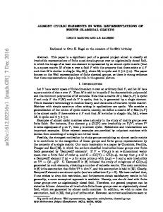
Our method is to analyze a geometric configuration of circles on the boundary of . This is appropriate because it is by the existence of such circles that -Schottky groups and non-separating disjoint circle groups are defined. We find geometric configurations that have extra tangencies, that is, those one might expect to be configurations that give a boundary group. However, we prove that not all of these potential boundary groups are actual boundary groups: they have neighborhoods where the tangencies can be pulled apart. For example, given the fundamental domain (Figure 1) for , we may remove the tangency by replacing the circle and its image with the Jordan curve and its image shown in Figure 2. The Jordan curve is chosen to agree with the circle except near the point of tangency. Alternatively, one can replace with a nearby circle ¼ and its image circle ¼ . We are interested in this second situation. It is shown in Figure 3. As the number of sides and tangencies increases, the analysis becomes more subtle. Our main tool is simply to relate the geometric configurations to algebraic parameters and to use some analytic tools to find boundaries.

7


¿

¿

¾

¾

½ -¾ -½ -½

½

¾

¿

-¾

3.1

-¾ -½ -½

½ ¾

¿

-¾

-¿ Figure 1: Tangent sides

3

½

¿ ¾

¼

½ -¾ -½ -½

½

¼

¾

¿

-¾

-¿ Figure 2: Jordan curves

-¿ Figure 3: New circles

Preliminaries Möbius Transformations

A non-singular matrix

with complex entries acts on , the sphere at infinity, as a fractional linear transformation. We often do not distinguish notationally between a matrix and the mapping it induces on . Since a matrix and its negative determine the same action, all fractional linear transformations can be considered as elements of . Unless otherwise required by the situation, we assume pull backs of elements to have positive trace. In particular, for a two generator group, once the signs of the trace of the (pull backs) of the generators are chosen, the signs of the races of all other elements of the group are determined. Elements of , or equivalently , are classified by the square of their traces. We use the term loxodromic to include both purely hyperbolic and strictly loxodromic transformations. We let denote ; the trace of is , where . A parabolic element has a unique fixed point on the boundary of which will often be referred to as a cusp. 3.2 Kleinian groups If a subgroup of is discrete, it is called a Kleinian group. We term an ordinary point if it has a neighborhood ! such that ! ! for at most finitely many . The set of ordinary points is denoted by and is also known as the regular set or the set of discontinuity. A Kleinian group is said to be of the second kind if is non-empty. By definition, the limit set of is the complement in of the ordinary set and is denoted by . If is a non-elementary Kleinian group, then is the set of

8


accumulation points of the orbit of any point in under . If is discrete, we can form the quotient . Provided contains no elements of finite order (that is, no elliptic elements), it is a three-manifold; otherwise it is an orbifold. The conformal boundary of is determined by the action of on the sphere at infinity and is the quotient of under the action of . It is a consequence of a theorem of Ahlfors [1] that if is a finitely generated Kleinian group of the second kind, then is an analytically finite Riemann surface. That means that is a Riemann surface of finite type or a disjoint union of a finite number of Riemann surfaces of finite type where every boundary component has a neighborhood conformally equivalent to a punctured disc. Even if elliptics are present, the quotient will be a Riemann surface (see Theorem 6.2.1 of [2]). Further, it is shown in [21] that a finitely generated free Kleinian group is geometrically finite if and only if every parabolic fixed point is doubly cusped, that is, the punctured discs occur in pairs.

Figure 4: Some pinchable curves on a surface of genus two. The surface is the quotient of a rank two Schottky group. The curves and are the images of the sides of the Schottky domain. and are curves that can be pinched to form a noded surface of genus two with two double cusps. If is pinched, a pair of once-punctured tori is obtained. 3.3 Noded surfaces and pinching point with a neighborhood isomorphic to

A node on a Riemann surface is a

" "

([3, 4]). In particular, a doubly cusped parabolic fixed point corresponds to a node on . If is a Riemann surface with nodes, then nodes is a disjoint union of Riemann surfaces, called the parts of . We require that every part be a Riemann


9

surface of type # , where # is the genus and the number of punctures and # . The genus of a noded surface is the genus obtained by thickening # . If the noded surface has genus the nodes, that is, two, the possibilities for number of parts, the genus of the parts and the number of nodes are easily enumerated. Intuitively, a noded surface can be viewed as obtained from the original surface by pinching along certain curves. To make this notion more precise, recall that if $ is any free group, then an element % in $ is primitive if there is a minimal generating set for $ containing it (see [18]). An element of a group is primary if it is not a power of any other element of the group. Definition 3.1. A surface $ $ (respectively the group $ ) is obtained from $ $ (respectively from $ ) by pinching % if there is an isomorphism of $ onto $ which sends a non-parabolic primary element % to a parabolic. A result of Yamamoto ([31]), stated for two generator groups, says the following. Let $ be a Schottky group of rank two with loxodromic generators . $ $ defined Consider simple disjoint geodesics , & , on by the words % % , where each % is primary in $ and for ' the cyclic subgroups generated by % and % are not conjugate in $ . There is then a Schottky type group $ and an isomorphism ( $ $ where ( % ( % and their powers and conjugates are exactly the parabolic elements of $ . Such a set of geodesics is known as a set of pinchable geodesics [10]; we also call the words % % pinchable. We extend this to groups that have parabolic generators. A group È generated by two parabolics comes from a group , with loxodromic generators, by pinching along some curves, say % and % . If is any group that comes from È by further pinching along % , then can be obtained from by pinching along % % and %¼ where the curve % ¼ is sent to % under the isomorphism of onto È . A pinchable word may or may not be primitive. For example, a noded surface with two parts, one a punctured torus and the other a thrice punctured sphere, does not correspond to a group with two parabolic generators. That is, it does not arise from pinching along two primitive curves. Since È is generated by two parabolics, the surface È È represents a sphere with four punctures. Additional pinching along % will yield two thrice

10


punctured spheres when % is primitive and two once punctured tori when % is not primitive.

4

Two parabolic generator groups

From now on, we restrict our attention to non-elementary groups that can be generated by two parabolics. Such groups are determined up to conjugacy by a single complex parameter. 4.0.1 The Lyndon–Ullman parameter: . If is a marked group with two parabolic generators, and , then up to conjugation,

and

for some )

, where assume that , so that is non-elementary.

. We

This normalization was used by Lyndon and Ullman [17], who found various regions with free as shown in Figure 5.

Figure 5: The Lyndon-Ullman Free Region(s) in . We note for future reference that since

(1) (2) (3)

and

and ,

Jørgensen’s inequality [11] tells us that is not discrete if " . We also note that is a conjugacy invariant of the group, .

11


4.1

The Riley Slice.

Riley [30] studied

%

*

, +

which is conjugate to when + . Now is always either a 4-punctured sphere with punctures identified in pairs or a pair of triply punctured spheres (see Section 3.3 or [27]). Using sequences of words with real traces, Keen and Series [16] explained the fractal like boundary of

is a 4-punctured sphere

which they term the Riley slice of Schottky space. It is shown in Figure 6, due to D. Wright.

Figure 6: The Riley Slice: Courtesy of David Wright

4.2 Spaces of groups. We now describe various spaces of groups. For the general cases, see Marden [21], Jørgensen, Marden and Maskit [14], or Gilman [9]. For the groups generated by two parabolics that we consider, the situation is greatly simplified, since the spaces can be described as subsets of . We regard as an element of a space when is.

12


Definition 4.1.

, -space

Marked two parabolic classical generators

is Classical -Schottky

Marked two parabolic classical -Schottky space: Two parabolic generators

is -Schottky

Two-parabolic classical -Schottky space

is nsdc

Two-parabolic -Schottky space

is marked Classical -Schottky

-Schottky space: Loxodromic - parabolic

is marked Classical -Schottky

Non-classical two-parabolic -Schottky space

.

Hence, 4.3

is non-Classical -Schottky

Summary of main results

We prove (Theorem 6.7) that

and in Sections 5 and 6 show that

The regions are shown in Figure 7. Our main results, Corollary 5.13 and Theorem 6.18, can now be summarized. Theorem 4.2. Assume that is generated by two parabolic elements and is parameterized by the complex number . Then

- ; - .


13

NSDC

NSDC

Classical

-Schottky

-

-

- -

-

- Figure 7: Superimposed Boundary Parabolas. Each point corresponds to a two-generator group. The darkest region shows a one parameter family of nonclassical -Schottky groups. The line-shaded subset of the classical -Schottky groups comprises the non-separating disjoint circle groups (NSDC groups). The unshaded region consists of additional non-classical -Schottky groups together with degenerate groups, isolated discrete groups and non-discrete groups. Points inside the Jørgensen circle ( " ) are non-discrete groups.

14


5

Non-separating disjoint circle groups: NSDC Groups

Heuristically, we can think of the space of non-separating disjoint circle groups as the set of ordered six-tuples in such that ¼ ¼ ¼ is the ortho-end of an nsdc-group. The boundary components of this space will be lower dimensional faces. In fact, they will be slices of nsdc space which correspond to certain limiting configurations of three circles that arise with one or more points coinciding and other extra tangencies among the three circles. Interior to the space, one can move the six points slightly and still obtain a group of nsdc type, that is, a discrete group. The boundary configurations of these slices are more rigid. If one moves a point on the boundary slightly, one sometimes obtains an nsdc group and at other times not. In what follows, instead of working with the parameters for , we work with the six-tuple . ¼ ¼ ¼ . At the end, we write down the matrices for and in terms of the six-tuple of complex numbers. Our final conditions are given in terms of the traces of , and . Since the answers are given in terms of traces, these are in fact conditions on the parameters for . 5.1 Generators for marked nsdc groups We want to relate the space of two-generator nsdc groups to the space of marked nsdc groups. We need to sort out the effect that a change of generators has on the non-separating disjoint circles. It is not difficult to prove the following Lemma 5.1. For a non-abelian two-generator subgroup of following are equivalent:

is marked nsdc; is marked nsdc; is marked nsdc; is marked nsdc;

is marked nsdc; is marked nsdc; is marked nsdc.

(1)

(5)

(2)

(6)

(3) (4)

(7)

, the

This implies Lemma 5.2. For a non-abelian two-generator subgroup of following are equivalent:

, the

15


(1)

is marked nsdc;

(3) nsdc;

(2)

is marked nsdc;

(4) nsdc.

Lemma 5.3. If loxodromic.

is marked

is marked

is marked nsdc with parabolic, then is

Proof. Consider and . If , and have the nsdc property, then . Hence and are strictly disjoint, and maps the exterior of the first circle to the interior of the second; thus is loxodromic. As a consequence of the above, we have Theorem 5.4. If and are parabolic, then disjoint circle group if and only if either or 5.2 Geometry and algebra two fixing / and 0 , we have Lemma 5.5. If /

0, /

is a non-separating is marked nsdc.

By noting that the half-turn is of order

, and 0 , then

/0

/ 0 /0 / 0

Our goal continues to be to relate the algebra and the geometry of the configuration. Since one can obtain the entries of the matrices from the six-tuple and vice-versa, conditions on the six-tuple translate into conditions on the matrices. In particular, the imposition of certain geometric configurations on the six points translate into discreteness conditions. Corresponding to a marked group with two parabolic generators, we analyze the boundary of the slice of NSDC space when two pairs of points coalesce. In ¼ ¼ ¼ , we assume that ¼ and ¼ and term it the six-tuple . four-point. Clearly, if . is four-point NSDC, then is tangent to at ¼ and to at ¼ . Such a six-tuple together with the circles , and is termed a four point configuration. Our aim is to give criteria as to when a four point configuration is indeed nsdc. We call a point NSDC if the corresponding configuration has the nsdc property. A four point configuration with maximal tangencies between circles is a potential

16


boundary configuration. In such a configuration, each circle is tangent to the other two. However, we shall see that not all configurations with maximal tangencies correspond to boundary points: some configurations can be pulled apart. Definition 5.6. A four point configuration corresponding to a six-tuple . is called extreme if the configuration is nsdc but in any deleted neighborhood of . , there exists a four-point . which is not nsdc and . ¼ which is nsdc. 5.3 Pulling Circles Apart We want to understand the family of circles passing through two given points in . The isometric circle of ¼ has center at ¼ and radius ¼ (as long as neither end is at infinity). Any other circle passing through and ¼ has its center on the perpendicular bisector of and ¼ . ¼ ¼ for some real number . The center Thus its center is at has been pulled back units from the midpoint of the segment connecting and ¼ along its perpendicular bisector. We let 1 denote the angle that the radius connecting to or ¼ makes with the Euclidean segment connecting and ¼ and call 1 the pull-back angle of the circle (see Figure 9).

¼

¼

Pulled back circle

¼

Isometric circle

Figure 8: Isometric and pulled back circles If we have two pairs of points,it is not difficult to analyze fully the family of pairs of circles through them; virtually all configurations of circle pairs are possible. In general, the situation is more complicated.


¼

Isometric circle

17

Pulled back

1

circle

1

Figure 9: Pull back angle 1 Tangent Configurations Conjugate so that , ¼ and ¼ ¼ . This is permissible as long as our final answers involve conjugacy invariants such as trace. The first step is to find three tangent circles, and the second step is to see which configurations of tangent circles are extreme. We want to find circles , and with and tangent at ; and tangent at ; and and tangent at some point, call it . (See Figure 10.) 5.4

Figure 10: 1 - circle configuration

18


The first observation is that if and are tangent at , then their pull back angles must be the same but with opposite signs; thus, for this normalization, their radii are equal. Proposition 5.7. (1) Let and be pull-back circles with common pullback angle 1. For each angle 1, 2 " 1 " 2, there is a unique D-circle called the 1-circle which is tangent to at and tangent to .

2 and 1 , parametrically the 1-circle is given by 1 1 31 and 1 , 1 31 : 1 1 1

1 1 1 1

(2) When 1

(3) When 1 when 1

1

1 1

1 1

, the circle is: and 2, the circle is: .

1

¼ Proof. Let the six points be , ¼ , ¼ and . Let be the line through with slope 1 and be the line through and . The cases for 1 and 1 2 are clear. We assume the existence of a 1-circle for when and both have pullback angles 1 and find formulas for its center and radius which turn out to be . Let be the independent of . We continue to refer to Figure 10, where by perpendicular bisector of the segment connecting and . Replacing ¼ on as necessary, we may assume that is not parallel to . another point Let , be the point of intersection of and . Then , is the center of a circle passing through and , and the circle has the prescribed tangencies. We call this circle the 1-circle. Note that the pull-back angle 1 is thus the same as the pull-back angle 1 2. We show that and , are functions of 1 and write the coordinates of the center as , 1 , 1. Let denote the center of the circle and that of . The slope of the line passing through , and is

(1) , (2) (3)

1.

1. 1.


is . For , its perpendicular bisector passes through , and and has slope . This yields

, . 3 Dist , 3 , where Dist[ , ] denotes Dist , 3

(4) The slope of the line segment connecting

(5) (6)

19

¼

and

the distance and 3 3 and 3 are the radii of the circles, , . .

1, Dist , = Dist , . , 1 , 1 , whence , 1. Conclude from , 1 and , 1 that ¾ 1 1 1, and ¾ , , 1 1.

Writing 3 3 , 3 31 , , we have 31 , 1,

(7) Since 3 (8) (9)

(10) (11)

3

(12)

so that a point on the 1-circle has coordinates given by (13) 5.5

1 1 3 , 3

Extreme four point configurations

is said to be Definition 5.8. A configuration of three tangent circles in extreme at if the three circles , and are all tangent (so that is an NSDC point) and if every neighborhood of contains points which are , and points which are not , . Such extreme configurations cannot be pulled apart. We find potentially extreme configurations by looking at configurations with maximal tangencies and identify extreme points by looking at the Jacobian of the mapping: 1 . Proposition 5.9. The points in where the Jacobian is zero are the extreme boundary points; there is one such point for each 1. All other points either have a totally NSDC neighborhood or a totally non-NSDC neighborhood. The Jacobian is non-zero except at the point where (4)

1 1

and

1 1 1

20


NSDC

-

-

- - Figure 11: The NSDC teardrop. The teardrop represents the plot of the critical points . It is the same as the envelope of the family of 1-circles. In particular, all other points on a given 1-circle have a totally NSDC neighborhood. Points in the complex plane that lie exterior to the teardrop are of non-separating disjoint circle type. Proof. Compute partial derivatives. (1)

3 ,

3 and

, 3 ,

3 .

Computing the Jacobian and setting it equal to zero yields (2) 33 3 3,

,, , Using the facts that 33 , 3, simplify the Jacobian to obtain that the Jacobian is if and only if , .

(3)

.

3

and

(4) Compute these partials to conclude that the critical points of the Jacobian are precisely those points that satisfy: 1 Namely writing, 1 1 Since ,

,

1 1,we have 1 1 , 1 1, , 1. Thus

1 1 1 1 1 1

21


(5) Combine the fact that the distance from to , is 3 with 1 to obtain the coordinates for extreme points (equation 4). (6) If are given by the formula (4), calculate that so that is extreme.

1

It is straightforward to show that for each pair 1 , the point 1 1 or the six-tuple corresponds to an NSDC group where the three circles are tangent. For each 1, the points with exterior to the 1-circle are NSDC. 5.6

Matrix Equivalents

By Lemma 5.5,

and hence

4

and

5

5

54 and 5

As before, denotes the trace of the matrix and 6 denotes the multiplicative commutator of two matrices so, that 4 . We have shown Proposition 5.10. If 5 , 5 , and 5 , where lies exterior to the NSDC teardrop, then is discrete. If 5 , 5 , and 5 , where lies exterior to the NSDC teardrop, then is discrete.

22


This motivates the following re-normalization: The map sends the six-tuple to the six-tuple , where . When the parameter is replaced by , the teardrop is transformed into a parabola. 5.7 that

Extreme four point configurations via

½

and hence

and

½ ½

We note

Motivated by the above, we term the marked group of NSDC type if the six-tuple is NSDC and of NSDC type if the six-tuple is NSDC. By Theorem 5.4, is NSDC if and only if the marked group is either NSDC or NSDC . We write ) , as in Section 4. The four point configuration for involves a circle through

and together with a line tangent to at and a line through . may be parameterized by specifying the angle 7 between the -axis and the radial vector through , measured in the anti-clockwise direction. Thus 2 " 7 " 2. 7. Once is specified, and are The radius of is then 37 determined. We let 7 be the signed distance between and , the positive direction being the radial vector from to the center of . The condition that the configuration be an nsdc configuration for this normalization is that and be sufficiently far apart to contain and that actually lie between these two lines. The following is then the criterion we are seeking Lemma 5.11. , and form an NSDC configuration for

7 37 8 7 7 Proof. The condition 7 37 guarantees that and are suffi7 ensures that lies between and ciently far apart to contain , and

. The equivalent condition follows on noting that

7

) and 37

7

23


NSDC

NSDC

-

-

- -

-

- Figure 12: Normalization through

Figure 13: NSDC

Boundary Parabolas -

Finally, we can identify when is nsdc. Theorem 5.12.

is NSDC is NSDC

8 8

Proof. By Lemma 5.11, is NSDC

8 8 7 Maximizing the left hand side as a function of 7 gives the desired result; the maximum occurs when 7 8. Points on the boundary of -space correspond to groups with maximal tangencies that are extreme. We have shown

24


Corollary 5.13.

is NSDC

8

The boundary curve 8 gives the boundary of NSDC space in the polar coordinates 8 , and this boundary curve is the piecewise-parabola whose Euclidean coordinates satisfy , as shown in Figure 13. Finally, we put Theorem 5.12 into a conjugacy invariant form.

with 5

Theorem 5.14. Assume that NSDC if and only if

5

.

Then is

5

5 3)5 Proof. The result follows by recalling that

Since an nsdc-group is discrete, we have the following discreteness criteria. Corollary 5.15. Assume that

5

6

with 5 5 . Then

3)5

is discrete.

Ì -Schottky Groups

In what follows, we continue the goal of relating the geometry of a configuration to its algebra. One can view our results as describing precisely when requiring tangencies forces a group to be a boundary group of -Schottky space and when tangencies can be pulled apart so that the group is an interior group of -Schottky space. Section 6.2 develops the main geometric insights. Preliminary to the geometric analysis we describe the effects of marking generators. 6.1 Change of generators In this subsection, we prove a series of lemmas, the first of which is an easy observation. These lead up to the proof of Theorem 6.7 about the relation between classical -Schottky groups and marked classical -Schottky groups for groups generated by two-parabolics. Lemma 6.1. For a subgroup of

,the following are equivalent:

(1)

is marked classical

-Schottky;

(2)

is marked classical

-Schottky;


(3)

is marked classical

25

-Schottky.

We say that a fixed point of a parabolic transformation is represented on the boundary of a -Schottky domain if there is an element of the group that maps the parabolic fixed point to a point on the boundary of the domain. We prove the following refinement of a well-known result. Lemma 6.2. If is a classical -Schottky group containing a parabolic and $ is a classical -Schottky domain for , then the fixed point of is represented on the boundary of $ and two sides of $ are tangent at that point. Proof. Normalize so that fixes infinity and assume that infinity is not represented on the boundary of $ . Since is a fixed point of , is not an interior point of $ . There is then a boundary circle separating infinity from the other bounding circles. Let ¼ be the bounding circle that is paired to this and the pairing. Specifically, choose to send the exterior of ¼ to the interior of . We consider the image of $ paired to this circle, that is, $ . If is on the boundary of $ , we are done. Otherwise, $ is again a -Schottky domain for with in its exterior. Repeat this process. Since is a limit point, these nested images of $ accumulate at . However, contains the translation , so at some stage the image of $ will overlap itself. For the second part, (re)-normalize so that infinity is on the boundary and note that if only one bounding circle passes through infinity, then there would be an element which is not the identity with $ $ . If $ is a classical -Schottky domain for a group , then for any , either $ $ or $ $ . We say that $ and $ are tangent if there are circles and bounding $ with and tangent.

Lemma 6.3. Let $ be a classical -Schottky domain and a side pairing transformation. If $ and $ are tangent at 9 for some , with , , then fixes 9 . Proof. Since $ is a classical -Schottky domain, there are circles and ¼ on - $ with ¼ , where maps the exterior of to the interior of ¼ . If 9 lies interior to $ , then 9 is interior to ¼ , but $ and $ are disjoint. Thus we must have 9 ¼ . Since , , it follows that all $ are tangent at 9 for all integers . The orbit of a circle through 9 accumulates at a fixed point of

, so 9 must be such a fixed point. Lemma 6.4. Suppose is marked classical -Schottky. Then

and are loxodromic for , .

26


Proof. Let $ be a classical -Schottky domain for the marked group with pairing sides and ¼ . Then maps the exterior of to the interior of

, so the region bounded by these two circles is itself a -Schottky domain for the cyclic group generated by . Therefore, if is parabolic, the two circles and must be tangent at a point 9 . Thus $ and $ are tangent at 9 . But then by Lemma 6.3, 9 is fixed by . Therefore, both and the sides of $ paired by are tangent at 9 . However, since there are no elliptic elements in -Schottky groups, such a configuration is impossible. Therefore, must be loxodromic. Likewise, if is parabolic, then and must be tangent at a point : . Applying Lemma 6.3 to the domain bounded by and , which is a classical -Schottky domain for the cyclic group , we see that fixes : . Hence , and are tangent at : , which cannot happen. Thus

must be loxodromic. In contrast to the purely loxodromic case, where Chuckrow [5] has shown that every Schottky group is a marked Schottky group on any set of free generators, we have Theorem 6.5. Suppose that is a marked classical -Schottky group. If can also be generated by parabolic elements and then, up to conjugacy, interchange of generators and replacing a generator by its inverse, we have either

(i)

and

or

(ii)

and

Proof. Let $ be a classical -Schottky domain for the marked group . Observe that $ can have at most six points of tangency; that is, the four circles that bound $ can have a total of at most six points of tangency. If any two circles are tangent at a point, none of the other four circles can be tangent at that point, and each circle can be tangent to at most two others. Since the fixed points of both and are represented on the boundary of $ as points of tangency by Lemma 6.2 (see Figure 17), there are words % and % with fixed points on the boundary of $ that are conjugate to and respectively. However, there may not necessarily be a single element of the group that conjugates % to and % to . Interchanging and if necessary, we may conjugate so that the fixed point of

lies on the boundary of $ and is fixed by the shortest possible word in and . Elements of the group send points of tangency of $ to points of tangency of the image of $ and parabolic fixed points to parabolic fixed points. We observe that the


27

generators and must each permute the parabolic fixed points on the boundary of $ : if identifies and and identifies and , we assume # is a parabolic fixed lying on and consider the possibilities for its images. Since if # lies on , is either tangent to , or at #; and by Lemma 6.2, is tangent at # to one of , or . Considering all possible cases of tangency points under the action of the group, we conclude that it suffices to consider the three cases in which the length of is at most three. Now if ! and ; are associated primitive elements of the free group on two generators, then the only primitive elements associated to ! are of the form ! ; ! , where / 0 and < (p.169 of [18]). We apply this to the cases where the length of is at most three. Length 1. is a word of length one in and . We may assume that and note that, up to conjugacy by a power of , we get ¦ . By Lemma 6.4, either or . The theorem follows after a re-normalization. Length 2. is a word of length two in and . We may assume that and . By Lemma 6.4, either or . If or , then up to conjugacy, has length one. If , then Lemma 6.4 shows that is loxodromic. Both cases are contrary to assumption. Length 3. is a word of length three in and . We may assume that . However, by Lemma 6.4, is then loxodromic, contrary to assumption. Lemma 6.6. If is marked classical -Schottky with and parabolic, then is marked classical -Schottky. . Proof. Normalize so that and and hence A -Schottky domain $ for is then bounded by and , where pairs sides and that meet at infinity and pairs circles and inside the domain bounded by and . By Lemma 6.2 and Theorem 6.5, 0 lies on the boundary of $ . There are the following three cases.

(1)

on , on . Since the Euclidean line separates .

(2)

(3)

and , we must have

is interior to the domain bounded by and with and tangent at . In this case, is interior to the region bounded by and , and . is on . Again, is tangent to at , and is tangent to at .

28


We have

.

In case (3), we let be a line orthogonal to the line joining the centers of and and separating the interiors and . Such a line exists, since and are and , then pairs and and at worst tangent. If pairs and . Thus is marked classical -Schottky. Theorem 6.7 is a direct consequence of Lemmas 6.1 and 6.6, together with Theorem 6.5. Theorem 6.7. If and are parabolic, then -Schottky if and only if is classical -Schottky.

is marked classical

6.2 Geometry of marked two parabolic generator -Schottky groups. In what follows, we consider a marked group with two parabolic generators, and , and parameter (Section 4) the complex number . We write with ) . Replacing by , if necessary, we may assume by Lemma 6.1 that 8 " 2 . The parameter ) that comes from the normalized generators determines certain geometric parameters which we describe below. Our goal is to determine how the geometric parameters determine and 8 , the algebraic parameters defined in Section 4. We consider pairing circles and and mapping the exterior of to the interior of and the translation pairing distinct lines to . Since and are parabolic, is tangent to at , the fixed point of , just as is tangent to at infinity, the fixed point of . The configuration , , and determines a classical -Schottky domain provided that and lie in the region bounded by and . If they do, then is discrete and a classical -Schottky group. We thus assume that lies in the region bounded by and . Definition 6.8. We call a classical -Schottky group and the corresponding classical -Schottky configuration extreme if every deleted neighborhood of the parameter contains points for which the group is not classical -Schottky and points for which it is classical -Schottky. Note that if either is not tangent to either circle or is not tangent to either circle, then the configuration is not extreme. Indeed if is sufficiently close to , one can easily find ¼ paired to ¼ by so that , lie strictly within the strip bounded by ¼ and ¼ .

29


The situation is more subtle if is tangent to and is tangent to . Clearly, extreme configurations are of this type. However, it turns out that not all such configurations are extreme. That is, generically one expects an extreme configuration to have six tangencies; but not all six tangency configurations are extreme, and a candidate for an extreme configuration may have only four tangencies.

¼

Classical

-

¼

Figure 14: -Schottky configuration: Two parabolic generators.

-

-Schottky

- Figure 15: Boundary Parabolas Classical -Schottky

6.2.1 The parameters , 7 and ( . We want to assign geometric parameters to the set of four circles. Let the two circles and be tangent at and assume that the line connecting their centers makes an angle 7 with the -axis. Let = ) and assume that the center of is / = . so that is parabolic, we Applying Lemma 8.3 to this situation with > obtain Corollary 6.9. If the center of is at = , the center of is at == = . The exterior of is mapped to the interior of if and only if = = . Observe that by Corollary 6.9, in order for the exterior of to be mapped to the interior of it is necessary that 7 2. Assume that the perpendicular to and makes an angle 7 ( with the -axis, ( 2.

30


Definition 6.10. Let and .

7 ( denote the Euclidean distance between

Definition 6.11. Let 7 ( be the distance between the parallel lines ¼ and ¼ , where ¼ is tangent to and parallel to and ¼ is tangent to , with ¼ and ¼ chosen so that and lie between ¼ and ¼ . We emphasize that the condition that we have a -Schottky configuration is thus precisely that . In what follows, we progressively describe how best to choose the geometric parameters 7 ( . Essentially, we minimize as a function of , then 7, and then ( . Lemma 6.12.

7 (

)

Proof. The result is a straightforward computation. Definition 6.13.

7.

Lemma 6.14. For fixed 7 and ( , there is a -Schottky configuration if and only if 7 ( 7 ( , where 7. When , 7 ( ( 7, this value of is a minimum, and the circles have the same radius. Proof. By Lemma 6.12,

( 7 7 7

and the result follows. Definition 6.15.

7

8 ( 8 ( 2

when when

8 ( 8(

In both cases,

7 2

Lemma 6.16. For fixed ( , there is a -Schottky configuration if and only if 7 ( 7 ( , where 7 satisfies 6.15.


31

Proof. By Lemma 6.14, there is a -Schottky configuration if and only if

)

( 7

Further,

)

( 7

if and only if

8 ( 8 ( 7 ( and the result follows by maximizing the left hand side as a function of 7.

Utilizing the above, we explicitly characterize classical -Schottky groups on two parabolic generators. Theorem 6.17.

8 " 2, is marked classical

-Schottky if and only if

8 If the above inequality holds, then a -Schottky configuration may be obtained by choosing

(

2

7

8 2

8 2

and

Further, the two choices of triples above, 2 7 and 2 7 , are the only choices of parameters ( 7 guaranteed to give a classical -Schottky configuration for every 8 8 " 2 . If 8

, then every classical -Schottky configuration can be obtained by choosing some ( , then setting 7 7 according to Definition 6.15. Proof. From the proof of Lemma 6.16, is marked classical -Schottky if and only if

8 ( (

But

8 ( (

32


8 (

and

or

or

and

and

" 8(

8 (

and

" 8(

Provided 8 , the maximum of the left hand side as a function of ( occurs precisely when ( 2. If 8 , then the left hand side is independent of ( , so any ( may be chosen.

Figure 17 illustrates the generic extreme configuration (i.e., 8 ). As a consequence, we can explicitly describe the boundary of classical Schottky space with two parabolic generators simply as a portion of a parabola (Figures 15, 7). We have ) Theorem 6.18. lies on the boundary of classical -Schottky space

and thus, eliminating 8 ,

) 8

with

. Finally, we put Theorem 6.17 into a conjugacy invariant form, Theorem 6.19. If -Schottky if and only if

with 5

5

, then is classical

5 ?@5 Proof. The result follows by recalling that

5

This translates to the following sufficient condition for discreteness. Corollary 6.20. If

with 5 5 ,

5 ?@5 implies that is discrete.

33


6.3 Generically not pinching A point in the two-parabolic -Schottky space represents a surface that has been pinched precisely when a new conjugacy class of primary parabolic elements appears. That is, boundary points come from additional pinching only when the pinched groups have a third conjugacy of primary parabolics. This third conjugacy class may or may not be primitive. A corollary of our results is that points on the boundary - of the classical -Schottky space generically do not arise from further pinching. Indeed, we show that there are only four values of for which the - correspond to additional cusps. Theorem 6.21. Let be the marked classical -Schottky group The only words that can be generated by parabolic elements and

. pinched to give an additional parabolic are, up to conjugacy, ¦ and . At most one of these can be pinched. Proof. Recall that after replacing by , if necessary, we may assume without loss of generality that ) , with 8 " 2 . Let $ be the classical -Schottky domain for , given in Theorem 6.17 by the triple ( 7 , where = and

(

2

7

8 2

=

The points of tangency of $ , not fixed by or

= =

) 7

= =

are as seen in Figure 17:

If a word % not conjugate to a power of or is parabolic, then by Lemma 6.2, its fixed point must be represented on the boundary of any classical -Schottky domain for and in particular, on $ . For this to happen, some of the points of tangency must be paired by . We consider the various possibilities (see Figure 17).

. In this case, = , so 8 and hence and = . Thus, is parabolic fixing . . In this case, =, so 8 2 and hence and = . It

follows that the four points are -equivalent and that parabolic fixing .

=

.

. In this case, we again have 8

2 and hence

is

and

34


. In this case, 8

Since the effect of replacing

2, by

and =

.

is to replace by , we have shown

Corollary 6.22. The only values of on the boundary of classical -Schottky space that arise from additional pinching are .

3

1

2 2

1 4

Figure 16: Four tangency extreme classical -Schottky configuration: Classical Domain

Figure 17: Six tangency extreme Schottky configuration: Classical Domain

Remark 6.23. Note that when , the points and are not equivalent. Indeed, is the ideal triangle group and has a classical -Schottky domain with only four points of tangency, as shown in Figure 16. In this case, the curve , shown in Figure 4, has also been pinched; and the noded surface comprises two triply punctured spheres.

Remark 6.24. When , the points , , and are all equivalent. In this case, the curve , shown in Figure 4, has also been pinched; and the noded surface again comprises two triply punctured spheres. Remark 6.25. Since any classical -Schottky possesses a six tangency domain, a two-parabolic generator M o¨ bius group is classical -Schottky exactly when, up to conjugacy, it has -Schottky domain

! " " "


7

35

Non-Classical Ì -Schottky Groups

We continue with , , and 7, 8 as before and obtain criteria for the infinitely generated group # to be classical -Schottky with equal sized circles. Since is a normal extension of #, the two groups have the same limit set and thus must be simultaneously discrete or non-discrete. However, we show that # is classical -Schottky at times when is non-classical -Schottky. Following [17], we define the region * to be the convex hull of the set consisting of the circle and the points . We prove that not being in the interior of * is a sufficient condition for to be -Schottky. An immediate consequence is that such groups are free, as was shown in [17].

¼

¼

Figure 18: An Example of a Non-Classical -Schottky Domain. For the non-classical -Schottky domain shown, ) , so we normalize via to obtain and . Thus pairs the circle ´ ¿µ ¿ ) , with the circle ¼ ) , and pairs with ¼ .

Lemma 7.1. Assume # with 8 2 is marked classical -Schottky with equal sized circles. Then # is marked classical -Schottky if and only if

36


!)

Proof. # is a marked classical and only if, for some 7, the circles

2 8 2

and or and

8 2

-Schottky group with equal sized circles if

) 7 7

for are disjoint. This holds if and only if

7

) 7 7 For a given 8 , we therefore need to find the minimum 7 for which the following

and

hold:

7 Thus

7 The lemma follows.

8 2

and

) )

when

2 8 2

when

8 2

Lemma 7.1 gives conditions as to when the infinitely generated group is “marked classical -Schottky.” We want to produce a set of Jordan curves for the two be the circles of equal radii passing through the generator group. Let and origin, with mapping the exterior of to the interior of . The inequalities assure that there is a Jordan curve 4 passing through , separating the interiors of and from those of and , and such that the curves , , 4 , and 4 bound a non-classical -Schottky domain for . Note that 4 may be tangent to one or all of , , and . This shows that the two generator group is non-classical -Schottky. An example of an explicit non-classical -Schottky domain is shown in Figure 18. In Figure 15, the set of classical -Schottky groups is shown with its bounding parabolas superimposed on the Riley Slice. One can thus view (numerically) the set of non-classical -Schottky groups. As a consequence of Lemma 7.1, we have a precise description of a subset of these shown in dark gray in Figure 7.

37


Let K be the set considered by Lyndon and Ullman in Figure 5. Namely, if is in the first quadrant it must satisfy

"

!) "

and or and

2 8 2

8 2

Theorem 7.2. If lies in the first quadrant below the -Schottky parabola and exterior to * , then is a non-classical -Schottky group. The above may be phrased as a criterion for a M o¨ bius group to be -Schottky.

with 5 5 , then is

Theorem 7.3. If

5

!5 )

2 $5

and or and

2

$5 2 5

Proof. The result follows by recalling that

8

-Schottky if

Marked groups with Loxodromic - Parabolic generators.

In order to complete the description of the marked classical -Schottky spaces, we need to describe the boundary for case (ii) of Theorem 6.5.

We define 3

and #

Hence, as un-marked groups

#

3 and note that 3

#

is marked classical -Schottky

#-

is marked classical -Schottky

. Further, the following are equivalent:

# is marked classical -Schottky #- is marked classical

Schottky.

As depicted in Figure 19, we can now describe when # is marked classical. Theorem 8.1. ?@ .

#

is marked classical

-Schottky if and only if 3)

38


Marked Classical -Schottky

-

-

- -

Figure 19: Marked Classical -Schottky Space. Depicted is the complex -plane. For in the dark gray area # is Classical -Schottky but not marked Classical -Schottky on the generators 3 and . Proof. By the above, we may assume that lies in the first quadrant. Any -Schottky domain for # is bounded by lines and together with circles and 3 , as shown in Figure 20. Since , must be tangent to at the parabolic fixed point by Lemma 6.2. Similarly, must be tangent to at . We thereby obtain from Corollary 6.9 that for some = ,

=

= =%

and

= ) A= =%

= =%

= =

is then a -Schottky domain for the marked group # precisely when both of the following conditions hold:

does not overlap , i.e., if

= =%= = =%= = =% = =%


39

Figure 20:

-=

-

-Schottky Domain: Loxodromic - Parabolic generators

and lie between and , i.e.,if

where @

@= = &' = =% and denotes the dot product.

For fixed = , the possible are shown in Figure 21. If the argument of = is fixed, then by convexity choosing = =% achieves the largest domain of possible . Observe that this choice is equivalent to requiring that and have the same radius. For fixed , # thus possesses a -Schottky domain precisely when there exists = with 3)= such that

does not overlap , i.e.,

= =

40


@=

Figure 21: - Separation

Figure 22: = - Separation

and lie between and , i.e.,

= The above pair of conditions are shown in Figure 22. precisely when It follows that # thus possesses a -Schottky domain 3) . If this holds, then = ?@ suffices. The theorem follows. 8.1

3

Technical lemmas

Lemma 8.2. Let , and be complex numbers and 3 a real number with . Then

Lemma 8.3.

The following are elementary computations.

>

>

>

3 3 3

3 3

maps the circle

/

5 to the circle 0

if and only if

> 5 / / 5> and + 5 / 5 / Further, maps the exterior of to the interior of / " 5. 0

+


41

Acknowledgment The authors wish to thank T.Jørgensen for many helpful conversations during the preparation of this work. We thank D. Wright for giving us permission to use his drawing of the Riley slice. REFERENCES [1] L. Ahlfors, Finitely generated Kleinian groups, Amer. J. Math. 86 (1964), 413–429. [2] A. Beardon, The Geometry of Discrete Groups, Springer-Verlag, New York–Berlin (1983). [3] L. Bers, On spaces of Rieman surfaces with nodes, Bull. Amer. Math. Soc. 80 (1974), 1219–1222. [4] L. Bers, Automorphic forms for Schottky spaces, Adv. in Math. 16 (1975), 183–212. [5] V. Chuckrow, On Schottky groups with applications to Kleinian groups, Ann. of Math. (2) 88 (1968), 47–61. [6] W. Fenchel, Elementary Geometry in Hyperbolic Space, de Gruyter & Co., Berlin–New York, 1989. [7] F. Gehring, J. Gilman and G. Martin, Kleinian groups with real parameters, Communications in Cont. Math. 3 (2001), 163–186. [8] J. Gilman, A Discreteness Condition for Subgroups of , Proceedings of the Bers Colloquium,( Keen and Dodziuk eds.) Contemp. Math. , AMS, Providence, RI, October 1997, pp. 261–267.

Author: Update if possible

[9] J. Gilman, A survey of two-parabolic Schottky groups, manuscript. [10] R. Hidalgo and B. Maskit, On neo-classical Schottky groups, preprint 2002. [11] T. Jørgensen, On discrete groups of Möbius transformations, Amer. J. Math. 98 (1976), 839–849. [12] T. Jørgensen, A note on subroups of , Quart. J. Math. 28 (1977),209–212. [13] T. Jørgensen, Closed geodesics on Riemann surfaces, Proc. Amer. Math. Soc. 72 (1978), 140–142. [14] T. Jørgensen, A. Marden and B. Maskit, The boundary of classical Schottky space, Duke Math. J. (1979), 441–446. [15] L. Keen, B. Maskit and C. Series, Geometric finiteness and uniqueness for groups with circle packing limit sets, J. Reine Agnew. Math. 436 (1993), 209–219. [16] L. Keen and C. Series, On the Riley Slice of Schottky Space, Proc. LMS 69 (1994), 72–90. [17] R. Lyndon and J. Ullman, Groups generated by two parabolic linear fractional transformations, Canadian J. Math. 21 (1969), 1388–1403. [18] W. Magnus, A. Karass, and D. Solitar, Combinatorial Group Theory, Dover, New York, 1976. [19] A. Marden, The Geometry of finitely generated Kleinian groups, Annals of Math. (2) 99 (1974), 383–462. [20] A. Marden, Schottky groups and circles, Contributions to Analysis, Academic Press, New York, 1974, pp. 273–278. [21] A. Marden, Geometrically finite Kleinian groups and their deformation spaces, in Discrete groups and Automorphic Functions (W. J. Harvey ed.) Academic Press, London 1977, pp. 259–293. [22] B. Maskit, A characterization of Schottky groups, J. Analyse Math. 19 (1967), 227–230. [23] B. Maskit, Parabolic elements in Kleinian groups, Annals of Math. (2) 117 (1983), 659–668. [24] B. Maskit, Kleinian Groups, Springer-Verlag, New York, 1987. [25] B. Maskit, On spaces of classical Schottky groups, Contemp. Math (Kra and Maskit eds.) 256 (2000), 227–237.

42


[26] B. Maskit, On the topology of classical Schottky space, Contemp. Math 311 (2002), 305–311. [27] B. Maskit and G. Swarup, Two parabolic generator Kleinian groups, Israel J. Math. 64 (1988), 257–266. [28] D. Mumford, C. Series and D. Wright, Indra’s Pearls, Cambridge,New York, 2002. [29] J. Ratcliffe, Foundations of Hyperbolic Geometry, Springer-Verlag, New-York, 1994. [30] R. Riley, Discrete parabolic representations of link groups, Mathematika 22 (1975), 141–150. [31] Hiro-o Yamamoto, Squeezing deformations in Schottky spaces, J. Math. Soc. Japan 31 (1979), 227–243. [32] Hiro-o Yamamoto, An example of a non-classical Schottky group, Duke Math. J. 63 (1991), 193–197. [33] R. Zarrow, Classical and non-classical Schottky groups, Duke Math. J. 42 (1975), 717–724.

Jane Gilman ??????????? ?????????, ?????????

Peter Waterman ????????? ????????? ?????????

(Received July 7, 2004 and in revised form November 19, 2005)