Classification of oximetry signals using Bayesian neural networks to ...

Classification of oximetry signals using Bayesian neural networks to assist in the detection of the obstructive sleep apnoea syndrome

JV Marcos1, R Hornero1, D Álvarez1, IT Nabney2, F del Campo3, C Zamarrón4 1

Biomedical Engineering Group, E.T.S.I. de Telecomunicación, University of Valladolid, Camino del Cementerio s/n, 47011, Valladolid, Spain 2 Neural Computingon-linearity and Complexity Research Group, School of Engineering and Applied Sciences, Aston University, Aston Triangle, B4 7ET, Birmingham, United Kingdom 3 Hospital Universitario del Río Hortega, Servicio de Neumología, c/ Dulzaina 2, 47012, Valladolid, Spain 4 Hospital Clínico Universitario, Servicio de Neumología, Travesía de la Choupana s/n, 15706, Santiago de Compostela, Spain E-mail: [email protected], [email protected], [email protected], [email protected], [email protected], [email protected] Abstract Nowadays, polysomnography (PSG) is the gold-standard to diagnose obstructive sleep apnoea syndrome (OSAS). However, it is complex, time-consuming and expensive. Nocturnal pulse oximetry, which provides oxygen saturation (SaO2) recordings, allows us to overcome these difficulties and could be an alternative to PSG. In the present study, multilayer perceptron (MLP) neural networks were applied to help in OSAS diagnosis using information from SaO2 signals. We performed time and spectral analysis of these recordings to extract 14 features related to OSAS. According to the principle used for network optimisation, wWe compared the performance of two different MLP classifiers: maximum likelihood (ML) and Bayesian (BY) MLP networks. A total of 187 subjects suspected of suffering from OSAS took part in the study. Their SaO2 signals were divided into a training set with 74 recordings and a test set with 113 recordings to develop and validate the classifiers. BY-MLP networks achieved the best performance on the test set with 85.58% accuracy (87.76% sensitivity and 82.39% specificity). These results were substantially better than those provided by ML-MLP networks, which were affected by overfitting and achieved an accuracy of 76.81% (86.42% sensitivity and 62.83% specificity). Our results suggest that the Bayesian framework is preferred to implement our MLP classifiers. The proposed BYMLP networks could be used for early OSAS detection, contributing to and thus reduce the number of required PSGs. Keywords: obstructive sleep apnoea syndrome (OSAS), nocturnal pulse oximetry, multilayer perceptron (MLP), maximum likelihood, Bayesian inference

1 Introduction Feedforward neural networks represent a powerful tool for pattern recognition tasks. Several advantages can be found onare associated with these algorithms. Firstly, neural networks can learn from the environment in which they operate without the requirement of any previous assumption (Haykin 1996, Zhang 2000). In addition, neural networks are capable of universal approximation, i.e. they can approximate any continuous mapping, provided that sufficiently many hidden units are available (Hornik 1991). Finally, neural networks are nonlinear models. Thus, they can be applied to model real-world complex relationships (Zhang 2000). The multilayer perceptron (MLP) is the most commonly studied and used feedforward neural network. It is usually used for classification purposes since MLP networks can estimate posterior probabilities (Bishop 1995, Haykin 1999): see equation (6). These neural networks have provided promising results in a wide variety of pattern recognition problems such as handwritten digit recognition, fault diagnosis, bankruptcity prediction and medical diagnosis (Zhang 2000). Traditionally, MLP networks were based on the maximum likelihood (ML) approach were applied to solve these problems. According to this principle, network weights (w (which are the parameters of the model in a statistical sense)) are determined by minimising an objective function that represents the error between the desired output and the network output. As a result, a single set of weights is obtained as optimum. In this context, more complex models are typically better able to fit the training data. However, this does not involve necessarily imply good generalisation capability (Bishop 1995). The Bayesian (BY) framework provides an alternative approach to implement MLP algorithms. Twhich accounts for the uncertainty on in the network weights is taken into account by considering a prior probability distribution function p(w) over weight space. The prior assumption is that networks with small weights are preferred: these give rise to smoother mappings and hence the network is likely to overfit. Once the training data D is observed, the posterior probability p(w|D) can be obtained (Bishop 1995). This distribution is concentrated on weight values that are more consistent with data in the training setcan be used to integrate over all possible parameters, weighted by their probability. Moreover, it can be used to evaluate the relevance of each input variable for the network predictions (Neal 1996, Nabney 2002). The aim of this study is to analyse the performance of Bayesian MLP networks to assist in the diagnosis of the obstructive sleep apnoea syndrome (OSAS). Moreover, we compared these algorithms with maximum likelihood MLP networks. Both network models were applied in OSAS detection using information from nocturnal oxygen saturation signals. Patients affected by OSAS suffer repetitive occlusion of the upper airway during sleep, leading to a complete (apnoea) or partial (hypopnoea) cessation of the airflow (Qureshi and Ballard 2003). The recurrence of these episodes has severe implications on for the health of the patient. Indeed: for example, OSAS is considered a risk factor for the development of cardiovascular diseases such as hypertension, cardiac failure, arrhythmias and atherosclerosis (Lattimore et al 2003). Additionally, excessive daytime sleepiness due to sleep fragmentation has been pointed out as a major cause of traffic and industrial accidents (George 2001). As a result, early diagnosis of OSAS is required in order to apply an effective treatment. NowadaysCurrently, nocturnal polysomnography (PSG) is the gold standard in for OSAS diagnosis (Qureshi and Ballard 2003). This test is performed in a special sleep unit and must be supervised by a trained technician. Usually, the following recordings are monitored during PSG: electroencephalogram (EEG), electrocardiogram (ECG), electromyiogram (EMG), electro-oculogram (EOG), oximetry, nasal airflow and respiratory effort. Subsequently, a medical expert must analyse these this data to provide a final diagnosis. Despite its diagnostic reliability, PSG is complex, time-consuming and expensive (Bennet and Kinnear 1999). Therefore, simplified diagnostic techniques would be of great practical interest. Arterial oxygen saturation (SaO2) recordings from nocturnal pulse oximetry represent an alternative to PSG. These could be acquired in the home of the patient, resulting in reduced complexity and cost. Pulse oximetry is widely known in pulmonary medicine (Netzer et al 2001). It provides useful information about respiratory dynamics during sleep. Subjects suffering from OSAS are usually characterised by SaO2 signals with high instability. The

Comment [n1]: Can these be quantified here?

repetition of apnoeas is reflected by frequent drops and the corresponding restorations of the saturation value due to the lack of oxygen during each apnoeic event. In contrast, control subjects tend to present a constant SaO2 value around 97% (Netzer et al 2001). Thus, oximetry data could be usefulis useful forto detecting OSAS. Different methodologies have been previously proposed to perform OSAS diagnosis from SaO2 recordings. Visual inspection represents the easiest analysis technique (Rodríguez et al 1996). However, automated analysis would allow to reduce the time required for a final diagnosis. Conventional oximetry indices were suggested for this purpose. These indices are usually provided by the oximetry equipment. They include the oxygen desaturation index over 2% (ODI2), 3% (ODI3) and 4% (ODI4), and the cumulative time spent below a given level of saturation. Typically, a saturation level of 90% (CT90) is applied (Lévy et al 1996, Roche et al 2002, Vázquez et al 2000, Netzer et al 2001, Magalang et al 2003). Recently, signal processing techniques have been also used for automated analysis of oximetry recordings through spectral and nonlinear methods (Zamarrón et al 2003, Álvarez et al 2006, Del Campo et al 2006, Álvarez et al 2007, Hornero et al 2007). MoreoverIn addition, pattern classification techniques such as neural networks have been applied for the development of diagnostic algorithms (ElSolh et al 2003, Marcos et al 2008, Polat et al 2008). In the present study, we modelled the OSAS diagnosis problem as a pattern recognition task. Subjects must be assigned to one of two possible groups: OSAS positive or negative. Several features extracted from SaO2 recordings were fed into MLP network classifiers to identify subjects with OSAS. We evaluated and compared the capability of MLP networks developed within two different frameworks: the maximum likelihood and the Bayesian approaches. 2 Subjects and signals A total of 187 SaO2 recordings from subjects suspected of suffering from OSAS were available for the study. Usually, sleep analysis was carried out from midnight to 8:00 AM in the Sleep Unit of the Hospital Clínico Universitario of Santiago de Compostela (Spain). The Review Board on Human Studies at this institution approved the protocol. Conventional PSG and nocturnal pulse oximetry were simultaneously performed on each of the subjects. Oximetry signals were recorded by means of a Criticare 504 oximeter (CSI, Waukeska, U.S.A.) at a sampling frequency of 0.2 Hz. The equipment used to perform PSG was a polygraph (Ultrasom Network, Nicolet, Madison, W.I., U.S.A.). Signals obtained in the polysomnographic study were EEG, EOG, chin EMG, airflow (three-port thermistor), ECG and measurement of chest wall movement. These recordings were analysed by an expert according to the system by Rechtschaffen and Kales to obtain a diagnosis for each subject (Rechtschaffen and Kales 1968). Apnoea was defined as a cessation of airflow for 10 seconds or longer. Hypopnoea was defined as a reduction, without complete cessation, in airflow of at least 50%, accompanied by a decrease of more than 4% in the saturation of haemoglobin. The average apnoea-hypopnoea index (AHI) was calculated for hourly periods of sleep from apnoeic/hypopnoeic episodes captured in PSG. Finally, a threshold of AHI ≥ 10 events/h was established to determine the presence of OSAS in a subject. A positive diagnosis of OSAS was confirmed in 111 subjects, i.e. 59.36% of the population under study. There were no significant differences between OSAS OSAS-positive and negative groups in age, body mass index (BMI) and recording time. On the other hand, the percentage of males was higher in the OSAS OSAS-positive group (84.68%) than in the OSAS OSASnegative (69.74%). The initial population was randomly divided into training and test sets to develop both types of neural network classifiers. The proportion of OSAS OSAS-positive and negative subjects was preserved in each of these sets. The training set (74 subjects) was used for network optimisation. The test set (113 subjects) was applied to estimate the generalisation capability of the classifiers. Table 1 summarises the demographic and clinical data for the whole population as well as for training and test sets.

Comment [n2]: What was the methodology used? Expert judgment? Comment [n3]: When ‘OSAS positive’ is used as an adjective, it should be hyphenated. I have tried to fix all of these, but may have missed a few.

Table 1. Demographic and clinical statistics of all subjects, training set and test set. Data are presented as mean standard deviation. n: number of subjects; BMI: body mass index; AHI: apnoea/hypopnoea index computed as events for hourly periods.

Age (years) Males (%) BMI (kg/m2) Recording Time (h) AHI (events/h)



All (n = 187) 57.97 12.84 78.61 29.54 5.51 8.19 0.62

All subjects OSAS Positive (n = 111) 58.30 12.88 84.68 30.45 4.92 8.17 0.75 40.07 19.64

OSAS Negative (n = 76) 57.57 12.87 69.74 28.42 6.02 8.22 0.33 2.04 2.36

All (n = 74) 58.25 12.14 75.68 29.62 5.71 8.22 0.41

Training set OSAS Positive (n = 44) 56.73 13.61 79.55 30.19 5.09 8.20 0.49 38.11 18.18

OSAS Negative (n = 30) 59.59 10.19 70.00 28.93 6.40 8.25 0.27 2.60 2.51

All (n = 113) 57.91 13.39 80.53 29.49 5.41 8.17 0.72

Test set OSAS Positive (n = 67) 59.37 12.38 88.06 30.63 4.84 8.14 0.88 41.36 20.58

OSAS Negative (n = 46) 56.03 14.54 69.57 28.07 5.80 8.20 0.37 1.67 2.21

3 Methods Pattern recognition techniques were applied to model the OSAS diagnosis problem using oxymetry data. Our methodology involved several stages: 1) feature extraction, 2) feature preprocessing and 3) pattern classification. 3.1

Feature extraction

The purpose of the feature extraction stage was to summarise the information in SaO2 recordings using a reduced set of parameters or features. Events of apnoea are accompanied by hypoxaemia, which is reflected in oximetry signals with a marked decrease in the saturation value. These recordings tend to present a different behaviour for OSAS positive and negative subjects. Therefore, they can be useful for OSAS detection. The extracted features must provide suitable measures in order to differentiate signals from both populations. We used signal processing techniques to extract features from oximetry data. Initially, conventional statistical analysis was applied. Moreover, we analysed SaO2 signals using spectral and nonlinear methods. As stated in our previous research (Zamarrón et al 2003, Álvarez et al 2006, Del Campo et al 2006, Álvarez et al 2007, Hornero et al 2007), spectral and nonlinear features from oximetry signals provided significant statistical differences between OSAS positive and negative subjects. Finally, a total of 14 features were computed from SaO2 recordings. These can be divided into two groups: time-domain and frequency-domain features. 3.1.1

Time-domain analysis of oximetry data

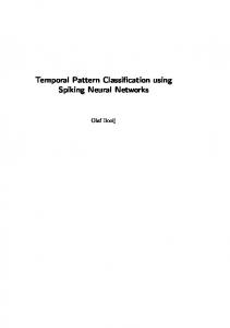
Time representation of oximetry signals reflects respiratory dynamics during sleep. Apnoea events are characterised by a decrease in the SaO2 value due to airway obstruction and reduced airflow. Therefore, signals from positive subjects are usually associated to instability. They reflect continuous drops and subsequent restorations of the saturation value because of the repetition of apnoeas. In contrast, signals from OSAS negative subjects tend to present a near

constant saturation value around 97% (Netzer et al 2001). To illustrate this, the oximetry recordings corresponding to a control subject (AHI = 0 events/h), a patient suffering from OSAS (AHI = 44 events/h) and an uncertain OSAS positive patient (AHI = 14 events/h) from our database are depicted in figure 1. In order to quantify these dynamic differences, we analysed SaO2 signals in the time domain using conventional statistics and nonlinear methods. We estimated the first four standard moments for the distribution of the variable representing the SaO2 value. The probability density function of this variable was modelled with a discrete uniform distribution. Each standard moment was estimated by averaging the values computed from signal epochs of 200 samples. The following features were extracted: 

Feature 1. First statistical moment in the time domain (SMT1). SMT1 represents the expected value for of the distribution of SaO2 samples. It is supposed to beusually lower for positive patients due to frequent drops in the saturation value.



Feature 2. Second statistical moment in the time domain (SMT2). SMT2 represents the variance for of the distribution of SaO2 samples. Positive patients are expected to provide higher values of SMT2 due to instability of their recordings.



Feature 3. Third statistical moment in the time domain (SMT3). SMT3 measures the asymmetry for of the distribution of SaO2 samples. Typically, it is negative for subjects from both populations. However, its magnitude is usually greater in positive subjects due to the higher concentration of samples with low values of saturation.



Feature 4. Fourth statistical moment in the time domain (SMT4). SMT4 evaluates the sharpness for of the distribution of SaO2 samples. It is expected to be higher in control subjects since their oximetry signals tend to be constant.

In addition, we analysed oximetry recordings with three different nonlinear methods: approximate entropy (ApEn), central tendency measure (CTM) and Lempel-Ziv complexity

Figure 1. Time representation of oximetry recordings corresponding to (a) an OSAS negative subject (AHI = 0 events/h), (b) an OSAS positive subject (AHI = 44 events/h) and (c) an uncertain OSAS positive subject (AHI = 14 events/h).

(LZC). According to our previous research, these methods can be used to evaluate properties of oximetry signals that are related to OSAS (Álvarez et al 2006, Del Campo et al 2006, Álvarez et al 2007, Hornero et al 2007). Signals were divided into epochs of 200 samples to compute these features. For each of them, the average value from all signal epochs represented the final estimate. The following nonlinear methods were applied on SaO2 signals: 

Feature 5. Approximate entropy (ApEn). ApEn estimates irregularity of time series, with high values of ApEn corresponding to irregular signals (Pincus 2001). This method requires to specifythe specification of two design parameters: a run length m and a tolerance window r. These were set to 1 and 0.25 times the standard deviation of the original sequence, respectively (Hornero et al 2007). ApEn measures the logarithmic likelihood that runs of patterns that are close (within r) for m contiguous observations remain close (within the same tolerance window width r) on subsequent incremental comparisons (Pincus 2001). Usually, high values of ApEn are associated with SaO2 signals from OSAS positive subjects. These tend to present a more irregular behaviour due to frequent changes in the saturation value (Hornero et al 2007).



Feature 6. Central tendency measure (CTM). CTM quantifies the variability of the signal (Cohen et al 1996), assigning low values to signals with a high degree of chaos. It is computed from second-order difference plots representing (st+2 – st+1) vs. (st+1 – st), where s = (s1,…, st,…, sT) is the a time series of length T. The number of points that fall inside a circular region of radius centred on the origin is obtained. Then, it is divided by the total number of points to compute CTM. In the present study, a radius = 0.25 was applied to estimate CTM from our SaO2 signals (Álvarez et al 2006). Oximetry recordings from OSAS positive patients are characterised by high variability due to the recurrence of apnoeas, which is reflected in low CTM values for these subjects (Álvarez et al 2006).



Feature 7. Lempel-Ziv complexity (LZC). LZC estimates the complexity of the signal (Lempel and Ziv 1976). Series with high complexity provide high values of LZC. It is related to the number of distinct substrings and the rate of their recurrence along a given sequence. The signal is transformed into a finite symbol sequence by comparing each sample with a fixed threshold. In this study, LZC was computed by converting SaO2 signals into 0-1 sequences. The median value of the signal samples was used as threshold (Álvarez et al 2006). The resulting sequence is scanned from left to right, increasing the complexity counter by one unit every time a new subsequence of consecutive characters is encountered (Lempel and Ziv 1976). High values of LZC are expected for SaO2 signals from OSAS positive subjects (Álvarez et al 2006).

3.1.2

Frequency-domain analysis of oximetry data

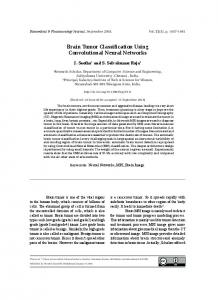
Our preceding studies concluded that spectral analysis of oximetry signals reflects significant differences between positive and negative subjects. The signal power associated with frequency components located in the band between 0.010 and 0.033 Hz is usually higher in subjects with OSAS than in normal controls (Zamarrón et al 2003). The duration of an apnoea usually ranges from 30 s to 2 min, including the awakening response after the event. The repetition of apnoeas during sleep originates phase-lagged changes in SaO2 signals with the same periodicity. Thus, the minimum and maximum frequencies for the occurrence of apnoeas would approximately correspond to the limits of that band. This behaviour is illustrated in figure 2. It depicts the power spectral density (PSD) function computed from the SaO2 recordings shown in figure 1. As it can be observed, frequent changes in the saturation value due to apnoeas lead to a higher bandwidth in SaO2 signals from positive subjects. In addition, a peak in the band between 0.010 and 0.033 Hz reflects a periodic component in the oximetry recording from the patient with severe OSAS. Different methods can be used to compute the PSD from non-stationary data such as our SaO2 signals. We applied the non-parametric Welch’s method to estimate the PSD using a

Figure 2. Power spectral density (PSD) computed from oximetry recordings corresponding to (a) an OSAS negative subject (AHI = 0 events/h), (b) an OSAS positive subject (AHI = 44 events/h) and (c) an uncertain OSAS positive subject (AHI = 14 events/h). The dashed line indicates the limits for the band between 0.010 and 0.033 Hz.

Hanning window with a length of 300 samples (50% overlapping) (Welch 1967). Initially, we analysed the statistical properties of the variable representing the frequency component of oximetry signals. The normalised PSD was used as the probability density function of this variable. The following features were computed: 

Feature 8. First statistical moment in the frequency domain (SMF1). SMF1 estimates the expected value of the variable defined by the frequency component. It is expected to beusually higher larger for OSA-S positive patients since their SaO2 signals tends to present have a higher larger bandwidth.



Feature 9. Second statistical moment in the frequency domain (SMF2). SMF2 represents the variance of the variable defined by the frequency component. Similarly, higher values of this feature are associated to patients affected by OSAS.



Feature 10. Third statistical moment in the frequency domain (SMF3). SMF3 measures the asymmetry of the variable defined by the frequency component. It is positive for both groups of subjects. High values are associated to OSAS- negative subjects since the PSD of their signals tend to be concentrated on frequencies close to zero.



Feature 11. Fourth statistical moment in the frequency domain (SMF4). SMF4 evaluates the sharpness of the distribution defined by the frequency component. It is expected to be higher for OSAS- negative subjects since the power of the signal is concentrated in low frequency components.

In addition, other three spectral features were computed from SaO2 signals. These are directly related to the analysis of the PSD in the frequency band between 0.010 and 0.033 Hz (Zamarrón et al 2003). We computed the following features:

3.2



Feature 12. Total area under the PSD (ST). ST evaluates the power of the signal under study. High values are associated to signals from positive subjects due to frequent changes and variability.



Feature 13. Area enclosed in the band of interest (SB). SB measures the signal power corresponding to frequencies in the band between 0.010 and 0.033 Hz. As indicated beforeabove, it is usually higher for OSAS- positive patients.



Feature 14. Peak amplitude of the PSD in the band of interest (PA). PA represents the most significant frequency component contained in the band between 0.010 and 0.033 Hz. It is expected to be higher in OSAS- positive patients due to periodic changes in SaO2 signals corresponding to these frequencies. Feature preprocessing

The preprocessing stage avoids possible differences between the magnitudes of the input features (Bishop 1995). Each of them was normalised to have zero mean and unit variance. The following linear transformation was applied: xin

~ xin

i

,

(1)

i

where n and i are the sample and feature indices, respectively, xin is the normalised value of x n is its corresponding raw value, feature i for sample n, ~ is the mean value of feature i and i

i

3.3

i

is its standard deviation. Classification

We used multilayer perceptron (MLP) neural network classifiers to process the normalised features. The purpose of this stage is to classify patterns from SaO2 recordings into one of two possible groups: OSAS positive or negative. MLP neural networks suitably adapt to classification tasks since they are capable of estimating posterior probabilities (Bishop 1995, Haykin 1999). Classifiers based on MLP present some advantages in comparison with other conventional techniques such as discriminant analysis. Mainly, they avoid prior assumptions about the statistical distribution of the input data (Zhang 2000). Moreover, MLP networks can establish complex nonlinear decision boundaries in the input space (Bishop 1995, Haykin 1999). For a given problem, designing neural networks requires to take some decisions about network architecture and training. In this study, input patterns must be labelled as OSAS positive or negative, which represents a two-class classification problem. A single node is required in the output layer of the network. A logistic activation function was used for this node in order to interpret network outputs as probabilities (Bishop 1995). On the other hand, we decided to evaluate MLP networks with a single hidden layer. As indicated in (Hornik 1991), networks with this architecture are capable of universal approximation. The hyperbolic tangent activation function was used for hidden nodes units since it provides faster convergence of the training algorithms (Haykin 1999). We trained our MLP networks using a coding scheme t = 1 if the input pattern belongs to class C1 (OSAS- positive group) and t = 0 if it belongs to class C0 (OSAS- negative group), with t representing the target value and Cj the membership variable. As a result, the network output can be interpreted as the probability of having OSAS given the input pattern. Therefore, the Bayes decision rule can be applied to perform pattern classification in order to minimise the probability of misclassification (Bishop 1995). It states the following:

Decide C j for x if p (C j x) max p (C j x) , j 0 ,1

where p(Cj|x) represents the posterior probability of class Cj for the input pattern x.

(2)

Training MLP networks involves to adjusting network weights from based on a finite set of data that represents the statistical properties of the problem. In this context, two different techniques can be applied: the maximum likelihood criterion and the Bayesian inference approach. In this study, we propose to compare the performance of MLP classifiers from both frameworks to assist in OSAS diagnosis using oximetry data. 3.3.1

Maximum likelihood

In classification problems, the probability of observing the target value t (represented by a 01 encoding) is modelled with a Bernoulli distribution (Bishop 1995). It is expressed as:

ptx

yt 1 y

1 t

,

(3)

where y is the network output value, i.e. the estimate for the posterior probability p(C1|x). According to this, the likelihood (L) of observing the training set is given by the following expression: N t

L

yn n 1 yn

1 tn

,

(4)

n 1

where N is the size of the training set and it has been assumed that training samples are statistically independent. The aim of the maximum likelihood approach is to adjust network weights in order to maximise L. Usually, the negative logarithm of the likelihood is considered. Then, the optimisation process is equivalent to minimise the expression resulted from that transformation. It is referred to as the cross-entropy error function (ED) and is expressed as (Bishop 1995): N

ED

t n ln yn

(1 t n ) ln( 1 yn ) .

(5)

n 1

As a result, the maximum likelihood approach allows to obtain the weight vector w that best fits the training dataThe optimal weights cannot be found directly since there is a non-linear dependence on the weights. Instead, an iterative approach is used: partial derivatives of the error function with respect to the weights can be determined analytically, and these are used in second-order non-linear optimisation algorithms. SubsequentlyAfter weight optimisation, network predictions for new input patterns are computed as: H

y

f ( x, w )

gl

I

who g t h 1

wih xi

bh

bo

,

(6)

i 1

where I is the number of features in the input vector, H is the number of hidden neuronsunits, who is the weight connecting hidden neuron unit h with output neuron unit o, bo is the bias associated to output neuron o, wih is the weight connecting the feature i of the input pattern with hidden neuron unit h, bh is the bias associated to hidden neuron unit h, gt(·) is the activation function for neurons units in the hidden layer and gl(·) is the activation function for the output layer neuronunit. 3.3.2

Bayesian inference

The Bayesian approach suggests to models the posterior probability density function of the weight vector rather than determining an optimum set of network weights (Bishop 1995, Nabney 2002). When the maximum likelihood approach is applied, dDifferent (representative) training sets representing the problem under study lead to different network weights when the maximum likelihood approach is applied. Bayesian techniques aim to consider account for this uncertainty by representing the degrees of belief in the values of the weight vector (Bishop 1995) with a probability distribution. According to the Bayes’ theorem, the posterior distribution of the weights (w) given the training set (D) is expressed as:

Formatted: Indent: First line: 0 cm

Comment [n4]: I would move this equation and the description befote equation (2).

p Dw p w , pD

p wD

(7)

where p(w) is the prior probability function over weight space, p(D|w) is the likelihood of the training data (computed using equation (4)) and p(D) is a normalisation factor known as the evidence (Nabney 2002). Once the posterior has been calculated, it can be used to infer the distribution of output values by computing the following expression: p t x, D

p t x , w p w D dw

(8)

where p(t|x,w) is the model for the distribution of the noise on the target for a given weight vector. In pattern classification problems, it is given by the expression in (3). Therefore, the probability of membership of an input pattern to the OSAS positive group is obtained as: p C1 x, D

p C1 x, w p w D dw

y x , w p w D dw

(9)

We used the evidence procedure (Mackay 1992) to implement Bayesian MLP networks. A Gaussian approximation to the posterior (Laplace approximation) is used to solve compute integrals such as those mentioned before (Nabney 2002)in equations (8) and (9). In the absence of data, the prior probability distribution is chosen in order to favour small weights. Smooth mappings are preferred since they provide better generalisation (Bishop 1995). Thus, the prior is modelled using the following zero-mean exponential Gaussian function:

pw

1 exp ZW

1 exp ZW

EW

2

w

2

,

(10)

where ZW is a normalisation factor and , is referred to as a hyperparameter, is the inverse variance of the Gaussian. It controls the distribution of other the network parameters, i.e. network weights and biases. On the other hand, the likelihood function for the training data given in (4) can be written as: N

L

t

p Dw

yn n 1 yn

1 tn

exp G D w

(11)

n 1

where G(D|w) = ED is the cross-entropy error function as in equation (5). According to the expression in (7), the Bayes’ theorem is applied to compute the posterior probability from p(w) and p(D|w). It is given by: p wD

1 exp ZS

G

EW

1 exp ZS

Sw ,

(12)

1 2 w and S(w) = G(D|w) + EW(w). 2 In practice, this distribution is approximated by a Gaussian centred on the maximum posterior weight vector (wMP): where ZS is a normalisation factor for the Gaussian, EW

p wD

1 exp Z S*

S w MP

1 wT A w 2

(13)

where ZS* is the normalisation factor for the Gaussian, Δw = w – wMP and A is the Hessian matrix of the error function S(w). The implementation of the Bayesian MLP network requires the use of a nonlinear optimisation algorithm to find wMP, which is found by minimising S(w). Additionally, the hyperparameter is periodically updated during this optimisation process. The maximum posterior value for the hyperparameter is found by maximising the likelihood p(D|α) (Bishop 1995, Nabney 2002).

The hyperparameter controls the shape of the prior distribution of weights. Complex forms of this hyperparameter can be specified. Specifically, different values of can be used to model the distribution of the weights associated to each input feature. This procedure is known as automatic relevance determination (ARD) (Neal 1996, Nabney 2002). Once the network has been trained, the importance of an input feature (xi) can be evaluated by analysing its associated hyperparameter ( i). A low value of i corresponds to a large variance prior, which allows weights of large magnitude. Thus, the feature xi is very relevant for predicting the output. Conversely, a large value of i is interpreted as low influence of the input feature on network output. As a result, feature selection is implemented in the network training process. 4 Results We computed the proposed 14 features from each SaO2 signal in our database. Table 2 summarises the mean value of each feature for the complete set of signals. Subsequently, the preprocessing stage was applied on each feature. The obtained patterns were fed into a MLP classifier. We developed MLP networks using the two optimisation frameworks described before: maximum likelihood (ML) and Bayesian inference (BY). The Netlab software was used to implement these algorithms (Nabney 2002). 4.1

Training

The training set with 74 subjects was used to develop our classification algorithms. The scaled conjugate gradient was used to optimise both types of MLP classifiers (Moller 1993). It was applied to minimise the cross-entropy error function given by ED in order to determine the optimum weight vector for networks corresponding to the ML criterion. In the BY framework, the optimisation algorithm was used to find the most probable set of weights by minimising the error function S(w); this is alternated with re-estimation of hyperparameters using the evidence framework (Mackay 1992).

Different network architectures of both types were evaluated by varying the number of hidden nodes from 2 to 20. The generalisation performance of each network configuration was measured with sensitivity, specificity and accuracy. Additionally, we used receiver operating characteristics (ROC) analysis. The area under the ROC curve (AUROC) was computed as a measure of classification ability (Hanley and McNeil 1982). Given the random nature of network initialisation, the performance measures were averaged for a total of 10 runs, i.e. a total of 10 different networks were trained for each configuration. Table 3 summarises the results achieved on the training set for both types of MLP networks. As it can be observed, ML-MLP networks can correctly classify all the samples in the training set. This is achieved for network configurations with more than 4 nodes in the hidden layer. In contrast, BY-MLP networks provided lower classification ability on the training data, reaching an accuracy value around 90% and an AUROC close to 0.95.

Table 2. Time and spectral features extracted from nocturnal oximetry recordings for all subjects under study. Data are presented as mean standard deviation. n: number of subjects; SMT1: first statistical moment in the time domain; SMT2: second statistical moment in the time domain; SMT3: third statistical moment in the time domain; SMT4: fourth statistical moment in the time domain; ApEn: approximate entropy; CTM: central tendency measure; LZC: Lempel-Ziv complexity; SMF1: first statistical moment in the frequency domain; SMF2: second statistical moment in the frequency domain; SMF3: third statistical moment in the frequency domain; SMF4: fourth statistical moment in the frequency domain; ST: total area under the power spectral density; SB: area enclosed in the band of interest; PA: peak amplitude of the power spectral density in the band of interest.

All (n = 187) SMT1 SMT2 SMT3 SMT4 ApEn CTM LZC

93.36 2.29 -0.50 4.92 0.80 0.47 0.49

5.29 2.02 0.50 2.16 0.38 0.28 0.18

All (n = 187) SMF1 SMF2 SMF3 SMF4 ST SB PA

0.0104 0.0050 0.0135 0.0031 2.85 1.56 17.03 23.41 15.21 25.75 5.88 11.51 840.75 1841.80

TIME FEATURES OSAS Positive (n = 111) 91.78 5.37 3.18 2.08 -0.60 0.46 4.25 1.64 1.03 0.28 0.30 0.20 0.60 0.13 SPECTRAL FEATURES OSAS Positive (n = 111) 0.0121 0.0139 2.27 12.11 23.31 9.51 1363.05

0.0051 0.0031 1.08 9.71 29.54 13.78 2239.52

OSAS Negative (n = 76) 95.67 0.98 -0.35 5.89 0.47 0.71 0.34

4.26 0.93 0.54 2.44 0.25 0.18 0.14

OSAS Negative (n = 76) 0.0079 0.0037 0.0130 0.0031 3.69 1.76 24.22 33.64 3.37 11.22 0.59 1.53 77.93 251.64

Table 3. Classification results achieved by maximum likelihood and Bayesian MLP classifiers on the training set. Se: sensitivity; Sp: specificity; Ac: accuracy; AUROC: area under the ROC curve. Maximum likelihood Hidden nodesunits 2 4 6 8 10 12 14 16 18 20

4.2

Bayesian inference

Formatted Table

Se (%)

Sp (%)

Ac (%)

AUROC

Se (%)

Sp (%)

Ac (%)

AUROC

99.77 ± 0.72 99.77 ± 0.72 100.00 ± 0.00 100.00 ± 0.00 100.00 ± 0.00 100.00 ± 0.00 100.00 ± 0.00 100.00 ± 0.00 100.00 ± 0.00 100.00 ± 0.00

90.33 ± 3.67 100.00 ± 0.00 100.00 ± 0.00 100.00 ± 0.00 100.00 ± 0.00 100.00 ± 0.00 100.00 ± 0.00 100.00 ± 0.00 100.00 ± 0.00 100.00 ± 0.00

95.95 ± 1.56 99.86 ± 0.43 100.00 ± 0.00 100.00 ± 0.00 100.00 ± 0.00 100.00 ± 0.00 100.00 ± 0.00 100.00 ± 0.00 100.00 ± 0.00 100.00 ± 0.00

0.98 ± 0.01 1.00 ± 0.00 1.00 ± 0.00 1.00 ± 0.00 1.00 ± 0.00 1.00 ± 0.00 1.00 ± 0.00 1.00 ± 0.00 1.00 ± 0.00 1.00 ± 0.00

92.50 ± 1.53 90.20 ± 2.64 90.90 ± 1.86 89.80 ± 1.20 88.90 ± 1.29 88.60 ± 1.07 88.00 ± 1.53 88.60 ± 0.00 88.90 ± 0.72 88.40 ± 0.72

86.70 ± 0.00 87.00 ± 1.05 87.70 ± 2.25 89.00 ± 1.61 88.70 ± 1.72 88.00 ± 2.33 87.70 ± 1.61 88.00 ± 1.72 87.00 ± 1.05 86.70 ± 0.00

90.10 ± 0.91 88.90 ± 1.66 89.60 ± 1.28 89.50 ± 0.57 88.80 ± 1.11 88.40 ± 0.70 87.80 ± 1.27 88.40 ± 0.70 88.10 ± 0.57 87.70 ± 0.43

0.96 ± 0.00 0.95 ± 0.01 0.95 ± 0.00 0.95 ± 0.00 0.95 ± 0.00 0.95 ± 0.00 0.95 ± 0.01 0.95 ± 0.00 0.95 ± 0.00 0.95 ± 0.00

Test

The trained networks were also evaluated on previously unseen data to obtain a more reliable measure of generalisation capability. The test set with 113 subjects was used. The results achieved by ML-MLP and BY-MLP networks are summarised in table 4. As expected, the results on the test set were lower than those achieved on the training set by both types of MLP networks. However, the decrease was significantly marked for ML-MLP networks. This was not very surprising. The networks have 16H+1 parameters (where H is the number of hidden units) and hence when H>4 there are more parameters than training data samples. In addition, it was observed that there were slight differences between network configurations with a different number of hidden nodes. It which was observed for both MLMLP and BY-MLP networks. Thus, less complex algorithms such as networks with 2 hidden nodes are preferred. The ML-MLP algorithm with this configuration provided a mean accuracy of 76.81% (86.42% sensitivity and 62.83% specificity) and a mean AUROC of 0.86. The accuracy reached by BY-MLP classifiers on the test set was substantially higher. The BY-MLP network with 2 nodes in the hidden layer achieved a mean accuracy of 85.58% (87.76% sensitivity and 82.39 % specificity) and a mean AUROC of 0.90.

Formatted: Font: Italic Formatted: Font: Italic Formatted: Font: Italic

Comment [n5]: I would also include results from logistic regression as comparison.

Table 4. Classification results achieved by maximum likelihood and Bayesian MLP classifiers on the test set. Se: sensitivity; Sp: specificity; Ac: accuracy; AUROC: area under the ROC curve. Maximum likelihood Hidden nodesunits 2 4 6 8 10 12 14 16 18 20

Bayesian inference

Formatted Table

Se (%)

Sp (%)

Ac (%)

AUROC

Se (%)

Sp (%)

Ac (%)

AUROC

86.42 ± 1.79 82.39 ± 5.53 84.48 ± 5.37 84.33 ± 3.32 85.37 ± 3.57 85.97 ± 1.75 84.93 ± 2.77 84.78 ± 4.15 84.33 ± 3.39 85.67 ± 1.04

62.83 ± 3.90 67.39 ± 3.24 68.04 ± 2.91 66.74 ± 3.56 66.74 ± 2.72 65.87 ± 3.56 66.74 ± 1.79 65.87 ± 2.06 67.39 ± 3.69 64.57 ± 2.30

76.81 ± 0.91 76.28 ± 3.68 77.79 ± 3.08 77.17 ± 1.71 77.79 ± 2.45 77.79 ± 1.93 77.52 ± 1.68 77.08 ± 2.75 77.43 ± 1.78 77.08 ± 1.14

0.86 ± 0.04 0.84 ± 0.02 0.84 ± 0.03 0.81 ± 0.03 0.82 ± 0.03 0.82 ± 0.02 0.82 ± 0.01 0.81 ± 0.03 0.81 ± 0.03 0.80 ± 0.01

87.76 ± 0.63 85.07 ± 4.39 86.42 ± 0.47 86.27 ± 0.63 86.42 ± 1.10 85.82 ± 1.61 85.37 ± 1.37 85.82 ± 1.27 85.37 ± 1.54 85.37 ± 1.54

82.39 ± 2.39 84.57 ± 0.69 84.13 ± 1.05 84.78 ± 0.00 84.78 ± 0.00 84.78 ± 0.00 84.78 ± 0.00 84.78 ± 0.00 84.78 ± 0.00 85.00 ± 0.69

85.58 ± 0.84 84.87 ± 2.87 85.49 ± 0.62 85.66 ± 0.37 85.75 ± 0.65 85.40 ± 0.96 85.13 ± 0.81 85.40 ± 0.75 85.13 ± 0.91 85.22 ± 0.84

0.90 ± 0.00 0.89 ± 0.01 0.90 ± 0.01 0.90 ± 0.00 0.90 ± 0.00 0.90 ± 0.00 0.90 ± 0.00 0.90 ± 0.00 0.90 ± 0.00 0.90 ± 0.00

5 Discussion Classifiers based on Bayesian MLP networks were evaluated as an assistant tool to assist in OSAS diagnosis from nocturnal oximetry data. A total of 14 features computed from timedomain and frequency-domain analysis of SaO2 signals were used as inputs. The performance of these classifiers was compared with that achieved by common ML-MLP networks. We found that the classification ability of these algorithms was improved by BY-MLP. Our results indicate thatusing Bayesian inference represents a more effective optimisation technique to implement our MLP classifiers. It is often preferred in applications with a reduced small dataset such as that presented in this study. BY-MLP networks provided the best classification performance with an accuracy of 85.58% and an AUROC of 0.90 on the test set. These networks significantly outperformed classifiers based on ML-MLP (76.81% accuracy and 0.86 AUROC). The opposite situation was observed for data in the training set. The accuracy reached on this set by BY-MLP networks ranged from 87.70% (BY-MLP with 20 hidden nodes) to 90.10% (BY-MLP with 2 hidden nodes). For MLMLP networks, it was close or equal to 100%. The comparison of the results achieved on both sets indicates that ML-MLP networks overfitted the training data. These networks are more likely to be affected by overfitting since their inherent complexity is greater than that of BYMLP networks (Bishop 1995). For a given training set, the bias-variance trade-off requires the best compromise between a good representation of the data and network complexity in order to achieve high generalisation capability. A simple or inflexible model (large bias) can lead to underfit the data. The model may not have the ability to learn enough the underlying distribution. On the other hand, a too complex or flexible model (large variance) could capture the noise present in the training data, leading to overfitting. Both situations result in poor generalisation (Bishop 1995, Haykin 1999). The main advantage of BY-MLP networks is that the effect of the bias-variance dilemma is no relevantreduced. They implement regularisation by including the hyperparameter , which controls the distribution of the weights and the network complexity during training (Nabney 2002). Many real applications such as the proposed OSAS diagnosis problem present a training set with a limited size. Thus, regularisation techniques are required to develop effective neural network algorithms. In our preceding work, an MLP network with nonlinear features from oximetry data was developed to help in OSAS diagnosis (Marcos et al 2008). It provided an accuracy of 85.5% and an AUROC of 0.90 on a test set with 83 subjects using weight decay regularisation. These results were similar to those obtained with BY-MLP networks developed in this study. However, weight decay requires the user to adjust an additional regularisation parameter, which controls the trade-off between reducing training error and favouring small weight values. A high large number of experimental runs are needed to optimise this parameter. Therefore, the Bayesian approach represents a more efficient regularisation technique since the hyperparameter is automatically updated in the training process. Moreover, it allows us to specify complex priors to implement automatic relevance determination. This procedure provides a means to perform feature selection in the network training algorithm (Nabney 2002). From our experiments, we found that ApEn, LZC, SMT1 and SMT4 were determined as the most relevant features to classify SaO2 recordings as OSAS- positive or negative. This result suggests that time-domain features from oximetry data provided the most relevant information to detect OSAS. Other methodologies to analyse oximetry signals for OSAS diagnosis were have been previously proposed to analyse oximetry signals for OSAS diagnosis. Visual inspection of these recordings provided a sensitivity of 91% and a specificity of 69% (Rodríguez et al 1996). However, this is a time-consuming technique and the interpretation of the signals may differ from one expert to another. Conventional oximetry indices were proposed for automated analysis of SaO2 recordings. Most of the commercial oximeters can provide ODI2, ODI3, ODI4 and the cumulative time spent below 90% of saturation. The diagnostic capability of these indices has been evaluated in other studies. The reported results varied among different researchers: the sensitivity ranged from 31% to 98% and the specificity from 41% to 100% (Netzer et al 2001). Vázquez et al (2000) reported 98% sensitivity and 88% specificity by

Comment [n6]: i.e. time-domain features were better than frequency-domain features Comment [n7]: Include a table of final alpha values for each feature. Ideally, it might also be good to train some models on a reduced set of inputs to see if this improves performance. Comment [n8]: It would be very helpful to include Accuracy (and where posible AUROC) values in this paragraph. Perhaps a summary table of the algorithm results would also help.

means of ODI4 when a threshold of 15 events/h was applied to define OSAS. It represents the highest diagnostic accuracy reported by these indices. However, a definition of arousal different to the criteria proposed by the Atlas Task Force was applied (The Atlas Task Force 1992). Lévy et al (1996) proposed an additional index (Δ index) from oximetry signals to detect OSAS. It is a measure of the variability of the SaO2 recordings. This parameter achieved 98% sensitivity and 46% specificity using a threshold of 15 events/h on the AHI to determine the presence of OSAS. Magalang et al (2003) achieved similar results using the Δ index, with a sensitivity of 91% and a specificity of 59%. These results were improved by using the Δ index together with the other conventional indices, which yielded a sensitivity of 90% and a specificity of 70%. Finally, Roche et al (2002) suggested to combine information from oximetry data with clinical features using logistic regression. This model achieved an accuracy of 62.1%. The presented algorithms improved the classification accuracy reported in the cited studies. Moreover, we used our database of SaO2 recordings to compare the diagnostic capability of our networks and conventional oximetry indices. In order to do this, we computed the classification results of these indices on our signal database. For each index, the threshold (l) that provided the highest accuracy on the training set was selected. Subsequently, it was applied on signals in the test set to compute sensitivity, specificity and accuracy values. In addition, we computed the AUROC from data in the test set. The obtained results are summarised in table 5. The best diagnostic performance was provided by ODI2 and ODI3, which achieved a sensitivity of 76.12%, a specificity of 93.48% and an accuracy of 83.19%. In addition, CT90 provided the best AUROC value with 0.77. As it can be observed, the BY-MLP classifiers clearly outperformed conventional oximetry indexes. The proposed algorithms represent a more effective technique for automated OSAS diagnosis from SaO2 data. Some limitations can be found in our methodology. A larger population would be desirable to obtain a better representation of the statistical properties of our classification problem. The generalisation capability of our networks could be improved by using a larger training set. Similarly, a more accurate estimate of our classification results could be obtained through a larger test set. Moreover, our results were computed as the average value of several runs. A model selection stage is required in order to select an optimum classification algorithm from those trained in our experiments. In summary, BY-MLP classifiers have shown to be a useful tool to assist in OSAS diagnosis from oximetry data. They achieved an accuracy of 85.58% (87.76% sensitivity and 82.39% specificity) and an AUROC of 0.90. They outperformed ML-MLP networks, which provided an accuracy of 76.81% and an AUROC of 0.86. Our results suggest that Bayesian techniques are preferred for the optimisation of our MLP networks. In addition, the proposed BY-MLP algorithms improved the diagnostic capability of visual inspection of SaO2 recordings and conventional oximetry indices. Our BY-MLP networks could be used to assist medical experts for early detection of OSAS only using oximetry signals. These algorithms could be applied as an effective technique for OSAS screening, contributing to reduce the number of required PSG Table 5. Diagnostic results achieved by conventional oximetry indices. ODI2: oxygen desaturation index over 2%; ODI3: oxygen desaturation index over 3%; ODI4: oxygen desaturation index over 4%; CT90: cumulative time spent below 90% of saturation; l: threshold value determined on the training set; Se: sensitivity; Sp: specificity; Ac: accuracy; AUROC: area under the ROC curve. Index ODI2 ODI3 ODI4 CT90

l 9 8 7.6 11

Se (%) 76.12 76.12 73.13 68.66

Sp (%) 93.48 93.48 95.65 95.65

Ac (%) 83.19 83.19 82.30 79.65

AUROC 0.706 0.725 0.758 0.774

tests. Other possible future work – classification of segments of dataset so that a more refined diagnosis can be given; it might also increase performance.

Acknowledgment This work has been partially supported by Ministerio de Ciencia e Innovación and FEDER under project TEC2008-02241, and by Consejería de Sanidad de la Junta de Castilla y León under project GRS 337/A/09. References Álvarez D, Hornero R, Abásolo D, Del Campo F and Zamarrón C 2006 Nonlinear characteristics of blood oxygen saturation from nocturnal oximetry for obstructive sleep apnoea detection Physiol. Meas. 27 399-412 Álvarez D, Hornero R, García M, Del Campo F and Zamarrón C 2007 Improving diagnostic ability of blood oxygen saturation from overnight pulse oximetry in obstructive sleep apnea detection by means of central tendency measure Artif. Intell. Med. 41 13-24 Bennet JA and Kinnear WJM 1999 Sleep on the cheap: the role of overnight oximetry in the diagnosis of sleep apnoea hypopnoea syndrome Thorax 54 958-9 Bishop CM 1995 Neural networks for pattern recognition (Oxford University Press, Oxford, UK) Cohen ME, Hudson DL and Deedwania PC 1996 Applying continuous chaotic modelling to cardiac signals IEEE Eng. Med. Biol. Mag. 15 97-102 Del Campo F, Hornero R, Zamarrón C, Abásolo DE and Álvarez D 2006 Oxygen saturation regularity analysis in the diagnosis of obstructive sleep apnea Artif. Intell. Med. 37 111-8 El-Solh AA, Magalang UJ, Mador MJ, Dmochowski J, Veeramachaneni S, Saberi A, Draw AM, Lieber BB and Grant BJB 2003 The utility of neural network in the diagnosis of Cheyne-Stokes respiration J. Med. Eng. Technol. 27 54-8 George CFP 2001 Reduction in motor vehicle collisions following treatment of sleep apnoea with nasal CPAP Thorax 56 508-12 Hanley JA and McNeil BJ 1982 The meaning and use of the area under a receiving operating characteristic (ROC) curve Radiology 143 29-36 Haykin S 1996 Neural networks expand SP’s horizons IEEE Signal Process. Mag. 13 24-49 Haykin S 1999 Neural Networks: A Comprehensive Foundation (Prentice Hall, New Jersey, US) Hornero R, Álvarez D, Abásolo D, Del Campo F and Zamarrón C 2007 Utility of aproximate entropy from overnight pulse oximetry data in the diagnosis of the obstructive sleep apnea syndrome IEEE Trans. Biomed. Eng. 54 107-13 Hornik K 1991 Approximation capabilities of multilayer feedforward networks Neural Netw. 4 251-7 Lattimore JL, Celermajer DS and Wilcox I 2003 Obstructive sleep apnea and cardiovascular disease J. Am. Coll. Cardiol. 41 1429-37 Lempel A and Ziv J 1976 On the complexity of finite sequences IEEE Trans. Inf. Theory 22 7581 Lévy P, Pépin JL, Deschaux-Blanc C, Paramelle B and Brambilla C 1996 Accuracy of oximetry for detection of respiratory disturbances in sleep apnea syndrome Chest 109 395-99 Mackay DJC 1992 The evidence framework applied to classification networks Neural Computation 4 720-736 Magalang UJ, Dmochowski J, Veeramachaneni S, Draw A, Mador MJ, El-Solh A and Grant BJB 2003 Prediction of the apnea-hypopnea index from overnight pulse oximetry Chest 124 1694:701 Marcos JV, Hornero R, Álvarez D, del Campo F, Zamarrón C and López M 2008 Utility of multilayer perceptron neural network classifiers in the diagnosis of the obstructive sleep apnoea syndrome from nocturnal oximetry Comput. Meth. Programs Biomed. 92 79-89 Moller MF 1993 A scaled conjugate gradient algorithm for fast supervised learning Neural Netw. 6 525-33 Nabney IT 2002 Netlab: algorithms for pattern recognition (Springer, LondonBerlin, Germany)

Formatted: Font: Italic Formatted: Font: Bold

Neal, RM 1996 Bayesian learning for neural networks, Lecture notes in statistics 118 (Springer, New York) Netzer N, Eliasson AH, Netzer C and Kristo DA 2001 Overnight pulse oximetry for sleepdisordered breathing in adults: a review Chest 120 625-33 Pincus SM 2001 Assessing serial irregularity and its implications for health Ann. NY Acad. Sci. 954 245-67 Polat K, Yosunkaya S and Günes S 2008 Comparison of different classifier algorithms on the automated detection of obstructive sleep apnea syndrome J. Med. Syst. 32 243-50 Qureshi A and Ballard RD 2003 Obstructive sleep apnea J. Allergy Clin. Immunol. 112 643-51 Rechtschaffen A and Kales A 1968 A manual of standardized terminology, techniques and scoring system for sleep stages of human subjects (Brain Information Services, Brain Research Institute, University of California, Los Angeles, US) Roche N, Herer B, Roig C and Huchon G 2002 Prospective testing of two models based on clinical and oximetric variables for prediction of obstructive sleep apnea Chest 121 747-52 Rodríguez JM, De Lucas P, Sánchez MJ, Izquierdo JL, Peraíta R and Cubillo JM 1996 Usefulness of the visual analysis of night oximetry as a screening method in patients with suspected clinical obstructive sleep apnea syndrome Arch Bronconeumol 32 437-41 The Atlas Task Force 1992 EEG arousals: scoring rules and examples. A preliminary report from the Sleep Disorder task Force of the American Sleep Disorders Association Sleep 15 173-84 Vázquez JC, Tsai WH, Flemons WW, Masuda A, Brant R, Hajduk E, Whitelaw WA and Remmers JE 2000 Automated analysis of digital oximetry in the diagnosis of obstructive sleep apnoea Thorax 55 302-7 Welch PD 1967 The use of fast Fourier transform for the estimation of power spectra: a method based on time averaging over short, modified periodogram IEEE Trans Audio Electroacoust 15 70-3 Zamarrón C, Gude F, Barcala J, Rodríguez JR and Romero PV 2003 Utility of oxygen saturation and heart rate spectral analysis obtained from pulse oximetric recordings in the diagnosis of sleep apnea syndrome Chest 123 1567-76 Zhang GP 2000 Neural networks for classification: a survey IEEE Trans Syst Man Cybern Part C-Appl Rev 30 451-62

Formatted: Font: Italic