Paper—Cloud Based WiFi Multi-Sensor Network
Cloud Based WiFi Multi-Sensor Network https://doi.org/10.3991/ijoe.v14i08.8536
Anekwong Yoddumnern, Roungsan Chaisricharoen, Thongchai Yooyativong Mae Fah Luang University, Chiangrai, Thailand.
[email protected]
Abstract—A WiFi technology was run on a smart device using three types of sensors: a temperature sensor, smoke-CO, and PIR sensor. This project sought to design a multi-sensor node. All of the sensors were connected to a microcontroller unit (MCU) with a general purpose input output (GPIO). After the connection, there were invalid multi-sensor data when the processor started up. First, the temperature sensor did not work. Second, the smoke-CO sensors read an invalid value higher than the actual. This situation was solved through sensor calibration methodology following calibration time and self-calibration with a Finite Impulse Response (FIR) filter. After the system ran for a long time, there were invalid data with values different than the truth. While the system was running, there was some noise and heat collected on the device, creating invalid values. These errors were solved by using the Full Scale Kalman Filter (FSKF) to estimate the right value. Next, the OFF-Mode was used to save power consumption by 37.24% before sending the sensor data to the Cloud. These methods helped the device run a long time and work a long life. Finally, there was a high-performance WiFi multi-sensor network. Keywords—WiFi, Multi-Sensor, FIR Filter, Calibrate, Calibration Time, SelfCalibration, FSKF, Kalman Filter, OFF-Mode, Low Power, Cloud.
1
Introduction
In general, a single sensor node is accessible because it merely works at a more comfortable usage level [2]. However, a single sensor node does not cover much work time. The function of a multi-sensor node is to detect and report events in a multiprocessing mode, especially in the pattern of a high-security system or as an accurate system. The multi-sensor node is a necessity in system projects – such as the Internet of Thing (IoT) [3] [5] [16]. The system can access and use the WiFi signals everywhere and at any time. The multi-sensor node can detect the analog signal and digital signal by co-operating to serve more and multiple projects. This project was run with four sensors on an microcontroller unit (MCU). They are set in a case study of a Home Security System (HSS): temperature sensor, humidity sensor, smoke sensor, and PIR motion sensor. The MCUs were an Arduino-UNO, NodeMCU and LinkIt Smart 7688 Duo. After the circuit had run 12 times—following the number of the MCUs, there was a problem with the sensors detecting invalid values. There was a goal of low cost and creating the ideal device following the current
iJOE ‒ Vol. 14, No. 8, 2018
35
Paper—Cloud Based WiFi Multi-Sensor Network
IT market with the trend of IoT [19]. Most of the sensors detected invalid low and high data values from the truth rather than smooth values. When the system ran for an extended time, the sensors detected invalid data values, especially the analog sensor. The multi-sensors detect all time and send the values to the Cloud storage via the WiFi module following each processing cycle. These are unnecessary and do not save power. Table 1 shows the experiment with some errors of data detection. Table 1. The MCUs detected signal value. Sensor Detection Type of MCU
Temperature sensor Startup
LoopDetecting
Arduino UNO#1
Invalid-high
Invalid at 463
Arduino UNO#2
Fail
Smoke detector
PIR movement detector
Startup
LoopDetecting
Startup
Invalid-high
Invalid lowhigh
-
-
-
Fail
-
Invalid low-high Invalid-high
LoopDetecting
Arduino UNO#3
Invalid-high
Invalid at 412,413
Arduino UNO#4
Invalid-high
Invalid at 224
Invalid-high
Invalid at 119
-
-
*ArduinoUNO #5
Fail
Invalid at 211,278
-
Invalid at 423
-
-
NodeMCU#1
Fail
Invalid at 342
-
-
Invalid lowhigh
Fail
-
NodeMCU#2
Invalid-high
-
-
-
Invalid low-high Invalid-high
Invalid-high Invalid at 74,266 Invalid-high
NodeMCU#3
Fail
Invalid at 320
Invalid-high
Invalid at 390
-
-
*NodeMCU#4
Fail
Invalid at 195
Invalid-high
Invalid at 287
Fail
-
*NodeMCU#5
Invalid-high
Invalid at 337
Invalid-high
Invalid at 124
-
-
LinkIt-Smart 7688 Duo
Invalid high
Invalid at 434
Invalid high
-
-
-
*LinkIt-Smart 7688 Duo
Invalid high
-
-
Invalid at 207
-
-
Invalid 58.33 %
Invalid 97.67 %
Invalid 83.33 %
Invalid 75.00 %
Fail 25.00 %
Fail 41.67 %
No Error 2.33%
No Error 16.67 %
No Error 25.00 %
No Error 75.00 %
Percentage (Error Detection)
Note: (1) The startup was processed at first to 50 delta-time. (2) The loop detecting was processed between 51 to 500 delta-time. (3) These [*] used the old MCU twice. (4) These [–] were mean valid processed. (5) These [Invalid-high] were the highest data value of the truth. (6) These [Invalid-low-high] were higher-lower data values from the truth. (7) These [Fail] did not detect a data value
Table 1 confirms the MCU and multi-sensor showed error detection in all parts of the processing. Consequently, the startup of the temperature sensor was invalid
36
http://www.i-joe.org
Paper—Cloud Based WiFi Multi-Sensor Network
(58.33%) and fell to 41.67%, the smoke-CO sensor invalid value was 83.33%, and the PIR motion sensor fails were 25.00%. The loop detecting the invalid temperature was 97.67%, and invalid smoke-CO sensor was 75.00%. The multi-sensing element had more than one sensor on the MCU. When the system startup experiences a running failure, this disrupts some sensors from scanning the situation, such as the temperature sensor not being able to detect an accurate value due to the system sending only a zero figure until some seconds had passed. Some sensors, such as the Smoke-CO sensor, will detect the situation with the wrong data, such as high-value data until some seconds passed and then it would read it as the right value. Consequently, calibrating each sensor should be completed. In this case, the calibration in time from the average of GPIO function assigned and the sensor duration can change to a different state. The use of the FIR filter takes the sensor work as being right for pre-processing [10]. In the loop portion process, it discovered that the invalid data from any sensor comes from an error device in which heat is collected in the circuit or from the outside noise signal. This process used the FSKF for filling and estimating the right data value [8] [13] [18]. Table 1 shows the problem of experimenting between a multi-sensing element and a single MCU-detected error with two main points independent from the MCU had processed with multi-sensors, but following the MCU changed 12 times, to parallel the analog and digital sensors. First, the startup step collapsed from an invalid high and fall of each sensor from the truth. Second, while they were running, the detection produced invalid low-high sensors for the PIR motion sensor. This case can apply sensor calibration and the Kalman filter to hold up and estimate the sensor data values. A digital filter has many ways to process reduced noise and maintain a data signal. Yuan Zhuang and his teams (2016) proposed a two-filter integrated suitable for realtime application with smart devices, their limit of the proposed algorithm. Li Yuanyuan and his colleagues (2016) used MATLAB to set the method of a Max-hold frequency-domain. This study worked well for noise cancellation but had to adjust the center frequencies several times. Feng Guo (2015) examined noise cancellation methods for time series analysis. He improved the SNR (signal to noise ratio) and found the sensor value, validity and this method could not be used in direct processing. Rekha N and Fathima Jabeem (2015) proposed a stochastic approach for noise cancellation (SANC) in GSM signals. Their study performed cancellation of the noise by incorporating white Gaussian noise and stored it in a matrix format. Next, they used time series. The temporal data matrix of the contaminated signals used a digital low pass filter for filtering the amount of randomly distributed noise. The simple formula was designed with weight function for checking the cutoff point in the filtering process. The equation informs noisy signal equality to clean the signal by adding white Gaussian noise. The last pattern of the signal values was the matrix form. The SANC was capable of eliminating the noises [24]. A mathematic pattern set the Kalman filter and provided efficient recursive means to estimate the state of the object processing by minimizing the means in the squared error. The filter can be used for prediction of random signals. There should separation of random signals from random noise and to detect the signals in the presence of ran-
iJOE ‒ Vol. 14, No. 8, 2018
37
Paper—Cloud Based WiFi Multi-Sensor Network
dom noise [26]. Using a Kalman filter to remove noise from a signal and the measuring process to be described by a linear system, Jinhong Lim and his team (2015) proposed the Kalman filter based on Gaussian Process with dead-reckoning to estimate the position of a mobile robot and to control it. Their work set the model of the twowheeled robot with the controlling algorithm under the wireless sensor networks. Jinhong Lim, Jae Hyun Yoo and H. Jin Kim (2015) had high performance with their proposed method. Shu-Li Sun (2004) presented the multi-sensor optimal information fusion algorithm weighted with the matrix form in the linear minimum variance in that his algorithm can handle as well as inform fusion with multi-sensors for the system. Olfati-Saber (2007) presented collaborative data problems in the wireless sensor network (WSN) and found that multi-sensor problems have a long history in Kalman filters. He modified the DKF algorithm from the node. He had a sensor with covariance data. The MCU was set at a high-pass filter with Kalman filter iterations. His model reduced disagreement in the estimates by different nodes. He confirmed his algorithm had the best overall performance. All of the previous review shows that the Kalman filter is suitable for multi-sensors and WiFi processing to reduce noise. This work focuses on a digital signal filter with multi-sensor to reduce the noise’s sensor data and achieve stability. The sensors were prepared and set with sensor calibration. The purpose was to design and implement a new model of a multi-sensor filter and to estimate the sensor value. The final goal was to find a method to save power consumption and work for an extended lifetime.
2
Methodology
When the system is running, a part of the multi-sensor can be a barrier for detecting data and sending it to the MCU because the detector is not ready to work. First, the pre-processing should set the calibration processing. This calibration time can be set from a duration time of GPIO and calculated by the average of the sensors. This step has a dynamic time. After this event, the detector impulse is completed by using self-calibration with the FIR filter. The main loop should filter and estimate the sensor value by the FSKF. Finally, the OFF-Mode should compare and check the sensor value before sending it to Cloud storage. This will support saving power consumption (see Fig 1).
Fig. 1. Calibration and FSKF with OFF-Mode Framework.
38
http://www.i-joe.org
Paper—Cloud Based WiFi Multi-Sensor Network
This concept applies to any MCU for the IoT society that meets the minimum requirement of the microcontroller of not less than 8 bits with CPU speed 8 MHz, Ram not less than 2 Kbyte, program memory/EEPROM more than 1 Kbyte and at least a 12 Kbyte flash memory. These include LinkIt Smart 7688/Duo, Arduino UNO/ NANO/MKR1000, Intel Edison, Raspberry-Pi 2/3, NodeMCU, etc. with several sensors of the analog and digital output values. The MCU works with all of the analog sensors and digital sensors. The sensors send the data value to the system in the setup portion. The sensors were adjusted using calibration time and self-calibration with the FIR filter. Sensors in the main-loop portion are filtered and estimated by Kalman filtering. Furthermore, the sensor value is taken to compare with the previous value and current value. If they are suddenly equal, they should be put into the OFF-Mode and another one should send data to the Cloud storage. 2.1
The multi-sensor calibration
Calibration is a methodology that includes the process of adjusting the output, where there is an indication of a measurement of the device to agree with the value of the applied standard within a specified accuracy [11]. In this case, we used a method following calibration time and in terms of self-calibration. Calibration time. According to the datasheet, most of the sensors should show the time for calibration between 7 and 50 seconds. The general state sets the maximum time for the sensors. This should make the processing take more time. If the sensor’s output pin goes to HIGH, it is present. However, if it is present, it goes to LOW from time to time. After setting the GPIO to run, it might give the impression that it is not present. This program deals with the issue by ignoring LOW phases shorter than a given time, assuming that it is continuous if it is present during these phases. Finally, the calibration time to be used as the dynamic time process follows up on the millisecond function with the multi-sensory. This step changes each sensor from HIGH to LOW, and the summary of this time to process for the system (equation 1) was 0.88, 2.70 or 7.44 seconds. Let: calbSensor1,2,.,N = duration of setup pinMode(sensor1,2,..N) into millisecond() calibrationTime = (calbSensor1+calbSensor2+..+calbSensor-N)/(N*1000) (1) This calibration time (equation 1) set to generate the algorithm as: Algorithm calibrationTime (N as the number of the sensor) !" #" $" %" &" '" ("
Input: duration of time process Output: calibration time as the summary time for all of the sensors. Initialization: set i as an integer do delay ! calibrationTime i!i+1 until i > N
iJOE ‒ Vol. 14, No. 8, 2018
39
Paper—Cloud Based WiFi Multi-Sensor Network
Self-calibration using Finite Impulse Response (FIR) filter. When the sensors run and detect the environment, then they have a data signal value. Most of the signals are not smooth. They are taken to an Analog to Digital Converter (ADC), which takes the input, as x(n), to the digital low-pass filter and the output,y(n) after, into the Digital to Analog Converter(DAC) and then has the best data signal [10]. The data of digital filters can achieve virtually any filtering effect it can express as a mathematical function and an algorithm [1]. The discrete system transforms the data sequences of inputs as a signal into sequences of the output signal. This is assigned as the following: y[n] = x[n]. The operator equation and the difference equation correspond to this delay-addergain block diagram. This study characterized them by using a linear equation that shows the relationships between the consecutive values of the input and output signals (see equation 2). !
!!!! !
!!!
!!!!
(2)
The WiFi signal is a digital filter in which an electronic filter is based on a small set of a simple linear shift-invariant operation in the sequence. So the Finite Impulse Response (FIR) filtering is the discrete-time between the input signal and the impulse response of the filling. This approach requires four multiplications and accumulations for each output. The finite impulse response of discrete time filters should be processed by following equation 3. !
!! !!! ! !! (3)
!!!! !
!!!
Input x(n) and output y(n) signals are related via the convolution, h(k)—filter coefficients, and N is a feature-length (following the block diagram). All terms can be set to equation 4. For a 4-point FIR filter as !!!! !
! !
!
!!!
!!! ! !!
(4)
Thus [h] is the coefficients of the impulse response with x as input sensors, y(n) is the output sensors at time n, and big N is the length of the coefficients impulse response—following equation 3 and the short term for all filter coefficients backward with the input forward as in equation 4. Each output requires one multiplication, one addition, and one subtraction to find the Fourier transformation of the output sensor signal to obtain the amplitudefrequency characteristic of the filter. The length of the self-calibration—the input all sensor signals—is 1000 points and the setting of the array is variable. After filtering the sensor signal, the results are stored in the y[i]; consider the algorithm of the FIRsensor function.
40
http://www.i-joe.org
Paper—Cloud Based WiFi Multi-Sensor Network
Algorithm FIRsensor (N-sensorNo as an integer of the sensor number) 1. 2. 3.
Input: x[i]as the data sensor input. Output: y[i]as the data sensor output. Initialization: x[1000] = {0}, x[0] = 1, y[1000] = {0}, yn =0, N=4, h[N] = { 0.25, 0.25, 0.25, 0.25 }, x[N] = { 0,0,0,0 }, i=0 4. do 5. for k ! N-1 to 0 6. begin 7. x [k] ! x [k-1] 8. end k 9. x[0] ! x[i] 10. Yn ! 0; 11. for k ! 0 to N 12. begin 13. yn ! yn + h[k] * x[h]; 14. end k 15. y [i] ! yn; 16. i ! i+1 17. Until i > N 18. Return y[i]
2.2
Full-Scale Kalman Filter (FSKF)
R.E. Kalman has published studies describing the recursive solution of the discrete linear data filtering problem since 1960 [14]. Since that time, digital computing has been quite popular and provides more in-depth research on the concept. The Kalman filter is a mathematical equation that provides an efficient recursive for computing mean. This filter is very powerful in several aspects, as it supports estimations from the past to the present. The precise nature of the system model is unknown [13]. The mathematics of the discrete Kalman filter with the time update equations are presented in specific equations as !!! ! !!!!!! ! !!!!!
(5)
!!! ! !!!!! !! ! !
(6)
!! ! ! !!! ! ! !!!!! ! ! ! !!!!
(7)
After the time updates in equations 5 and 6, the state and covariance estimate forward from time step k-1 to k. Variables A and B are updated, while Q is used to process the noise covariance with normal probability [18].
!! ! ! !!! ! !! !!! ! !!!! ! !! ! !! ! ! !! !!!!!
(8) (9)
During the measurement, the system updates the calculation of the Kalman Gain (KG), Kk , and then the equation is given as equation 7. The next step is to measure
iJOE ‒ Vol. 14, No. 8, 2018
41
Paper—Cloud Based WiFi Multi-Sensor Network
the process to obtain Zk and then to generate a posteriori state estimate, the measurement takes on equation 8. The final step is to obtain a posteriori error covariance estimate – equation 9. An algorithm of the Kalman filter uses a series of the measurements observed over time. Usually, these measurements will contain noise that collects errors of the next delta time. The process will try to estimate a new value based on the previous and current states. The system tends to be more precise than only taking the measurements [12], [13].
Fig. 2. The FSKF diagram with sensors data input.
KGs between 0 to 1 are significant to the measurement, which is accurate/ inaccurate with the estimates that are unstable/ stable. The KG is taken from the errors in the estimation to calculate the proportion of the error in the data with a sensor measurement that has a value from 0.00 to 1.00. Let !" ! !
!!"#
!!"# !!!!"#
; where 0 ! KG ! 1.
(10)
The 3-block calculations.
Fig. 3. The 3 state calculations.
42
http://www.i-joe.org
Paper—Cloud Based WiFi Multi-Sensor Network
Following the Kalman filter, processing should take the inside values to combine and calculate that based on the consequences of block 1—the Kalman gain estimate with the MCU is shown as block 2—the current estimate value. At last, data checking in the form of block 3, estimate errors, should identify the system has been remarkably stable. Algorithm KalmanFilter::correctData (sensorData) 1. Input: sensorData 2. Output: KG, ESTstate, errEST 3. Initialization: x0 = (Meax)(ESTstate), p0 =(Mea)(Mea)(errEST) + Q insideloop 4. KG ! (Emes )( p0)/((Emes) (p0) (Emes) + (errMea)) 5. ESTstate ! x0 + Mea (sensorData – (Emes) x0) 6. errEST ! (1 – (Mea)(Emes) p0)
2.3
The OFF-Mode
When the system is running, these filters cannot turn off the sensor. However, if it wants to save power, there should be control of the multi-sensors with an OFF-mode and it should be able to enter it from any state by removing the power state. When the sensor is in the sleep mode under the microcontroller in these conditions, it becomes deficient, less than one milliAmp for some models [17]. The multi-sensory approach is used for reducing power consumption (Low-power sensing, 2015). There are one or lower power states, and the low-power operating mode of the main loop is made of two parts: the setup and loop processing. Hence, this type of sensor operation is immediately held by the command state. The MCU with the sensor is entirely off (same VDD=0) in the OFF-mode. The detector can run on for a millisecond every minute, but basically there is no consummation of power. Algorithm: The OFF-mode state of the sensor for turning down power consumption 1. 2. 3. 4. 5. 6. 7. 8. 9. 10. 11.
Input: sensor (n) Output: HIGH, LOW Initialization: state = {LOW, HIGH, DELAY} Delay ! N millisecond If sensor[n] is HIGH then Send (value) Sensor[n] ! LOW Else Delay ! N millisecond Sensor[n] ! HIGH End if
Note: N is the value of a Cloud circle process (ThingSpeak.com has been 15000 milliseconds).
iJOE ‒ Vol. 14, No. 8, 2018
43
Paper—Cloud Based WiFi Multi-Sensor Network
3
The Experiment and Result
3.1
The MCU and WiFi module with the multi-sensing element
The hardware is connected by any of the MCU to the multi-sensors (see Fig.5) with two main parts: " The MCUs used Arduino UNO, NodeMCU and LinkIt Smart 7688 Duo with a WiFi module. " Home security sensors monitored temperature, humidity, motion, and smoke. The sensors of motion, smoke, humidity, and temperature were wired to the MCU (Arduino UNO/NodeMCU and LinkIt Smart 7688 Duo board) circuit. The WiFi module was connected to the MCU so it would be able to connect to the router and the circuit via wireless signals after the WiFi module sends a sensor data signal to the Cloud storage system. A cost of the necessary components with the multi-sensor is $22.98. The cost of the WiFi module is $25.81, and the cost of GSM-module is $65.44. The average cost of the device is cheaper than 50% of internet market products such as www.indiegogo.com or www.aliExpress.com. This case suggests setting up a WiFimodule compact device. It uses a free WiFi signal from a free home internet and stands on 802.11 b/g/n. Circuit design: Connecting GPIO between sensors, WiFi module and the MCU.
Fig. 4. The leading circuit design with the multi-sensing element.
44
http://www.i-joe.org
Paper—Cloud Based WiFi Multi-Sensor Network
Currently, the MCU has the same purpose as Raspberry-Pi, Arduino, Intel Edison, ESP32, NodeMCU or ESPresso lite. The GPIO should interface with the data analog signals, and the digital signal should follow the properties of the sensor. This system causes a potential difference at around 3.3 or 5.0, where the VDC should be working. The study used an Arduino and NodeMCU with four sensors: temperature sensor, humidity sensor, smoke detector, and PIR-motion detector. The Arduino used the WiFi module as NodeMCU-ESP01. The researchers needed to update the firmware that can move and reinforce the AT-command.
Fig. 5. The MCU and WiFi module—this CPU frequency set processing at 80 MHz upon a default value.
3.2
The calibration time processing
The calibration time was processed in dynamic time, even with the number of detectors that were set up in the system. This study found that the calibration time should help the sensor work well when starting up. There are suitable ways to define the first step of the device that should be the best for working (see Fig 6). Then the sensors come to the pre-processing check following the mill()-function from the pinMode()-function upon setting them. Subsequently, summary and looping were run following for-loop I >N: when I was the integer counter and N was the number of sensors.
Temperature and Humidity Sensor
Sensor Value
$#!" $!!" #!" !"
$" %" &" '" #" (" )" *" +" $!" $$" $%" $&" $'" $#" $(" $)" $*" $+" %!" Time (second)
Temp
Humidity
CalibrationTime-Temp
CalibrationTime-Humidity
Fig. 6. The result of calibration time for temperature and humidity sensing element.
iJOE ‒ Vol. 14, No. 8, 2018
45
Paper—Cloud Based WiFi Multi-Sensor Network
3.3
The self-calibration with FIR processing
For self-calibration with the FIR filter, when the startup could become the invalid of truth, it could also act as the impulse of the sensor. The MCU changed the value near the truth before the system processed it into a loop portion. If the smoke-CO sent value was 442, Let [n] was the coefficient data. Let n = 0, the coefficient = 105.50, n=1 the coefficient = 105.50, n=2 the coefficient = 211.00, and n=3 the coefficient = 316.50.
Smoke Sensor
Sensor value
$!!!"
#!!"
!"
!"
#"
$!" smoke-CO
$#" Time(second)
%!"
%#"
FIR-filter
Fig. 7. Self-calibrate by FIR filter.
3.4
The FSKF processing
Solve: To set the smoke sensor with the FSKF when the scheme made the measurement smoke sensor data 144, 127, 130 and 119. This initial measurement set the first step of delta time with the smoke sensor measurement of 150 after setting !!= t+1, t+2, and t+3 to calculate the same method with KG, !"#! , and !!"#! , as demonstrated in Table 2. Table 2. Summary of the appraisal in the smoke sensor with the FSKF. Delta Time
MEA
t-1 t
144
t+1
127
t+2 t+3
!!"#
EST 132.00
!!"#!!!
KG
2
0.33
!!"#!
4
135.96
17
135.31
0.07
1.24
1.34
130
3
133.75
0.29
0.88
119
11
132.66
0.07
0.81
Table 2 shows the error of approximation in the delta time and then reduces the KG when the system runs a long time. Finally, the system was highly stable. The Kalman Gain inverted to a measurement that had a value equaling 1, which is highly accurate, but when the Kalman Gain stepped down to 0, it had low accuracy. It is different from the estimation that the Kalman Gain that equals 1 is unstable and stable when it is equal to 0.
46
http://www.i-joe.org
Paper—Cloud Based WiFi Multi-Sensor Network
,-.,/0"1234-56-33674,"
The FSKF can help rapidly reduce error data value. All of this processing was filled and estimated to obtain accurate data for the truth (see Fig 8). While the system was working with multi-sensors and eliminating the noise, this filter could estimate the data value as being right and highly stable.
8-9:-02>40-",-.,/0"
&(" &'" &%" &!" %*" '&#"
''!"
''#"
'#!" 8-9:"
'##"
'(!"
879-"0-,:/.,-";,-6/.