Cointegration and causality among international gold and ASEAN emerging stock markets Giam Quang Do1 Faculty of Economics Chiangmai University and Faculty of Accounting and Business Management Hanoi University of Agriculture Songsak Sriboonchitta Faculty of Economics Chiangmai University Abstract This paper focuses on testing possible linkages among international gold and ASEAN emerging markets based on daily data from July 28, 2000 to March 31, 2009. The Granger causality test and the Johansen cointegration technique were applied to examine possible short-run associations and the long-run cointegrations among the international gold and five emerging stock markets in ASEAN (Indonesia, Malaysia, Philippines, Thailand and Vietnam). Results of the Granger causality test shows that the short-run associations appear in almost all the pairs formed from the selected stock markets. Meanwhile, few evidences of the short-run associations are observed from the gold market to the stock markets as well as from the stock markets to gold market. Results of the Johansen cointegration test for long-run relationships between the selected markets show that the six selected market price indexes are not cointegrated all together. However, they are low cointegrated to each other (only four over 15 market pairs show the presence of cointegrating relations). Especially, Thailand stock and international gold markets are operating independently from other selected markets. The paper suggests that portfolio diversification should be implemented when investing in ASEAN emerging stock markets and gold should be an item included in the portfolio. Keywords: Market Linkages, Cointegration, Causality, International Gold Market, ASEAN Emerging Stock Markets.
December, 2009
1
The corresponding author’s email address:
[email protected]
2
1. Introduction Opening the financial market has generated great opportunities for the Association of South East Asian Nations (ASEAN) in attracting plentiful foreign direct and indirect investment capital flows into the region for decades. This boosts ASEAN’s economic position on the global map. Moreover, ASEAN region has been evaluated as the most dynamic economic region in the world. This is highlighted by impressive economic growth rates through the yearly statistic figures of its member countries over a long period that other regions have not achieved yet. However, the liberalization caused severe risks for ASEAN financial systems during the late 1990s. This event sourced from Thailand in the mid-1997 that was defined as a financial and economic crisis. The crisis spread out rapidly to its neighboring countries such as the Philippines, Malaysia and Indonesia, before extensively affecting the world financial and capital markets through its contagion effects (Atmadja, 2005). In ASEAN, stock exchanges are operating in Singapore, Indonesia, Malaysia, Philippines, Thailand and Vietnam only, of which Singapore stock market is classified as an advanced market, while the other five are grouped into emerging markets. Although, Indonesia, Philippines, Malaysia and Thailand have long periods of stock market evolution, Vietnam has just launched its stock market since July 2000. The Vietnam stock market was founded in the context of the country economic renovation towards an international integration. Together with the development in other ASEAN emerging stock markets (Indonesia, Malaysia, Philippines and Thailand), the Vietnam stock market has grown very fast (Table 1). However, in the context of the global economic downturn and declines in the global stock markets in recent years, ASEAN emerging stock markets have also been severely affected, especially in 2008 (Figure 1). In addition, weak US dollar, high inflation and attraction of gold as a substitution investment channel for hedging risks are the reasons caused declines in ASEAN emerging stock markets (Do et al., 2009). Although, many empirical researches on market linkages and cointegration have been conducted over the world, only few researches on these issues have been found relating ASEAN stock markets. These researches had been done using different methods and different periods under different contexts. For instance, Atmadja (2005) examined linkages among stock market indexes and macroeconomic variables in five ASEAN countries (Indonesia, Malaysia, Philippines, Singapore, and Thailand) using monthly data from July 1997 to December 2003. Granger causality test was employed and showed that there were few Granger causalities between stock price index and macroeconomic variables. Erie and Aldrin (2007) examined cointegration and causal relations among three major stock exchanges in Singapore, Indonesia and Malaysia using daily data from 7th January 1997 to 29th December 2006. The Johansen cointegration techique and error-correction method were employed. They found that the price indexes of the three markets were cointegrated. Lim (2007) focused on longrun relationship among five national stock market indexes in ASEAN (Indonesia, Malaysia, the Philippines, Singapore and Thailand) using daily data from 2 nd April 1990 to 31th August 2007. The Granger causality and the Johansen cointegration technique were applied. The author found the presence of at least one long-run cointegrating relationship among these stock market indexes and at least two long-run cointegrating relationships in the post-crisis period. Harjito and Carl (2007)
3
investigated the relationship between stock prices and exchange rates in four ASEAN countries (Indonesia, the Philippines, Singapore, and Thailand) over the period 1993– 2002 using the Granger causality and Johansen cointegration tests and found that the relationship between stock prices and exchange rates was characterized by a feedback system. The Johansen cointegration test showed that all of the stock prices and exchange rates in the four countries were cointegrated. Table 1: Basic data of the selected stock markets, 2004-2008. 2004 331 959 235 463 27
Indonesia Malaysia Philippines Thailand Vietnama
2005
2006
2007
2008
383 986 244 523 247
396 972 244 525 335
211,693 325,290 103,007 197,129 30,399
98,760 189,086 52,030 103,128 13,402
(*) Number of the listed companies 336 344 1,019 1,025 237 239 504 518 48 198
(*) Domestic market capitalization (Million USD) 73,251 81,428 138,886 181,624 180,518 235,581 28,602 39,819 68,270 115,390 123,885 140,161 471 827 13,607 Source: (*) www.world-exchanges.org/reports/annual-report. a Synthesized by author on website, www.vietstock.com.vn.
Indonesia Malaysia Philippines Thailand Vietnama
350,000 300,000 250,000
2004 2005 2006 2007 2008
200,000 150,000 100,000 50,000 0
Indonesia
Malaysia
Philippines
Thailand
Vietnam
Figure 1: ASEAN domestic market capitalization (in US$ million) Differences of our study from earlier studies relating to linkages among ASEAN stock markets are as follows (1) we use more updated data, (2) the data set contains the international gold prices and 5 emerging stock market indexes, of which Vietnam stock market is included. The purpose of the paper is to examine the possible short-run associations and long-run cointegrations among the sample data set. The remaining part of this paper is organized as follows: Section 2 shows the data; Section 3 outlines the econometric models; Section 4 presents empirical results of the study; and Section 5 gives concluding remarks.
4
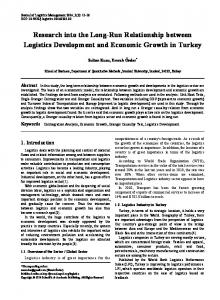
2. Data The set of time series data used in this paper consists of the daily closing indexes of the 5 emerging stock markets in ASEAN, namely VN-index, SET-index, KLSE-index, JKSE-index, and PSE-index, respectively representing for the stock markets of Vietnam, Thailand, Malaysia, Indonesia and the Philippines, and a series of international gold price based on the PM London Gold Fix (GoldFix, in short). As we know that working time of London gold market (local time) starts from 8:30 AM to 4:00 PM, of which the daily fixing prices are recorded twice at 10:30 AM and 3:00 PM and they can be used as the benchmarks for the official gold trading around the world. The sample period is selected from July 28, 2000 through March 31, 2009. The reason to select the starting time in the sample period is that the Vietnam stock market, a new established stock market, started opening the first trading on that day. The daily closing data of the five indexes were downloaded from Reuter, while the daily data of the PM London Gold Fix were obtained from website, http://www.kitco.com. In this study, daily prices at the PM London Gold Fix per ounce are expressed in the international standard currency (USD), while daily data of the five stock market indexes are expressed in domestic currencies to avoid the problem associated with price transmission due to fluctuations in cross-country exchange rates and also to avoid the restrictive assumption that relative purchasing power parity holds (Kasa, 1992). Other studies of Alexander and Thillainathan (1995), and Alexander (2001) also support for the idea that local currency should be used in testing cointegration. Figure 2 shows the plots of the selected price index series. Intuitively, there is a slightly up trend and down trend together in all the series over the sample period. 4000 3500 3000 2500 2000 1500 1000 500 0 1
104 207
310 413 516 619 722 825 928 1031 1134 1237 1340 1443 1546 1649
GOLDFIX
JKSE
KLSE
PSE
SET
VNI
Figure 2: The plots of the London Gold Fix and ASEAN emerging stock market indexes (28 July, 2000 to 31 March, 2009)
5
3. Econometric models To examine linkages among the sample markets, we employed the Johansen’s bivariate and multivariate cointegration tests (Johansen, 1988; Johansen and Juselius, 1990). The purpose of the test is to determine whether or not a group of non-stationary series is cointegrated. If the existence of cointegrating relation in the sample market price indexes is evident, there is a basis for forming the vector error correction models (VECM). Together with the Johansen test, we also perform unit root tests and the Granger causality test (Granger, 1969) for the data set.
Unit root tests
Prior to employing the Johansen technique, it is essential to test the order of integration in the data series used the study. Two most common methods, namely the Augmented Dickey Fuller (ADF) and Phillips and Perron (PP) tests for unit root are implemented for a set of the selected market price indexes, using the specification given in (1). The null hypothesis in the ADF and PP tests is that xt is non-stationary or is containing a unit root. p
∆xt = α0 + α1trend + ψ1xt-1 +
j xt j + ut
(1)
j 1
where ∆x is the first difference of xt and p is the lag-length of the augmented terms for xt. If the null hypothesis of a unit root in the level series is failed to reject, we conclude that the level series are nonstationary. However, if the null hypothesis of a unit root in the first differences of the level series can be rejected, these series are integrated of order one. Therefore, it is sufficient for performing cointegration tests for the level series.
Granger causality test
The Granger causality tests are applied to determine directions of causality between the market pairs. Since the Granger-causality test is very sensitive to the number of lags included in the regression, both the minimum Akaike information criteria (AIC) and Schwarz criteria (SC) should be considered to identify an appropriate lag length for each pair. The Granger causal relations are inferred through the generalized F statistic, which measures if the lagged terms of an exogenous variable significantly improve the autoregression of another. For instance, time series x1 is said to Granger-cause x2 if it can be shown the statistically significant information about future values of x2 through the F-test for the overall statistical significance of coefficients on the lagged values of x1 and x2 itself. Usually, causal relations are tested for both directions, from x1 to x2 and vice versa.
Johansen cointegration test
In our study, the long-run equilibrium relationship and the short-run dynamics among the six selected markets under the study are examined by employing the Johansen (1988) and Johansen & Juselius (1990) test framework. If the sample market price indexes have a common stochastic trend, then they are said to be cointegrated. Basically, cointegration of two or more variables implies a long-run equilibrium
6
relationship, given by the linear combinations between them, called the cointegrating vectors. If the presence of cointegrating vectors is evident in the test, there exists the VECM that measures speed of adjustment to the long-run equilibrium in the cointegrated variables. In order to test cointegration among the sample markets, we begin with a vector autoregressive (VAR) model of order p below p
xt = ω +
Ax i
t i
+ t
(2)
i 1
where xt is an (m x 1) vector of variables (x1t , x2t,…, xmt )’, which are m level series, ω is a vector of constants, Ai is a (m x m) matrix of coefficients and t is a vector of error terms, and p is the number of lags in the variables in the system. If the variables in the vector xt are integrated of order one, I(1), it implies that the linear combination of one or more of these series may exhibit a long-run relationship in (2). This leads to using the Johansen (1988) and Johansen & Juselius (1990) method for further explorations in the sample market price indexes. The method can be briefly expressed as follows p
Δxt = ω+
x i
t i
+ Пxt-1 + t
(3)
i 1
where xt is a (m×1) vector of the sample market price indexes, ω is the (m×1) vector of constant terms and εt is a vector of error terms. Гi denotes the (m×m) matrix of coefficients, containing information regarding the short-run relationships between the sample market price indexes. Meanwhile, П are (m×r) matrix, reflecting the possible long-run relationship between the sample market price indexes, where r is the rank of П so that r ≤ m −1. The Johansen procedure is to decompose the matrix П into two (m× r) matrices, α and β, such that Π = αβ'. The matrix β is called the matrix of cointegrating vectors, representing the possible long-run relationship between the sample market price indexes, and α is defined as the matrix of error correction coefficients that measure speed of adjustment in the variables to their long-run equilibrium. The Johansen technique is based on the maximum likelihood estimation of α and β' and the two computed statistics, namely the trace statistic and the maximum eigen-value statistic in order to test for the presence of r cointegrating vectors in the systems. The trace statistic tests the null hypothesis of at most q cointegrating vectors against the alternative hypothesis of r = n cointegrating vectors. The maximum eigenvalue statistic also tests for the presence of r cointegrating vectors against the alternative hypothesis of r+1 cointegrating vectors. For instance, if the null hypothesis (i.e., H0. r= 0 at the most) is failed to reject then stop the test, this means that there is no cointegrating relation among the system. On the contrary, if this null hypothesis is rejected, increase the value of r at the most and continue the test until the null hypothesis (i.e., H0. r=q at the most) can not be rejected. This indicates that there exist q cointegrating vectors in the system. Then, the VECM can be formed in the cointegrating relationships to measure speed of adjustment, for which the divergences of the endogenous variables in the system from their long-run equilibrium are controlled step by step to achieve the long-run equilibrium, while short-run dynamics remain unrestricted. In our study, the Johansen cointegration test procedure has conducted on the Eviews 6 econometric package software.
7
4. Empirical results In this section, we start with Augmented Dickey Fuller (ADF) and Phillips and Perron (PP) tests for the presence of a unit root in the time series data. Table 2 reports results of the tests. It indicates that the null hypothesis of the presence of a unit root in the 6 level series cannot be rejected, since all the t-statistics obtained from two methods are greater than the critical values at the 1%, 5% and 10% levels of significance. Therefore, nonstationarity exists in 5 stock market indexes and gold prices. However, the null hypothesis of a unit root in the first different (daily returns) series of the 6 market price indexes is clearly rejected, since all the t-statistics are less than the critical values. Therefore, these return series are stationary. In other words, all the level series of the selected markets are integrated of order one, I(1), implying that the linear combination or cointegrating relationship of one or more of these series may exhibit a long-run relationship. This satisfies the sufficient condition for the series of the selected stock market indexes and international gold prices to perform VAR and VEC methods. Table 2: Unit root tests for time series data of the sample markets Level series
First different
ADF
PP
ADF
PP
JKSE
-1,0633
-1,0132
-35,3578
-35,1234
KLSE
-1,0982
-1,1099
-36,7340
-36,8703
PSE
-1,1189
-1,1238
-39,4164
-39,3867
SET
-1,5598
-1,4097
-38,6609
-38,6636
VNI
-1,2833
-1,4081
-30,3913
-30,4501
GOLDFIX
-0,1902
-0,1902
-39,6778
-39,6791
Notes: Critical values at the 1%, 5% and 10% significant levels are -3.434, -2.863 and -2.568, respectively.
In order to investigate the causal relations between the selected stock market indexes and gold prices, we employ the Granger causality tests. Prior to conducting the test, it is necessary to identify the optimal lag length in each market pair. This can be done using VAR approach. For the optimum lag length selection, we use a maximum lag length of ten and perform VAR model in Eviews 6. Commonly, the two important information criteria such as Akaike information criteria (AIC) and Schwarz criteria (SC) are applied in many studies. This paper uses the optimal lag length suggested by SC for each market pair, which is based on the least value of SC among different lag lengths. The reason is that the optimal lag lengths suggested by SC for each pair are robust as we change the lag lengths, while those suggested by AIC are not so. Then Granger causality test for each pair can be conducted. Results of the Granger causality tests are reported in Table 3, and a summary of the significant directions of Granger causality between each pair is shown in Table 4.
8
Table 3: Granger causality test for the market pairs at the level series Ho
Lags
F-test
Ho
Lags
F-test
GOLDFIXJKSE
2
1.2384 (0.085)
PSEGOLDFIX
1
2.9065 (0.088)
GOLDFIXKLSE
1
2.4234 (0.120)
PSEJKSE
2
6.0801 (0.002)*
GOLDFIXPSE
1
1.2601 (0.262)
PSEKLSE
2
5.1434 (0.006)*
GOLDFIXSET
1
4.6033 (0.032)*
PSESET
2
5.5586 (0.004)*
GOLDFIXVNI
2
8.6072 (