Journal of Data Science 8(2010), 327-338
Combining Unsupervised and Supervised Neural Networks in Cluster Analysis of Gamma-Ray Burst Basilio de B. Pereira1 , Calyampudi R. Rao2 , Rubens L. Oliveira1,3 and Em´ılia M. do Nascimento1 1 Federal University of Rio de Janeiro, 2 Penn State University and AIMSCS and 3 Brazilian Naval Research Institute(IPqM) Abstract: The paper proposes the use of Kohonen’s Self Organizing Map (SOM), and supervised neural networks to find clusters in samples of gammaray burst (GRB) using the measurements given in BATSE GRB. The extent of separation between clusters obtained by SOM was examined by cross validation procedure using supervised neural networks for classification. A method is proposed for variable selection to reduce the “curse of dimensionality”. Six variables were chosen for cluster analysis. Additionally, principal components were computed using all the original variables and 6 components which accounted for a high percentage of variance was chosen for SOM analysis. All these methods indicate 4 or 5 clusters. Further analysis based on the average profiles of the GRB indicated a possible reduction in the number of clusters. Key words: Bayesian regularization, clustering and classification, cross validation, multilayer perceptron, self organizing map, supervised and unsupervised networks.
1. Introduction It is of great interest to astronomers to know whether the measurements on gamma-ray burst (GRB) can be characterized by a single probability distribution around some central value or as a mixture of probability distributions around different central values. Clustering is an exploratory data analysis (EDA) for investigating such problems by looking for groups of observed samples which are well separated using a suitable criterion. The ultimate aim is to seek for a physical interpretation of differences between the groups. An interesting example in a different context is the discovery of three clusters of the general population of individuals based on some blood tests for diabetes, one identified as diabetes free, and the other two representing individuals with 2 different types of diabetes A and
328
B.de B. Pereira et al. Table 1: Initial Variables
# ID 1 T50
Description
time measure representing the arrival of 50% of the flux 2 T90 time measure representing the arrival of 90% of the flux 3 F1 time-integrated fluence in spectral channels 20-50 keV 4 F2 time-integrated fluence in spectral channels 50-100 keV 5 F3 time-integrated fluence in spectral channels 100-300 keV 6 F4 time-integrated fluence in spectral channels over 300 keV 7 P64 peak flux measured in 64ms bins 8 P256 peak flux measured in 256ms bins 9 P1024 peak flux measured in 1024ms bind 10 T64 trigger threshold, i.e., number of counts in 64 ms required to trigger the second most brightly illuminated detector 11 T256 trigger threshold on the 256 ms timescale 12 T1024 trigger threshold on the 1024 ms timescale 13 Lat galactic latitude 14 Lon galactic longitude 15 FT sum of the four fluencies (F1 + F2 + F3 + F4) 16 H32 spectral hardness, obtained from fluence relation F3/F2 17 H321 spectral hardness, obtained from relation F3/(F1+ F2)
Mean of Log S.d. of Log 1.33
2.18
2.29
2.19
-15.61
2.11
-15.15
1.99
-13.94
1.82
-13.56
1.96
0.74 0.49 0.05 4.20
1.02 1.05 1.14 0.05
4.89
0.07
5.59
0.09
4.95 4.95 0.69
0.87 0.94 0.71
1.21
0.64
-12.62
1.71
B (Reaven and Miller, 1979). Another example is the discovery of 2 clusters of individuals suggesting 2 types of cancers (Golub et al., 1999). Cluster analysis is a valuable tool in knowledge acquisition. In the literature there are two approaches to cluster analysis. One is parametric assuming a mixture of a given number of probability distributions such as multivariate normal. Another is nonparametric which offers a great flexibility in discovering the number of clusters and their shape without going through model selection procedures. There are a number of methods of cluster analysis, a good review of which can be found in Jain, Murty and Flynn (1999) and Jiang et al. (2004). We use an unsupervised neural network known as SOM (Self Organizing Map) for finding
Unsupervised and Supervised Neural Networks
(a)
(b)
(c)
(d)
329
Figure 1: Clustering using Kohonen’s maps of 5 × 5 nodes (a), 7 × 7 nodes (b), 10 × 10 nodes (c), and 15 × 15 nodes (d)
clusters and discuss methods of validating them by cross validation and profile analysis. We also propose two methods of reducing the number of variables for obtaining stable results. Some references to early work on cluster analysis of GRB are Mitrofanov et al. (1998), Bagoly et al. (1998), Mukherjee et al. (1998), Hakkila et al. (2000), and Rajaniemi and Mahonen (2002). 2. Cluster Analysis 2.1 Data We consider the original BATSE 3B catalogue from the Compton Gamma Ray observatory, which is composed of 1122 GRB trigger samples with 14 measurements of astrophysical interest made on each sample. In addition we also list 3 other measurements usually considered in astrophysical research described in Murkerjee et al. (1998), Mitrofanov et al. (1998), Rajaneimi and Mahonen (2002). Since the computational complexity of the data mining process is not
330
B.de B. Pereira et al.
increased dramatically by including additional variables, we used all 17 variables. The list of 17 variables is given in Table 1 with the mean values and standard deviations of log variables. Log transformation is made to reduce the variables to uniform scale. 2.2 Cluster analysis using SOM There were 422 GRB samples with all variables present. A SOM was used for clustering these GRB patterns. Four different topologies were tried to test the clustering process. Figures 1a -1d show the number of patterns in each cluster over squared Kohonen’s map of different dimensions with nodes: 25(5×5), 49(7× 7), 100(10 × 10) and 225(15 × 15). As can be seen, the nodes representing the classes are well separated from each other in the 2 dimensional map provided by the topology. For a brief description of SOM and the underlying concepts, reference may be made to Rejaniemi and Mahonen (2000). All topologies clustered the 422 samples into 5 clusters designated as classes 1, 2, 3, 4 and 5. The fifth class had a small frequency and did not appear to be different from the fourth. They were combined to form one cluster as class 4. 2.3 Cross validation Working with the 15 × 15 topology (the one which presented the maximum relative distance between classes), the input patterns were divided into two groups called in sample set (317 patterns) and an out of sample set (105 patterns) with a random algorithm using stratified sampling. A supervised MLP (Multilayer Perceptron) neural net with Bayesian regularization (see Mackay, 1992) was used to train the in sample set for classification of patterns into four classes. Ten different trainings were performed and the patterns in the out of samples were classified into four classes. The overall mean accuracy of classification was 92.4% and the error for each class is as given in Table 2. Table 2: Misclassification error Classified as class
Belonging to class
1 2 3 4+5
1
2
3
4
47 2 2 0
2 14 0 0
2 0 33 0
0 0 0 3
Total
% Correct
51 16 35 3
92.15 87.50 94.28 100.00
It is seen that classes 1, 3 and 4 are well separated while 2 is not so well separated from 1. While this needs further discussion, we consider the four classes
Unsupervised and Supervised Neural Networks
331
to explain the method for reducing the number of variables. 2.4 Reduction of dimensionality In multivariate analysis, one is faced with the curse of dimensionality as originally pointed out by Rao (1952) and referred to in the statistical literature as Rao’s paradox. For obtaining stable results, a proper selection of variables has to be made. We suggest two procedures for this purpose, one of which is described in this section. The second is based on principal component analysis as detailed in the next section 3.
(a)
(b)
Figure 2: Relative importance of each input variable: (a) before pruning ( listed in table 1) and (b) after pruning (T50 , T90 , F1 , F2 , F3 , and F4 ).
Figure 2 (a) presents, for each input variable of the feedforward neural network, the sum of the absolute values of the weights (Si ) connecting the corresponding input to the hidden layer neurons. Taking the mean (M) and the standard deviation (SD) of theses sums and using as threshold (T) the value T = M − SD, we eliminated the variables whose Si were below T . The neural network was trained 10 times, for randomly chosen sets of the initial weights, and the pruning criterion was used to confirm the eliminated variables. The average of the misclassification error for these 10 samples will be denoted by AVj . After eliminating variables, further 10 training samples were used and the misclassification errors were computed. If the average of these errors (AVj+1 ) was more than the AVj value, then the variables would be definitively abandoned.The procedure is repeated iteratively until the elimination of variables does not improve the misclassification error. Figure 2 (b) shows the relative importance of each of the remaining input variables that were considered most relevant for the classification process (respectively T50 , T90 , F1 , F2 , F3 and F4 ). For this final configuration, the misclas-
332
B.de B. Pereira et al.
Figure 3: Percent of the total variability explained by each principal component.
sification error was 5.9% for the out of sample set and 1.4% for the in sample set). Considering six variables, the number of the available observations (without missing values) increased from 422 to 632. Using again a 15 × 15 topology for SOM, now for the six remaining input variables and for 632 patterns, the classes and frequencies found were similar to the classes obtained using all seventeen input variables. A feedforward neural network trained with the final six variables and 498 in sample and 134 out of sample observations resulted in an out of sample misclassification error of 5.9% compared with 7.6% with the 17 variables of the initial network with 317 in sample and 105 out of sample observations. However, considering that the objective is to compare this methodology with the next one (described in section 3), only the 422 patterns initially considered will be used to compare the two methods. 3. Principal Component Analysis A second approach to reduction of dimensionality is PCA (Principal Component Analysis) where the variables are replaced by a smaller number of linear functions of the variables. In computing the principal components only the first 14 variables of Table 1 are used. It may be noted that the last 3 variables of Table 1 are functions of the variables F1 , F2 , F3 , and F4 in the list. The computations made on 422 samples where all the variables are available provided 14
Unsupervised and Supervised Neural Networks
333
linear combinations of the variables with the associated eigen values as indicated in Figure 3. The first six principal components accounted for 98% of the total variance, and the SOM was used for clustering based on these components only. The analysis provided the same 5 classes as discussed in Section 2.
Table 3: Principal components according to PCA algorithm Variables
log T50 log T90 log F1 log F2 log F3 log F4 log P64 log P256 log P1024 log T64 log T256 log T1024 log Lon log Lat % variance % cumulative
Components 1st
2nd
3rd
4rd
5rd
6rd
0.414 0.432 0.441 0.420 0.374 0.299 0.060 0.097 0.169 0.000 0.000 0.001 0.020 -0.002 70.003 70.003
-0.449 -0.388 0.016 0.068 0.197 0.432 0.405 0.387 0.321 -0.001 0.000 0.002 -0.015 0.021 16.267 86.270
-0.103 -0.074 0.288 0.253 0.029 -0.823 0.210 0.231 0.246 -0.001 -0.001 -0.001 0.022 -0.001 5.150 91.421
-0.021 -0.049 0.079 0.063 -0.001 -0.005 -0.049 -0.052 -0.053 -0.004 -0.007 -0.013 -0.575 0.805 3.448 94.869
-0.033 -0.007 0.015 -0.009 -0.007 0.015 -0.035 -0.028 0.009 0.001 -0.001 0.002 0.815 0.577 1.983 96.852
-0.363 -0.355 0.513 0.337 0.039 0.086 -0.338 -0.370 -0.290 0.004 0.003 -0.007 0.048 -0.137 1.569 98.421
From the results of Table 3, we conclude that variables T50 , T90 , F1 , F2 , F3 and F4 are the most important. This result agrees with the previous one obtained using the MLP with a regularization technique which showed these same six variables as the most relevant to the classification process. Using this method, we obtained the same 5 classes of the previous analysis, with the same patterns in each class. The full table with the composition of each class is available from the authors. Labeling the classes found by SOM’s training process with numbers 1 to 5, it is possible to draw the patterns into graphs with the first versus the second and the third principal components provided by PCA analysis. These classes are clearly seen in Figure 4 and 5, where there is evidence of three classes (1,2 and 3). The status of classes 4 and 5 is not clear. However, some possibilities are that they may be considered as separate classes, class 5 may be merged with class 3, and 4 with 2. The profile analysis carried out in the next section also suggests similar grouping.
334
B.de B. Pereira et al.
Figure 4: Patterns classified by SOM projected in their 2 main principal components (supplied by PCA) – class 1 represented by ‘x’, class 2 by ‘•’, class 3 by star, class 4 by ‘o’ and class 5 by ‘¤’.
Figure 5: Patterns classified by SOM projected in their first and third principal components – class 1 represented by ‘x’, class 2 by ‘•’, class 3 by star, class 4 by ‘o’ and class 5 by ‘¤’.
4. Graphical Evaluation of the Classes There is no recommended statistical method as the best for evaluating the validity and the number of clusters determined by using one or more of the numerous algorithms available for cluster analysis. See Sugar and James (2003) and Jiang et al. (2004). Figure 6 gives the distortion curves recommended in
Unsupervised and Supervised Neural Networks
335
Sugar and James (2003), which suggests about 4 classes. Another suggested method is to examine the profiles of the patterns in different classes, which in statistical literature is also known as the plot of parallel coordinates of individuals and mean values as shown in Figure 7. It is seen that Classes 1 and 3 are distinct with class 2 occupying an intermediate position. The positions of classes 4 and 5 are not clear. It is interesting to see that the four classes differ mainly in mean values of the six variables chosen for clustering in Section 3.
Figure 6: Number of cluster x middle distance and distortion curve
6 5 4 3 2 1 0 1
2
3
4
5
6
7
8
9 10 11 12 13 14 15 16 17
-1 -2
Class 1
Class 2
Class 3
(a)
Class 4
Class 5
Class 1
Class 2
Class 3
Class 4
Class 5
(b)
Figure 7: Profiles and means. Panel (a): Parallel coordinate diagram, Panel (b): Means of variables (centralized for comparisons).
336
B.de B. Pereira et al.
5. Conclusion Our study indicates the following: a) The profile plot and the scatter plot of the first two principal components indicate a clear separation between Classes 1 and 3. Patterns in Class 1 are characterized by long duration, bright fluency and soft spectrum while Class 3, by short duration, faint fluency and hard spectrum. There is some overlap between Classes 1 and 2 in the profile plot, but the distinctiveness of Class 2 is brought out in the plot of principal components. Patterns in this class are characterized by intermediate duration and fluence, and hard spectrum. The positions of Classes 4 and 5 are not clear. However, the profile plots of classes 4 and 5 appear to be similar. Patterns in these classes can be characterized by intermediate duration, fluency and spectrum. b) The means of the variables T50, T90, F1, F2, F3, F4 and H321 of the 3 clusters are well differentiated while the means of the other 10 variables P64, P256, P1024, T64, T256, T1024, Lat, Lon, Ft and H32 are not. The latter variables may not be useful in predicting the class to which a future GRB belongs. Any physical interpretation of the clusters should take this into account. d) SOM seems to be an appropriate tool for clustering and graphical display of the results. e) The choice of the dominant principal components is a computationally convenient way of reducing the curse of dimensionality due to a large number of variables in cluster analysis and classification problem f) SOM provides non overlapping clusters and the distinction between the Classes 1 and 2 cannot be easily specified. A parametric approach such as fitting a mixture model may reveal three components as demonstrated in the paper by Mukherjee et al. (1998). References Bagoly, Z. et al. (1998). A principal component analysis of the 3B gamma-ray burst data. The Astrophysical Journal 498, 342-348. Golub, T. R. et al. (1999). Molecular classification of cancer: class discovery and class prediction by gene expression monitoring. Science 286, 531-537. Hakkila, J. et al. (2000). Gamma-ray class properties. The Astrophysical Journal 538, 165-180. Hoffman, P., Grinstein, G. and Pinkney, D. (1999). Dimensional anchors: a graphic primitive for multidimensional multivariate information visualizations. In Proceedings of the 1999 Workshop on New Paradigms in Information Visualization and
Unsupervised and Supervised Neural Networks
337
Manipulation in Conjunction with the Eighth ACM Internation Conference on Information and Knowledge Management (Kansas City, Missouri, United States, November 02 - 06, 1999). NPIVM ’99. ACM, New York, NY, 9-16. DOI= http://doi.acm.org/10.1145/331770.331775 Jain, A. K., Murty, M. N. and Flynn, P. J. (1999). Data clustering: a review. ACM Computing Survey 3, 264-323. Jiang, D., Tang, C. and Zhang, A. (2004). Cluster analysis for gene expression data: a survey. IEEE Transaction on Knowledge Discovery and Data Engineering 16, 1370-1386. MacKay, David J. C. (1992). A practical Bayesian framework for backpropagation networks. Neural Computation 4, 448-472. Mitrofanov, I. et al. (1998). Generic signatures of the time profiles of BATSE cosmic gamma-ray bursts. The Astrophysical Journal 504, 925-934. Mukherjee, S. et al. (1998). Three types of gamma ray bursts. The Astrophysical Journal 508, 314-327. Rao, C. R. (1952). Advanced Statistical Methods in Biometric Research. Wiley Rajaneimi, H. and Mahonen, P. (2002). Classifying gamma-ray burst using self-organizing maps. The Astrophysical Journal 566, 202-209. Reaven, G.M. and Miller, R. G. (1979). An attempt to define the nature of chemical diabetes using multidimensional analysis. Diabetologia 16, 17-24. Smyth, P. (1996). Clustering using Mont Carlo cross-validation. Proc 2nd International Conference on Knowledge Discovery and Data Mining AIII Press, 126-133. Sugar, A. and James, M. (2003). Finding the number of cluster in a data set :an information theorectical approach. Journal of the American Statistical Association 98, 750-763. Received April 30, 2009; accepted August 26, 2009.
338
B.de B. Pereira et al.
Basilio de B. Pereira Federal University of Rio de Janeiro Pos Graduate School of Engineering (COPPE) Faculty of Medicine and University Hospital Clementino Fraga Filho COPPE/UFRJ, CP 68507 , CEP 21941-972, Rio de Janeiro, RJ, Brazil basilio@hucff.ufrj.br Calyampudi R. Rao Penn State University and AIMSMS 326 Thomas Building, University Park, PA 16802,USA
[email protected] Rubens L. Oliveira Brazilian Naval Research Institute(IPqM) and Federal University of Rio de Janeiro Pos Graduate School of Engineering (COPPE) COPPE/UFRJ Caixa Postal 68506 - CEP: 21945-970 ,Rio de Janeiro - RJ, Brazil
[email protected] Em´ılia M. do Nascimento Federal University of Rio de Janeiro Pos Graduate School of Engineering (COPPE) COPPE/UFRJ CP 68507 , CEP 21941-972, Rio de Janeiro, RJ, Brazil
[email protected]