Jan 30, 2006 - David and Lucille Packard Foundation, and by Caltech's Lee Center for ...... distribution of channel magnitudes depends on the location of the.
Communication over a Wireless Network with Random Connections ∗ Radhika Gowaikar
Bert Hochwald
Babak Hassibi
Caltech
Bell Laboratories
Caltech
Pasadena, CA 91125
Murray Hill, NJ 07974
Pasadena, CA 91125
January 30, 2006
Abstract We analyze a network of nodes in which pairs communicate over a shared wireless medium. We are interested in the maximum total aggregate traffic flow possible as given by the number of users multiplied by their data rate. Our model differs substantially from the many existing approaches in that the channel connections in our network are entirely random: we assume that, rather than being governed by geometry and a decay-versus-distance law, the strengths of the connections between nodes are drawn independently from a common distribution. Such a model is appropriate for environments where the first order effect that governs the signal strength at a receiving node is a random event (such as the existence of an obstacle), rather than the distance from the transmitter. We show that the aggregate traffic flow as a function of the number of nodes n is a strong function of the channel distribution. In particular, for certain distributions the aggregate traffic flow is at least (lognn)d √ for some d > 0, which is significantly larger than the O( n) results obtained for many geometric models. Our results provide guidelines for the connectivity that is needed for large aggregate traffic. We show how our model and distance-based models can be related in some cases.
1 Introduction An early study of traffic flow in shared-medium wireless networks appears in the seminal work of Gupta and Kumar [11]. They show that in a grid network of n nodes on the plane having a deterministic power scaling ∗
This work is supported in part by the National Science Foundation under grant nos. CCR-0133818 and CCR-0326554, by the
David and Lucille Packard Foundation, and by Caltech’s Lee Center for Advanced Networking.
1
√ law, O( n) transmitters can talk simultaneously to randomly-chosen receivers. Similar results for networks with randomly-placed nodes can also be obtained (see, for example, [10] for a recent account). Different models can yield somewhat different conclusions [1, 3, 5, 9, 12, 14, 15, 16, 17]; nevertheless, if we do not permit the transmitter/receiver pairs to approach one another [6], or for very low attenuation laws [15], the model of a power decay law (as a function of distance) seems to yield a network in which the number of nodes that can talk simultaneously grows much slower than n. Network models that incorporate channel fading as well as geometric path loss have also been proposed [23, 22] but the scaling behavior of these is not much different from that of [11]. We wish to study networks with a different connectivity model. √ The O( n) result in [11] has the following heuristic explanation. If a node wishes to transmit directly √ to a randomly-chosen node (whose distance is approximately O( n) away on average), it has two choices: talk directly, or talk through a series of hops. If it tries to talk directly, the transmitter generates energy √ in a circle of radius O( n) around itself. However, this energy, which is seen by the intended receiver becomes interference for the O(n) other nodes in the circle. Thus, some fraction of the entire network of n nodes is bathed in interference; an undesirable consequence. If it decides instead to talk through hops, the √ transmitting node can pass its message to a neighbor, who in turn passes it to a neighbor and so on for O( n) √ hops to the intended receiver. This strategy limits interference to immediate neighbors but ties up O( n) √ nodes in the hopping process. Although this turns out to be the best strategy, only O( n) simultaneous messages can be passed before all n nodes in the network are involved. We change the model of the wireless medium from a model based on distance to one based on randomness. In multi-antenna links, a linear increase in capacity (in the minimum of the number of transmit/receive antennas) is obtained when the channel coefficients between the transmit and receive antennas are independent Rayleigh-distributed random variables [4, 13]. It is therefore now generally believed that a rich scattering environment, once thought to be detrimental to point-to-point wireless communications, may actually be beneficial. We show that a similar effect may hold for the expected aggregate data traffic in a wireless network; certain forms of randomness can be helpful. There are several reasons why one may choose a random model over one that is based on distance. While distance effects on signal strength are important for nodes that are very near or far from each other, many networks are designed with minimum and maximum distances in mind. Decay laws of the form 1/r m for a fixed m > 0 may not be relevant for networks of small physical size. Additionally, through the use of automatic gain control, a radio often artificially mitigates distance effects unless the node is saturated (too close) or “dropped out” (too far). Many first-order signal-strength effects in such networks are then due to 2
random fluctuations in the medium, such as Rayleigh and shadow fading. A distance-power model cannot readily account for shadow fading since signal strength at the receiver is determined more by the presence of an obstacle blocking the path to the transmitter than by distance. In addition, recent investigations show that the connectivity of ad hoc networks with channel randomness, such as that caused by shadow fading, is similar to the connectivity in a random graph [24]. Networks with spread out connections are studied in [25, 26] and the analysis of this indicates that geometric network models with some unreliability in the connections have many randomness properties that are missing in a purely deterministic model. These results are primarily concerned with the connectivity of the networks whereas in this paper we go one step further and propose a throughput analysis of a random model. We adopt the premise that randomness can have a first-order effect on the behavior of a network. We assume that the channels between nodes are drawn independently from an identical distribution. We allow the distribution of the channel between nodes to be arbitrary and allow it to vary with the number of nodes n. Our model covers environments where the the signal strength at a receiving node is governed primarily by a random event (such as the existence of an obstacle). This model was first presented in [27]. We believe that the study of such wireless networks with random connections is important for three reasons: first, many real wireless networks have a substantial and dominant random component; second, we show that such networks may have qualitatively different traffic scaling laws than the scaling obtained in geometric models; finally, our results give insight into the connectivity that a network should have to allow large aggregate traffic flows. In general, any realistic model of a large network should have a model of connectivity that has a balance of randomness and distance-based effects. In [28] one such model is proposed and its throughput is analyzed. Also, [8] uses a “radio model” to show that in the presence of obstructions and irregularities, channels become approximately uncorrelated with one another, and the probability of good links between nodes that are far apart increases in wireless local area networks (WLANs). The radio model in [8] essentially uses the same independence assumption that we do, but uses distance to determine the probability of a connection link. We show in Section 8.1.1 how to apply our traffic-flow conclusions to this radio model to determine a favorable distance between nodes.
1.1 Approach We suppose that the connection strengths between the n nodes of the wireless network are drawn independently and identically from a given arbitrary distribution. In geometric networks such as [11] a node may communicate its message in hops to nearby neighbors so that it ultimately reaches the intended destination. 3
In our random model, although there is no geometric notion of a near neighbor, we can find an equivalent of a near neighbor by introducing the notion of “good paths”, where connections stronger than a chosen threshold β are called good. Transmissions to relays and destinations occur along only good paths. By figuratively drawing a graph whose vertices are all the nodes in the network, yet whose edges are only the good paths, we obtain a specific random graph model called G(n, p), where an edge between any pair of
the n nodes exists with probability p. (In our case, p is simply the probability that the connection strength
exceeds βn .) G(n, p) is a very well-studied object and we leverage some of its known properties to establish
disjoint routes between sources and their intended destinations. However since we are analyzing a wireless network, we must also account for the effects of interference between all nodes, including those that do not have good connections between them. Fortunately, our use of the goodness threshold β also makes the analysis of message-failures (due to interference and/or noise) tractable. Our analysis yields an achievable aggregate throughput which is a function of the chosen threshold β. A judicious choice of β can maximize this achievable throughput. To complement our achievability results, we also present on some upper bounds on aggregate throughput that show that our results are sometimes tight.
2 Model of Transmitted and Received Signals We assume that the wireless network has narrowband flat-fading connections whose powers are independent and identically distributed (i.i.d.) according to an arbitrary distribution f (·). Thus, if h i,j is the connection between nodes i and j, then the γi,j = |hi,j |2 are i.i.d. random variables with marginal distribution f (γ i,j ).
For maximum generality, we allow f (γ) = f n (γ) to be a function of the number of nodes n. As an example, consider f (γ) = (1 − p) · δ(γ) + p · δ(γ − 1)
(1)
where δ(·) is the Dirac delta-function. This distribution is a simple model of a shadow-fading environment where, for any pair of nodes, with probability p there exists a good connection between them (fading causes no loss), and with probability 1 − p there exists an obstruction (fading causes a complete loss). In a general
network of n nodes, we may let p = pn be a function of n to represent changes in the geography or network topology as the network increases in size. Although γ = 0 and γ = 1 are the only possibilities in the distribution (1), we may also introduce values of γ that depend on n. Figure 1 pictorially displays an example of wireless terminals whose connections may obey the model (1). The behavior of such a network varies dramatically with p. At the extreme of p = 1 no paths are ever 4
Figure 1: Nodes are able to establish connections with each other if there is no object in their path. Equation (1) models the presence of an object as a random event where each path has a connection of strength one with probability p, and otherwise has a connection of strength zero.
5
blocked and all nodes are fully connected to each other. While this situation permits any node to readily talk to any other node in a single hop, the overall network throughput is low because talking pairs generate an enormous amount of interference for the remaining nodes. If many nodes try to talk simultaneously, the overall interference is overwhelming. At the other extreme of p = 0, everyone is in a deep fade; now interference is minimal. However, no nodes can talk at all (we assume a transmission power limit). Thus we have competing effects as a function of p: increasing p benefits the network by improving connectivity thus allowing for shorter hops, but hurts the network by increasing interference to other receivers. We are led to ask: what p is optimal? What is the resulting network aggregate traffic? Is this optimal p likely to be something we encounter naturally? If not, can we induce it artificially? We answer some of these questions but, more generally, we look at how an arbitrary f n (γ) affects the traffic.
2.1 Detailed model Let the network have n nodes labeled 1, . . . , n. Every pair of nodes {i, j} (i 6= j) is connected by a channel � that is denoted by the random variable h i,j = hj,i ; there are n2 channel random variables. The channel
strengths, γi,j = |hi,j |2 are drawn i.i.d. according to the probability density function (pdf) f n (γ). Once drawn, these channel variables do not change with time.
Node i wishes to transmit signal xi . We assume that xi is a complex Gaussian random process with zero mean and unit variance. Each node is permitted a maximum power of P watts. We incorporate interference and additive noise in our model as follows. Assume that k nodes i 1 , i2 , . . . , ik are simultaneously transmitting signals x i1 , xi2 , . . . , xik respectively. Then, the signal received by node j(6= i1 , . . . , ik ) is given by yj =
k √ X P hit ,j xit + wj
(2)
t=1
where wj represents additive noise. The additive noise variables w 1 , . . . , wn are i.i.d., drawn from a complex Gaussian distribution of zero mean and variance σ 2 (wj ∼ CN (0, σ 2 )). The noise is statistically independent of xi .
6
2.2 Successful communication In equation (2), suppose that only node i 1 wishes to communicate with node j and the signals x i2 , . . . , xik are interference. Then the signal-to-interference-plus-noise ratio (SINR) for node j is given by ρj =
P γi1 ,j P σ 2 + P kl=2 γil ,j
We assume that transmission is successful when the SINR exceeds some threshold ρ 0 . If the SINR is less than ρ0 , we say that transmission is not possible. Thus, any successful transmission occurs at a rate of at least log(1 + ρ 0 ). The rate can actually be upto log(1 + ρ) where ρ ≥ ρ0 is the precise SINR. However, the rate that is guaranteed for each transmission is
only log(1 + ρ0 ). Therefore we will use log(1 + ρ0 ) as the transmission rate. This will be the actual rate if we assume that all transmissions occur at this rate only. Alternatively, if transmissions at other rates are permitted, we can think of log(1 + ρ0 ) as a conservative estimate of the rate of information flow. Finally, using log(1 + ρ0 ) as the rate for each communication rather than the more precise log(1 + SINR) simplifies the analysis of a throughput guarantee considerably. Therefore, we will use log(1 + ρ 0 ) as the rate in the rest of the paper. In simulations presented at the end, however, we present plots where the precise rate at which communications can occur is considered, since this is more relevant from a practical point of view.
3 Network Operation and Objective We suppose that k nodes, denoted by s 1 , . . . sk , are randomly chosen as sources. For every s i , a destination node di is chosen at random, thus making k source-destination pairs. We assume that these 2k nodes are all distinct and therefore k ≤ n/2. Source s i wishes to transmit message Mi to destination di and has encoded it as signal xi . We wish to see how many source-destination pairs may communicate simultaneously. The sources may talk directly to the destination nodes or may decide to communicate in hops through a series of relay nodes.
3.1 Communicating with hops In general, we suppose that the source-destination pair (s i , di ) communicates using a sequence of relay nodes ri,1 , ri,2 , . . . , ri,h−1 . (h = 1, 2, . . . represents the number of hops.) Define r i,0 = si and ri,h = di . The path from si to di is then ri,0 = si , ri,1 , ri,2 , . . . , ri,h−1 , ri,h = di . In time slot t + 1 we have nodes r1,t , r2,t , . . . , rk,t transmitting simultaneously to nodes r 1,t+1 , r2,t+1 , . . . , rk,t+1 respectively. We ask that 7
nodes r1,t+1 , r2,t+1 , . . . , rk,t+1 decode their respective signals x1 , x2 , . . . , xk and transmit them to the next set of relay nodes in the (t + 2)th time slot, and so on. A natural condition to impose is that the relay nodes that are receiving (or transmitting) messages in any time slot be distinct; the messages do not collide. In addition, we ask that relay nodes not receive and transmit at the same time. We refer to these conditions together as the property of no collisions in the rest of the paper. In general, we do not require r i,t to be distinct from ri,t+1 for any i. This means that a relay can effectively hold on to a message in a time slot; hence h effectively represents the maximum number of hops needed for all the source-destination pairs. s1
r1,1
r1,2
r1,h−1
d1
s2
r2,1
r2,2
r2,h−1
d2
sk
rk,1
rk,h−1
rk,2
dk
Figure 2: Schedule of relay nodes: Source s i communicates with destination di using relays ri,1 , . . . , ri,h−1 . The solid lines indicate intended transmissions and the dashed lines indicate potential interference. A schedule is valid if it meets the no-collision conditions that a node can receive or transmit at most one message in any time slot and that no node can transmit and receive simultaneously.
3.2 Throughput With the above procedure, we have k simultaneous communications occurring in h time slots. Message Mi reaches the intended destination d i successfully if it can be decoded by each relay r i,t . Assume that a fraction 1 − � of messages reach their intended destinations in this way. Then, we define the throughput as k T = (1 − �) log(1 + ρ0 ), h
(3)
where ρ0 is the SINR threshold, and we are using the natural logarithm. Thus, log(1 + ρ 0 ) is the sustainable throughput per user if the users do not collide, as mentioned in Section 2.2. We multiply this factor by the number of non-colliding source-destination pairs k, divide by the number of hops, and subtract the fraction of dropped messages �. The resulting throughput T depends on n and we sometimes add subscripts to the variables involved to indicate this: k n , �n , ρ0,n and Tn . Typically, we force �n to go to zero as n grows. We demonstrate a scheme for choosing the relay nodes and analyze the throughput performance of this scheme. 8
Thus, we give an achievability result for T n . We now state this result.
4 Main Result Theorem 1. Consider a network on n nodes whose edge strengths are drawn i.i.d. from a probability distribution function fn (γ). Let Fn (γ) denote the cumulative distribution function corresponding to f n (γ) and define Qn (γ) = 1 − Fn (γ). Choose any βn such that Qn (βn ) =
log n+ωn , n
where ωn → ∞ as n → ∞.
Then there exists a positive constant α such that a throughput of log(nQn (βn )) T = (1 − �n ) αkn (βn ) log 1 + log n
an βn σ2 P
+ (kn (βn ) − 1)µγ
!
(4)
is achievable for any positive an such that an ≤ 1 and any kn (βn ) that satisfy the conditions: 1. kn (βn ) ≤ αn 2. �n ≤
log(nQn (βn )) log n
(5)
(kn (βn ) − 1)σγ2 log n a2n →0 2 2 σ 2 α(1 − an ) ( + (kn (βn ) − 1)µγ ) log(nQn (βn )) P
where µγ and σγ2 are the mean and variance of γ respectively. The SINR threshold ρ 0 is given by The parameter βn satisfying Qn (βn ) =
log n+ωn n
(6) an β n σ2 +(k (βn )−1)µγ n P
is the goodness threshold mentioned in Section 1.1.
By figuratively drawing an edge when γ > β n , we obtain a random graph that fits the well-studied model G(n, p). Condition (5) is needed to obtain a non-colliding schedule in this random graph. This issue is discussed in detail in Section 5. Once the schedule is obtained, we incorporate the effects of interference
between non-colliding transmissions and provide an error analysis in Section 6. Condition (6) forces � n to go to zero. In Section 7 we combine the results of Sections 5 and 6 to prove the theorem. Note that the theorem indicates an achievable throughput and does not preclude that higher throughputs are possible. Although not evident from the theorem statement at this time, it turns out that the optimum number of hops h grows at most logarithmically with n. The throughput therefore depends most strongly on the number of simultaneous transmissions k n and the SINR threshold ρ0 . The throughput expression (4) is general and accommodates an arbitrary f n (γ). The parameter kn is the number of non-colliding simultaneous transmissions. We discuss the constant α and the parameter a n later. The joint selection of βn , kn , and an that maximizes the achievable throughput (4) is not easily expressed 9
.
in closed-form as a function of the pdf f n (γ). In general, these parameters need to be determined on a case-by-case basis. We show how to find the necessary parameters in Section 8 where we give several examples. Since (4) holds for any kn satisfying (5), we may choose kn as large as possible (achieving equality in (5)) and optimize only over an and βn . In fact, when
σ2 P
− µγ ≥ 0, it is possible to show that the optimum
kn is the maximum possible. We hence state a more specific achievability result. Corollary 1. In the network of Theorem 1, if
σ2 P
− µγ ≥ 0 the throughput (4) is maximized by choosing k n
as large as possible. At this point we would like to refer back to the problem setting of [11] and note that their model of a random network, where nodes wish to send information at the rate of λ(n) bits per second to a randomly chosen destination is closest to the problem we consider here. For the random network, an aggregate p throughput capacity of O( n/ log n) is obtained in [11]. (This is only slightly worse than the transport √ capacity of O( n) for the somewhat different model of arbitrary networks, which has been discussed in the introduction to this work.) In the example presented in Section 8.2 we examine the scaling behavior of the throughput with a pdf fn (γ) that is obtained based on a distance-decay law. The effects of doing away with the geometric model become more clear with that example.
5 Scheduling Transmissions With a view to meeting a minimum SINR of ρ 0 at every relay node at every hop, we impose the condition that each transmitting link be stronger than some threshold β n . We require that γri,t ,ri,t+1 ≥ βn , where βn
is a design parameter. We denote links that satisfy γ i,j ≥ βn as good. We require the path from si to di to
use only good links.
The threshold βn is a parameter that we may choose as a compromise between quantity and quality of the connections. By making βn large we increase the quality of the link. However, if we make it too large we risk not being able to form an uninterrupted path of good links from the source to the destination. In this section, we determine the relation between β n and the lengths of source-destination paths. Define pn = P(γ ≥ βn ) (for convenience, we drop the subscript n in the rest of this section). Using
our wireless communication network, we define a graph on n vertices as follows: For (distinct) vertices i
and j of the graph, draw an edge (i, j) if and only if γ i,j ≥ βn in the network. Call the resulting graph G(n, p). The graph G(n, p) then becomes an instance of a model called G(n, p) on n vertices in which 10
edges are chosen independently and with probability p [2]. This graph shows the possible paths from the various sources to the various destinations using only good links, but does not show the possible interference encountered if these paths are used simultaneously. We examine this interference in Section 6. Graphs taken from the model G(n, p) have many known properties. For instance, the values of p for
which the graph is connected is well-characterized. As p increases the probability that the graph is connected goes to one. If p = connected is e
−e−c
log n+c+o(1) n
(where c > 0 need not be a constant) the probability of the graph being
[2]. This implies that there is a phase transition in the graph around p =
log n n .
For p
less than this the probability of connectivity goes to zero rapidly and for p greater than this it goes to one rapidly. Another property that is well-studied is the diameter. The diameter of a graph is defined as the maximum distance between any two vertices of the graph, where the distance between two vertices is the minimum number of edges one has to traverse to go from one to the other. Results in [2] and [18] tell us that for p in the range of connectivity the diameter behaves like
log n log np .
(It is also known that the average distance
between two nodes has the same behavior.) This tells us that a message can be transmitted from one node to another using at most
log n log np
hops. What it leaves unanswered is the question of how to establish k such
transmissions simultaneously and on non-colliding paths. The problem of obtaining a non-colliding schedule can be thought of more generally as a problem of avoiding or reducing interference. Not surprisingly, several works that study throughput scaling in large networks encounter the same issue, irrespective of the precise network model being employed. For instance, in [11] the number of routes that pass through a certain small area of the network (which they call a cell) can be thought of as the bottleneck that determines the overall throughput. Similarly, in [10], the number of disjoint paths that can be found in a certain area can be perceived as the limiting factor. Various techniques are used in these works to enable this calculation. While [11] uses results relating to the Vapnik-Chervonenkis dimension, [10] uses ideas inspired by percolation theory and random geometric graphs [29]. In the setting of this work, it is most natural to use random graph theory and we use a relatively recent result regarding vertex-disjoint paths by Broder et al [19] in order to find a satisfactory non-colliding schedule.
5.1 Scheduling using vertex-disjoint paths in G(n, p) Two paths that do not share a vertex are called vertex-disjoint. Note that any two paths that are vertex-disjoint satisfy our “no-collisions” property; however, the reverse statement is not true. Thus, the vertex-disjoint condition is stronger than our requirement of non-colliding paths. For a set of k (disjoint) pairs of vertices (si , di ), the question of whether there exists a set of vertex-disjoint paths connecting them is addressed in 11
[19]. Their result states that with high probability, for every (sufficiently random) set of k pairs (s i , di ) and np k not greater than α1 n log log n , where α1 is a constant, there exists a set of vertex-disjoint paths. This result is
within a constant of the best one can hope to achieve since the average distance between nodes in G(n, p) is log n log np ,
np and thus we can certainly have no more than n log log n vertex-disjoint paths. Also stated in [19] is an
algorithm that finds k paths using various random walk and flow techniques. Here we reproduce their main result. Theorem 2. Suppose that G = G(n, p) and p ≥
log n+ωn , n
where ωn → ∞. Then there exist two positive
constants α1 , α2 such that, with probability approaching 1, there are vertex-disjoint paths connecting s i to di for any set of pairs F = {(si , di )|si , di ∈ {1, . . . , n}, i = 1, . . . , k} satisfying 1. The pairs in F for i = 1, . . . , k are disjoint; np 2. The total number of pairs, k = |F |, is not greater than α 1 n log log n .
3. For every vertex v ∈ {1, . . . , n}, no more than a α 2 -fraction of its set of neighbors, N (v), are prescribed endpoints, that is |N (v) ∩ (S ∪ D)| ≤ α 2 |N (v)|, where S = {si } and D = {di }. Furthermore, these paths can be constructed by an explicit randomized algorithm in polynomial time. In fact, the existence of the paths is proved by stating and analyzing a randomized algorithm that finds them. However, we use this theorem only as an existence result to demonstrate achievable throughputs. Some comments about their randomized algorithm can be found in Sections 6 and 10.1. In our communication network, Condition 1 that (s i , di ) be disjoint pairs is already met. The second imposes a restriction on how large k can be. Since the k source-destination pairs are chosen at random, the third condition is also met. (In fact, the third condition is imposed in [19] to prevent someone from choosing the (si , di ) pairs in a particularly adversarial manner using knowledge of the graph structure.) We can restate the theorem for our purposes. Theorem 3. Suppose that G = G(n, p) and p ≥
log n+ωn , n
where ωn → ∞. Then there exists a constant
α > 0 such that, with probability approaching 1, there are vertex-disjoint paths connecting s i to di for any set of disjoint, randomly chosen source-destination pairs F = {(si , di )|si , di ∈ {1, . . . , n}, i = 1, . . . , k} 12
np provided k = |F | is not greater than αn log log n .
The constant α in this theorem is the same α required in Theorem 1. It is not explicitly specified. We examine the lengths that these k paths can have in the following lemma. np Lemma 1. Almost all of the k = αn log log n vertex-disjoint paths obtainable under Theorem 3 have lengths
that grow no faster than
log n α log np .
Proof. Suppose that some fraction of paths, say c n k where cn > 0 have average lengths of the form log n log np (1
+ ωn0 ) where ωn0 goes to infinity. Since there are n nodes in the network, we have n ≥ cn k ×
log n log np log n (1 + ωn0 ) = cn αn × (1 + ωn0 ) = cn αn(1 + ωn0 ). log np log n log np
This implies that 1 ≥ αcn (1 + ωn0 ) and therefore cn must go to zero. Therefore we conclude that at most a vanishing fraction of the k paths can have lengths that grow faster than
paths have lengths that grow no faster than
log n log np
and, asymptotically, all the
log n α log np .
Hence the number of hops h is (asymptotically) at most
log n α log np .
We use this fact in the error analysis in
the following section.
6 Probability of Error np Consider a schedule of k ≤ αn log log n non-colliding paths. Theorem 3 shows that such a schedule exists.
One possible (but often impractical) way to obtain such a schedule is to use an exhaustive search that first lists all the paths between every source-destination pair and then randomly chooses a set that satisfies the
vertex-disjoint property. Because we thereby choose a path based on vertices rather than edges, we are assured that any edges that might exist between vertices along one path to vertices along another are i.i.d. Bernoulli distributed with parameter p. We also conclude that the channel connections between nodes along different paths in the network are i.i.d. with distribution f n (γ). More generally, randomized algorithms that choose non-colliding paths without using edge information between such paths also have the property of generating i.i.d. interference between the paths. An example of such a randomized algorithm that avoids an exhaustive search is [19]. We now consider the probability that a particular message fails to reach its intended destination. Destination di fails to receive message Mi if the SINR falls below ρ0 at any of the h relay nodes ri,1 , . . . , ri,h = di .
13
Denote by Et the event that relay node ri,t does have an SINR greater than ρ0 . Note that the events E1 , . . . , Eh are identical. Therefore we have, P(Mi is received successfully) = P(
h \
t=1
Et ) = 1 − P(
h [
t=1
∼ Et ) ≥ 1 −
h X t=1
P(∼ Et ) = 1 − hP(∼ E1 ) (7)
where the inequality comes from the union bound. We now compute P(∼ E 1 ). This is the event that node ri,1 has an SINR lower than ρ0 P(∼ E1 ) = P(ρri,1 ≤ ρ0 ) = P
P γsi ,ri,1 P ≤ ρ0 2 σ + P j6=i γsj ,ri,1 γsj ,ri,1 ≥
≤ P
X
γsj ,ri,1
j6=i
j6=i
σ2
P γsi ,ri,1 − ρ0 P ρ0 2 P βn − ρ0 σ ≥ P ρ0
= P
X
!
σ2
P βn − ρ0 1 γsj ,ri,1 − µγ ≥ − µγ k−1 (k − 1)P ρ0 j6=i 1 X P βn − ρ0 σ 2 ≤ P − µγ γsj ,ri,1 − µγ ≥ (k − 1)P ρ0 k − 1
= P
X
j6=i
≤
σγ2 /(k − 1) βn −ρ0 σ 2 2 ( P(k−1)P ρ0 − µγ )
(8)
where the first inequality is because γ si ,ri,1 ≥ βn and (8) comes from the Chebyshev inequality and the 1 P 2 fact that the variance of k−1 j6=i γsj ,ri,1 is σγ /(k − 1). The second inequality requires the condition P βn −ρ0 σ 2 (k−1)P ρ0
− µγ ≥ 0, or
ρ0 ≤
βn σ2 P
+ (k − 1)µγ
.
(9)
This condition on ρ0 is intuitively satisfying: if we assume that k is large, then we expect the interference term in the denominator of the SINR to be approximately (k − 1)µ γ . This would imply that setting
the threshold ρ0 to less than threshold.
βn σ2 +(k−1)µγ P
would be sufficient to ensure that most hops would exceed this
Note that in the above analysis for P(ρ ri ,t ≤ ρ0 ), we have assumed that there are (k − 1) interference
terms. This would be true if all k messages are being transmitted in that particular time slot. However, this may not be the case, if, by that time slot, some of the messages have already reached their destinations 14
successfully or have already failed to be decoded at some at some relay node. In such a case, there will be fewer than (k − 1) interference terms. This means that the calculation above is conservative and the actual probability of error may be smaller than that obtained above. However, from the relevant theory involving
random graphs as well as from the simulations, we expect the path lengths to cluster quite densely rather than taking on a wide range of values. Thus, most messages reach their destination within very few time slots of each other. Therefore, we believe that the above error analysis is not too conservative and hence do not expect a significantly lower error probability in practice. We define �n to be the probability that the SINR threshold is not exceeded along one or more of the hops. From (7), �n ≤ hP(∼ E1 ). We force hP(∼ E1 ) to go to zero. From Lemma 1, h is at most
and we have
�n ≤ hP(∼ E1 ) ≤
log n α log np
σγ2 log n α log np (k − 1)( P βn −ρ0 σ2 − µγ )2 (k−1)P ρ0
(10)
and we require the right-hand side to go to zero.
We mention that the inequality (10) requires γ to have a variance that does not go to infinity. There are several distributions of practical interest in which the variance does go to infinity, but the mean is finite. (For example, f (γ) =
c (1+γ)m
for m > 2 is considered in [28].) In this case, an alternative inequality can be
obtained by applying the Markov bound to P(∼ E 1 ) rather than the Chebyshev bound . The result is �n ≤ hP(∼ E1 ) ≤
log n (k − 1)µγ P ρ0 . α log np P βn − ρ0 σ 2
(11)
An achievable throughput can be obtained using either the Chebyshev bound of (10) or the Markov inequality above. The result of Theorem 1 is obtained using the Chebyshev inequality. In Theorem 4, presented at the end of Section 7, we state an achievability result obtained using the Markov inequality of (11). In general, we expect the Chebyshev inequality to be tighter than the Markov inequality and therefore prefer to use Theorem 1 rather than Theorem 4 whenever we can.
7 Proof of Theorem 1 We now combine the results of Section 5 on the maximum number of non-colliding paths and Section 6 on the probability of successful transmission along these paths. We need p = P(γ ≥ β n ) = Qn (βn ) = log n+ωn n
in order to do scheduling. In addition, we need:
1. To have non-colliding paths (Theorem 3) k ≤ αn 15
log np log n
2. To meet the SINR threshold (equation (10)) �n ≤
σγ2 log n →0 α log np (k − 1)( P βn −ρ0 σ2 − µγ )2 (k−1)P ρ0
3. To apply the Chebyshev inequality (equation (9)) ρ0 ≤
βn σ2 P
+ (k − 1)µγ
To satisfy the third condition above we set ρ0 =
an βn σ2 P
+ (k − 1)µγ
where 0 ≤ an ≤ 1. Substituting for this in the second condition, we get �n ≤
(kn (βn ) − 1)σγ2 a2n log n → 0. 2 2 σ 2 α(1 − an ) ( + (kn (βn ) − 1)µγ ) log(nQn (βn )) P
This and the first condition above are the only conditions on k. For any k satisfying these two conditions we get an achievable throughput. This gives us Theorem 1. The theorem gives an achievable throughput as a function of β n , an and kn but does not attempt to optimize these parameters. Because � n goes to zero and h is determined by βn , to find the optimum k we need to maximize k log(1 + ρ0 ) = k log(1 +
an β n σ2 +(k−1)µ γ P
) over k. In the particular case when
σ2 P
− µγ
is positive, the expression is non-decreasing in k (the first derivative is non-negative). Hence satisfying (5) with equality is optimum. This proves Corollary 1. Finally, we state without proof an achievability result obtained using (11) to bound the error, rather than (10). This result can be used in place of Theorem 1 for distributions that have a finite mean but an infinite variance.
Theorem 4. Consider a network on n nodes whose edge strengths are drawn i.i.d. from a probability distribution function fn (γ). Let Fn (γ) denote the cumulative distribution function corresponding to f n (γ) and define Qn (γ) = 1 − Fn (γ). Choose any βn such that Qn (βn ) =
log n+ωn , n
where ωn → ∞ as n → ∞.
Then there exists a positive constant α such that a throughput of log(nQn (βn )) T = (1 − �n ) αkn (βn ) log 1 + log n
βn σ2 P
+ bn (kn (βn ) − 1)µγ
!
is achievable for any positive bn such that bn ≥ 1 and any kn (βn ) that satisfy the conditions: 16
(12)
1. log(nQn (βn )) log n
(13)
log n 1 →0 αbn log(nQn (βn ))
(14)
kn (βn ) ≤ αn 2. �n ≤
where µγ is the mean of γ. The SINR threshold ρ 0 is given by
βn σ2 +b (k n n (βn )−1)µγ P
.
8 Examples and Applications In this section we apply Theorem 1 to some particular channel distributions. Since, as in geometric models, the throughput is often interference-limited, we find that densities that lead to significant interference per transmitter generally underperform those that generate only a small amount of interference.
8.1 Shadow fading model We revisit the model (1) (15)
fn (γ) = (1 − pn )δ(γ) + pn δ(γ − 1)
where δ(·) is the Dirac delta-function. This pdf models the situation where strong shadow fading is present. The signal power is 0 in the presence of an obstruction and is 1 otherwise. We find the value of p that maximizes the throughput. (We drop the subscript n.) A natural choice for the goodness threshold β n is 1, which gives Q(β) = p. We need to satisfy p ≥ (log n + ω n )/n (where ωn → ∞) in order to use Theorem 1.
Note that we have µγ = p and σγ2 = p(1 − p). It is possible to check that unless p → 0, the throughput
is at most constant. With p → 0 and sufficiently large n, the condition
σ2 P
− µγ =
σ2 P
− p ≥ 0 is satisfied.
Therefore, according to Corollary 1 the maximum possible k achieves maximum throughput. Hence we np consider k = αn log log n . Since p =
log n+ωn , n
k → ∞ and we may replace k − 1 by k in (6) and the SINR
threshold. Since kp also goes to infinity, (6) becomes � n ≤
a2n log2 n 1 α2 (1−an )2 log2 (np) n
any positive constant a < 1. With this, the SINR threshold becomes ρ 0 =
goes to zero. Thus log(1 + ρ0 ) ≈ ρ0 and we have
as small as possible, or p =
log n+ωn . n
k h
log(1 + ρ0 ) =
a
np σ2 +αnp log P log n
aα log np p log n .
≈
a np αnp log log n
which
This is maximized when p is
The result is summarized in the Corollary.
17
→ 0. Therefore an may be
Corollary 2. Consider a network on n nodes where edge strengths are drawn i.i.d. from the distribution in n and is given by (15). Then for large n the throughput is maximized for p = log n+ω n � � a2 log(log n + ωn ) 1 log2 n T = 1− 2 aα n 2 2 α (1 − a) log (log n + ωn ) n (log n + ωn ) log n
as n → ∞, where ωn is any function going to infinity and 0 < a < 1 and α < 1 are constants. This throughput is almost linear in n and requires the network to be sparsely connected; with a connection probability of (log n)/n, each node is connected with only approximately log n other nodes. For example with n = 1000 nodes, we have (log n)/n = 0.0069 and each node connects on average to only seven other nodes. Perhaps surprisingly, increasing or decreasing this connectivity has a detrimental effect. While it is clear that it is possible for a network to be under-connected, it is apparently also possible for a network to be over-connected. The simulations in Section 10.2 also demonstrate this effect. 8.1.1
Implications for a certain radio model
In [7, 8] a wireless connectivity model is introduced where the probability of a good link is expressed as � � �� log rˆ 1 1 − erf 3.07 (16) p(ˆ r) = 2 ξ where rˆ is a (suitably normalized) distance between the transmitter and receiver and ξ is a parameter that depends on the degree of shadow fading and the distance pathloss exponent. Usually ξ ∈ [0, 6] where large
values indicate a strong shadow component. The links between different sources or destinations are modeled as statistically independent.
For nodes approximately rˆ from each other, the model (16) is equivalent to our model of shadow fading (15) with p = p(ˆ r ). As we show in Section 8.1, maximum throughput is attained for p ≈ (log n)/n. The
“equivalent distance” for nodes is found by solving � � �� 1 log n log rˆ = 1 − erf 3.07 . p= n 2 ξ
(17)
for rˆ. Nodes approximately this distance from each other then have the excellent throughput promised in Corollary 2. Because we cannot have a large network of nodes exactly equidistant from each other, equation (17) only has operational meaning if the link probability is relatively insensitive to the distance rˆ when p ≈ (log n)/n. We show that it is.
As the number of nodes n increases, the optimum link-probability (log n)/n decreases, or, equivalently, √ the distance rˆ between nodes increases. For large rˆ, we may approximate 21 (1−erf x) ≈ 1/(2 πx) exp(−x2 ), 18
and thus (17) becomes p=
2 ξ log n = e−3.07 log rˆ/ξ . n 10.88 log rˆ
The sensitivity of p as a function of rˆ is very low when p is small. We show this in Figure 3, where we display p versus rˆ for various values of ξ. The dotted lines in the figure shows the approximate optimum operating point p for networks with 100 and 1000 nodes. We see that the optimum p is generally very small and relatively insensitive to rˆ, and the best network performance is generally therefore obtained when the nodes are relatively far apart from one another, with a wide range of acceptable distances. This suggests that a large high-throughput network of nodes with optimum (small) p is possible. 1 ξ=2 ξ=3 ξ=4 p=0.046, p=0.0069
0.9
0.8
Link probability p
0.7
0.6
0.5
0.4
0.3
0.2
0.1
0
0
1
2
3 Distance r
4
5
6
Figure 3: Link probability p versus distance rˆ as given by (17) for ξ = 2, 3, 4. Also shown are dotted lines at p = (log 100)/100 ≈ 0.046 and p = (log 1000)/1000 ≈ 0.0069 indicating the optimum throughput point
for shadow-fading with 100 and 1000 nodes respectively. As a function of rˆ, p is relatively insensitive for
large rˆ. We comment that the authors in [8] also consider how shadow fading can reduce the hop-count in a network and they use some graph-theoretic concepts in their arguments. They do not, however, attempt to obtain a throughput result by finding simultaneous non-colliding paths, nor do they incorporate the detrimental effects of interference to show that a network can be “too connected”.
19
8.2 Density obtained from a decay law In this example we construct a pdf from the marginal density of the channel strengths in a geometric model. For every node, the channel coefficients to the remaining nodes follow a deterministic law based on distance. If we group these coefficients according to their magnitude γ, we obtain a certain number of coefficients whose magnitude falls in the interval (γ, γ + dγ). We seek a probability density function whose average number of magnitudes matches this deterministic law. In an actual geometric model the distribution of channel magnitudes depends on the location of the nodes. We make a simplifying assumption: We suppose that the nodes are in a circular disk and consider the node at the center of the disk to derive the density. We thereby ignore the effects of the disk boundary. We assume the nodes are dropped with density ∆ (nodes per unit area) but ensuring a minimum distance of d from the center. The area of the entire disk is n/∆. In deriving the density of the channel coefficients, we use a power law of the form g(r), where a node transmitting with power P is received by another node at distance r with power P g(r). We assume that g(·) is monotonically decreasing. The most significant difference between our model and the standard geometric model is in the independence of the channel coefficients in our model that does not exist in the geometric model. The geometric model has a correlation structure in the coefficients where channels of similar strength are clustered in rings around the center node. In our model, coefficients of similar strength, although the same in number as the geometric model, are distributed randomly and not necessarily geometrically colocated. Consider a node at the center of the disk transmitting at power P . The fraction of nodes receiving power p n −1 2 2 2 ≤ γP is given by 1 − ∆ n 2π((g (γ)) − d ) where γ ∈ [g( 2π∆ + d ), g(d)] In particular, if we have a decay law of the form g(r) =
1 rm ,
this tells us that the fraction of nodes receiving power ≤ γP is given by 1−
for γ ∈ [
�
2π∆ n+2π∆d2
�m/2
∆ 1 2π( 2/m − d2 ) n γ
, d1m ].
This is a cumulative distribution function and by differentiating it with respect to γ we obtain the pdf for
the edge strengths seen by the central node as 4π∆ 1 fn (γ) = , nm γ 1+ m2
γ∈
"�
2π∆ n + 2π∆d2
�m/2
# 1 , m , d
We assume that connections are drawn i.i.d. from this distribution. We apply our results to this network and obtain the following corollary. 20
m > 0.
(18)
Corollary 3. Consider a network on n nodes where edge strengths are drawn i.i.d. from the distribution "� # �m/2 2π∆ 4π∆ 1 1 fn (γ) = , γ∈ , m , m>0 nm γ 1+ m2 n + 2π∆d2 d Then the following values of �n and throughputs are achievable: (2−m)2 log2 n a2 1 2 2 (1−a)2 ( 4(1−m) − 1) α log (log n+ωn ) n log 3 n a2 1 4(1−a)2 log2 (log n+ωn ) α2 n a2 (2π∆)1−m (2−m)2 log2 n 1 �n ≤ 2 (m−1)d2(m−1) log2 (log n+ω ) α2 n2−m 4(1−a) n a2 1 2 d2 2 2π∆(1−a) α log2 (log n+ωn ) 1 2π∆P 2 2 wn (m−1)d2(m−1) ασ 4
T =
log(log n+ωn ) nm/2 (1 − �n ) a(2−m)α 2 log n(log n+ωn )m/2 log(log n+ωn ) 1/2 (1 − �n ) aα 2 log n(log n+ωn )1/2 n
m