Theobalt, Hans-Peter Seidel, and Hendrik P. A. Lensch,. âOptimal hdr reconstruction with linear digital cameras,â in CVPR. 2010, pp. 215â222, IEEE. [8] Mark A.
COMPARAMETRIC IMAGE COMPOSITING: COMPUTATIONALLY EFFICIENT HIGH DYNAMIC RANGE IMAGING Mir Adnan Ali
Steve Mann
Social Dynamics Corp.
University of Toronto
330 Dundas St. W., Toronto, Ontario, M5T 2J3 Canada
Department of Electrical and Computer Engineering 10 King’s College Road, Toronto, Ontario, M5S 3G4 Canada
(1)
(1)
f1
ABSTRACT We propose a novel computational method for compositing low-dynamic-range (LDR) images into an high-dynamicrange (HDR) image by the use of a comparametric camera response function (CCRF), which is the response of a virtual HDR camera to multiple inputs. We demonstrate the use of this method with a simple probabilistic joint estimation model, that accounts for Gaussian noise, using iterative non-linear optimization to compute the CCRF. We achieve a speedup of ≈2500×, relative to direct calculation using the probabilistic model. This method can be implemented as a multidimensional lookup table, and enables realtime HDR video with any camera response function model, and any compositing algorithm based on pixel value and exposure.
(1)
f2
(2)
(2)
f1
(1)
f3
(2)
f2
(3)
f4
f3
(3)
f1
f2
(4)
f1
Spatiotonal mapping
1. INTRODUCTION 1.1. Motivation A common method of compositing multiple LDR images to form an HDR image is to estimate the photoquantity1 by independently transforming each of the input images to estimates of the photoquantity, and combining the results using a weighted sum[1][2][3][4]. More sophisticated methods, for example using per-pixel non-linear optimization, are difficult to apply directly, particularly in a realtime context[5][6][7]. In this work we decompose the problem in a novel way, enabling non-linear optimization for realtime HDR video.
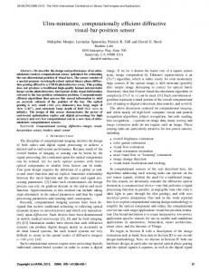
Fig. 1: Graph structure of pairwise comparametric image compositing. The HDR im(4) (1) (j>1) are age f1 is composited from the LDR source camera images f1...4 . Nodes fi rendered here by merely scaling and rounding the output from the comparametric camera response function (CCRF). To illustrate the details captured in the highlights and lowlights in the LDR medium of this paper, we include a spatiotonally mapped LDR (4) rendering of f1 .
we have N images, i ∈ {1, . . . , N }, and each image has exposure ki . The subscript indicates it is the i-th in a Wyckoff set[3], i.e. a set of images differing only in exposure, and by convention ki < ki+1 ∀ i < N . The notation f −1 means the mathematical inverse of f if it has only one argument, and otherwise means a joint estimator2 of photoquantity, q.
1.2. Mathematical Notation In this paper f as a function represents the camera response function (CRF), and as a scalar is a tonal value, and as a matrix is a tonal image (e.g. a picture from a camera). We consider a tonal value f to vary linearly with pixel value but on the unit interval, and given an n-bit pixel value v returned from a physical camera, we use fi = (v + 0.5)/2n , where 1 Often called radiance or luminance, though actually neither since the spectral response of cameras is not flat nor the same as the human eye.
978-1-4673-0046-9/12/$26.00 ©2012 IEEE
913
1.3. Prior work Robertson et al. state, “The first report of digitally combining multiple pictures of the same scene to improve dynamic range appears to be Mann[1]”[8]. In this section, we review this approach, which is also the most popular framework in prior work[7][8]. Estimates qˆi (x) ∈ R≥0 of the photoquantity q at 2 “Joint estimator” is used here in the sense that each photoquantity estimate depends simultaneously on multiple measurements.
ICASSP 2012
Input images
CCRF
(1)
(1)
f1
Output image
(1)
f2
(1)
f3
f4
(1)
f2
f (fΔ−1EV (f1, f2))
(2)
(1)
(1)
f1 = f (fΔ−1EV (f1 , f2 ))
f2
(2)
(2)
f1
f2
(1)
f1
2ΔEV
f1
(3)
f1
Spatiotonal mapping
Fig. 2: CCRF-based compositing of a single pixel. The floating-point tonal values f1 −1 and f2 are the arguments to the CCRF f ◦ fΔ which returns a refined estimate of an EV ideal camera response to the scene being photographed. This virtual camera’s exposure setting is equal to the exposure of the lower-exposure image f1 .
each spatial location x = (x, y) are determined independently from each input LDR image. Note that omitting x indicates the entire spatial domain. Camera output is given as fi = f (ki q + nqi ) + nfi where nqi and nfi are quantigraphic and imaging noise processes. Estimating photoquantity q requires knowledge of f −1 , so that qˆi = f −1 (fi )/ki . These estimates qˆi are then combined using a weighted sum to produce a single estimate qˆ of the photoquantity present in the original scene. 2. PROPOSED COMPOSITING METHOD 2.1. Compositing as Joint Estimation Our approach for creating an HDR image from N input LDR images begins with constructing a notional N -dimensional inverse CRF. We could then estimate photoquantity qˆ by writing qˆ = f −1 (f1 , f2 , ..., fN )/k1 , where f −1 is a joint estimator that may be implemented as an N -dimensional lookup table (LUT). Recognizing the impracticality of this for large N , we now consider pairwise recursive estimation. 2.2. Pairwise Estimation Assume we have N LDR images that are a constant change in exposure value apart, so that ΔEV = log2 ki+1 − log2 ki is a positive constant ∀ i ∈ {1, . . . , N − 1}. Now consider the case N = 2, with exposures k1 = 1 (without loss of generality, since exposures only have meaning in proportion to one another), and k2 = k. Then our estimate of the photoquan−1 (f1 , f2 ), where ΔEV = log2 k. To apply this tity is qˆ = fΔ EV pairwise estimator to N = 3 input images, we can write f (ˆ q) =
−1 −1 −1 f (fΔ (f (fΔ (f1 , f2 )), f (fΔ (f2 , f3 )))). EV EV EV
In this expression, we first estimate the photoquantity q based on images 1 and 2, and then again based on images 2 and 3, then these are combined, using the same joint estimator.
914
Fig. 3: An alternative graph structure for pairwise comparametric image compositing.
This pairwise estimation process may be expanded to any number N of input LDR images, using the recursive relation (j+1)
fi
(j)
(j)
−1 = f (fΔ (fi , fi+1 )), EV
where j = 1, . . ., N − 1, and i = 1, . . ., N − j. The final (N ) (1) output image is f (ˆ q ) = f1 , and in the base case, fi is the i-th input image. This recursive process may be understood graphically as in Fig. 1. This process forms a graph with estimates of photoquantities as the nodes, and comparametric mappings between the nodes as the edges. Rather than storing values of f −1 (f1 , f2 ), we instead store f (f −1 (f1 , f2 )) for runtime efficiency. We call this a comparametric camera response function (CCRF), since it always has the domain of a comparagram and range of a camera response function. A single estimation step using a CCRF is illustrated in Fig. 2. We use the same CCRF throughout, since f ◦ f −1 returns an exposure that is at the same exposure value as the less-exposed of the two input images (recall that we set k1 = 1), so the ΔEV between images remains constant at each subsequent level. All lookups per level can be performed in parallel, and N (N − 1)/2 recursive lookups are used in total. 2.3. Alternative graph topology Other connection topologies are possible, for example in the case N = 4, we can trade memory usage for speed by compositing using the form −1 −1 −1 f (ˆ q ) = f (f2Δ (f (fΔ (f1 , f2 )), f (fΔ (f3 , f4 )))), EV EV EV
in which case we only perform 3 lookups at runtime, instead of 6 using the previous structure. However, we must store −1 twice as much lookup information in memory: for f ◦ fΔ EV −1 as before, and for f ◦ f2ΔEV , since the results of the inner expressions are no longer ΔEV apart, but instead are twice as far apart in exposure value, 2ΔEV, as shown in Fig. 3.
������� ������� ��������� ���� ���� ���� ����
f4 = f (k4q)
ΔEV = 9
f1 = f (k1q)
f1 = f (k1q)
f1 = f (k1q)
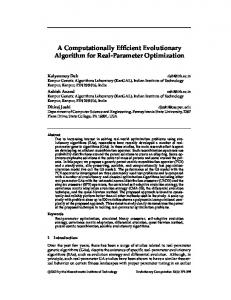
Fig. 4: Comparametric model fitting. Preferred saturation model parameters were found via non-linear optimization, using the method of least-squares with the Levenberg–Marquardt algorithm. The optimal comparametric model function, determined per color channel, is plotted directly on empirical comparasums to verify a good fit. Comparasums are sums of comparagrams from the same sensor with the same difference in exposure value ΔEV. They are shown range compressed using the log function, and color inverted, to show finer variation. Best results for comparametric compositing are found when the camera response function model parameters are optimized against a range of k values. Here k1 = 1 and k2 = 8, k3 = 64, k4 = 512 which implies that for comparametric image compositing we would use ΔEV = 3.
As a recursive relation for N = 2n , n ∈ N we have (j+1) fi
=
��� � ��� �
����
ΔEV = 6 f3 = f (k3q)
f2 = f (k2q)
ΔEV = 3
���
���
��� ��� ����� ����� � ��� �
���
���
Fig. 5: Trace plot of estimated standard deviations from a comparagram. Each estimate is proportional to the inter-quartile range (IQR), calculated from each column f1 and row f2 of a comparagram; here using ΔEV = 3 as given in Fig. 4. Gaussian smoothing is applied to reduce discontinuities due to edge effects, quantization, and other noise.
3.1. Probabilistic Model for CCRF
(j) (j) −1 f (fjΔ (f2i−1 , f2i )), EV
where j = 1, . . ., log2 N, and i = 1, . . ., N/2j−1 . The final (log N +1) (1) , and fi is the i-th input output image is f (ˆ q ) = f1 2 image. This form requires N −1 lookups. In general, by combining this approach with the previous graph structure it can be seen that comparametric image composition can always be done in O(N ) lookups ∀ N ∈ N.
Let scalars f1 and f2 form a Wyckoff set, and let random variables Xi = fi − f (ki q), i ∈ {1, 2} be the difference between observation and model, where k1 = 1 and k2 = k. The probability of qˆ, given f1 and f2 , is then P (q)P (f1 |q)P (f2 |q) P (f1 , f2 ) P (q)P (f1 |q)P (f2 |q) = �∞ P (f1 |q)P (f2 |q) dq 0
P (q = qˆ|f1 , f2 ) =
2.4. Constructing a CCRF lookup table To create a CCRF f ◦ f −1 (f1 , f2 , ..., fN ), the ingredients required are a camera response function f (q), and a method to estimate qˆ by combining multiple measurements. Then f ◦ f −1 is the camera response evaluated at the output of the joint estimator, and is a function of 2 or more tonal inputs fi . To create a LUT means sampling through the possible tonal values, so for example, to create a 1024×1024 LUT we could execute our qˆ estimation algorithm for all combi1 2 , 1023 , . . . , 1} and store the result nations of f1 , f2 ∈ {0, 1023 of f (ˆ q ) in a matrix indexed by [1023f1 , 1023f2 ], assuming zero-based array indexing. Intermediate values may be estimated using linear or other interpolation. 2.5. Incremental Updates In the common situation that there is a single camera capturing images in sequence, it is easy to perform updates of the final composited image incrementally, using partial updates, by only updating the buffers dependent on the new input.
∝ P (q = qˆ)P (f1 |q)P (f2 |q). For simplicity, we choose a uniform prior, which gives us Pprior (q = qˆ) = CONSTANT. Assuming zero-mean Gaussian noise, from Xi we have 2 ) Pmodel (fi |q) = Normal(μXi = 0, σX i � � 1 (fi − f (ki q))2 =√ exp − . 2 2σX 2πσXi i
We use the “preferred saturation”[4] model for f (q), as in 2 can be estimated from the interFig. 4. The variances σX i quartile range (IQR) along each column and row of the comparagram, i.e. using the “fatness” of the comparagram. A robust statistical formula, based on the quartiles of the normal distribution, gives σ ˆ ≈ IQR/1.349, as shown in Fig. 5. To maximize P (q = qˆ|f1 , f2 ) with respect to q, we remove constant factors and equivalently minimize −log(P ). Then the optimal value of q, given f1 and f2 , is �
3. EXAMPLE JOINT ESTIMATOR
qˆ = argmin q
In this section we describe a simple joint photoquantity estimator, using non-linear optimization to compute a CCRF. Examples of the results of this estimator are in Figs. 1 and 3.
915
� (f1 − f (q))2 (f2 − f (kq))2 + . 2 2 σX σX 1 2
In practice good estimates of optimal q values can be found using, for example, the Levenberg–Marquardt algorithm.
4. RESULTS AND DISCUSSION
Method
4.1. Implementation
Platform
We have implemented the proposed methods in Sections 2 and 3 in the C++ programming language for CPU code. We also implemented the method of Section 2 on a GPU (Graphics Processing Unit). The performance results are in Table 1. In Figs. 1, 2 and 3, the image compositing and photoquantity estimation were performed using the methods of Sections 2 and 3, with a pre-processing step of dark-frame subtraction. The camera images used were taken using a Flea3 CCD FireWire Video Camera from Point Grey Research, Inc. of Richmond, BC, Canada. The time required to construct 6 of the 1024×1024 CCRF LUTs for 3 color channels and 2 different ΔEV values using the algorithm of Section 3 was 20 sec., using an Intel 3.2GHz i7-970 CPU with Linux 2.6 running multithreaded code. The red CCRF for ΔEV = 3, resulting from the algorithm of Section 3, is shown in Fig. 2.
CPU (serial) CPU (threaded) GPU
4.2. Discussion Using direct computation for iterative methods is not feasible for realtime HDR video. For our simplistic probabilistic model given in Section 3, it takes over a minute (∼65 sec.) to compute each output frame using a single processor. Using the proposed method of Section 2, the multicore speedup is over 2500× for CPU-based computation, and 3800× for GPU-based computation (versus CPU), as shown in Table 1. Since GPUs implement floating-point texture lookup with linear interpolation in hardware, and can execute highly parallelized code, our method would seem to be a natural application of GPGPU (General Purpose Graphics Processing Unit) computation[9]. However, much of the time is spent waiting for data transfer between host and GPU; incremental updates are useful in this context, because we can re-use data and results from previous estimates, only transferring new data. The selection of the size of the LUT depends on the range of exposures for which it is used. It was found empirically that 1024×1024 samples of a CCRF is enough for the dynamic range of our setup. Further increases in the size of the LUT made no noticable improvement in output video quality. 5. CONCLUSION We have proposed a novel computational method for using multidimensional lookup tables, recursively if necessary, to estimate HDR output from LDR inputs. The runtime cost is fixed, irrespective of the algorithm implemented, if it can be expressed as a comparametric lookup. Pairwise estimation decouples the specific compositing algorithm from runtime, enabling a flexible architecture for realtime applications. We demonstrate a speedup of three orders of magnitude for nonlinear optimization based photoquantity estimation.
916
Direct Calculation
CCRF, Full Update
CCRF, Incremental
Speed in output Frames Per Second (FPS) 0.0154 0.103 –
51 191 272
78 265 398
Speedup 5065× 2573× –
Table 1: Performance of pairwise composition versus direct calculation of composite HDR image on 4 input LDR images of 640×480 pixels each. The CPU used is an Intel 3.2GHz i7-970, and the GPU is an NVIDIA GTX 460. Six 1024×1024 CCRFs were used, one per color channel per ΔEV. Since our Flea3 camera delivers a maximum of 120FPS, the rate was extended by presenting the same images 10× to each algorithm, doing a full copy each time to negate caching effects. The direct calculation performed simultaneous optimization on 4 inputs, however the resulting images were not observed to be significantly different than pairwise estimation in our experiments.
6. REFERENCES [1] S. Mann, “Compositing multiple pictures of the same scene,” in Proceedings of the 46th Annual IS&T Conference, Cambridge, Massachusetts, May 9-14 1993, The Society of Imaging Science and Technology, pp. 50–52, ISBN: 0-89208-171-6. [2] S. Mann and R.W. Picard, “Being ‘undigital’ with digital cameras: Extending dynamic range by combining differently exposed pictures,” in Proc. IS&T’s 48th annual conference, Washington, D.C., 1995, pp. 422–428. [3] S. Mann, “Comparametric equations with practical applications in quantigraphic image processing,” IEEE Trans. Image Proc., vol. 9, no. 8, pp. 1389–1406, August 2000, ISSN 1057-7149. [4] S. Mann, Intelligent Image Processing, John Wiley and Sons, November 2 2001, ISBN: 0-471-40637-6. [5] Chris Pal, Richard Szeliski, Matthew Uyttendaele, and Nebojsa Jojic, “Probability models for high dynamic range imaging,” in CVPR. 2004, pp. 173–180, IEEE. [6] Sing Bing Kang, Matthew Uyttendaele, Simon Winder, and Richard Szeliski, “High dynamic range video,” in ACM SIGGRAPH 2003 Papers, New York, NY, USA, 2003, SIGGRAPH ’03, pp. 319–325, ACM. [7] Miguel Granados, Boris Ajdin, Michael Wand, Christian Theobalt, Hans-Peter Seidel, and Hendrik P. A. Lensch, “Optimal hdr reconstruction with linear digital cameras,” in CVPR. 2010, pp. 215–222, IEEE. [8] Mark A. Robertson, Sean Borman, and Robert L. Stevenson, “Estimation-theoretic approach to dynamic range enhancement using multiple exposures,” Journal of Electronic Imaging, vol. 12, no. 2, pp. 219–228, 2003. [9] J. Fung, F. Tang, and S. Mann, “Mediated reality using computer graphics hardware for computer vision,” in Proc. Intl. Symp. on Wearable Computing ’02, 2002, ISWC 2002, pp. 83—89.