trajectory optimization, and mass properties analyses ... Collaborative optimization (CO) appears to be an ... Engine Simulation) is a web-based rocket engine.
Comparison of Collaborative Optimization to Conventional Design Techniques for a Conceptual RLV Timothy A. Cormier†, Andrew Scott†, Laura A. Ledsinger†, David J. McCormick† , David W. Way†, John R. Olds* Space Systems Design Laboratory School of Aerospace Engineering Georgia Institute of Technology, Atlanta, GA 30332-0150
Collaborative optimization (CO) appears to be an attractive multidisciplinary design optimization approach to solving this problem. Initial implementation attempts using CO have exhibited noisy gradients and other numerical problems. Work to overcome these issues is currently in progress.
ABSTRACT Initial results are reported from an ongoing investigation into optimization techniques applicable to multidisciplinary reusable launch vehicle (RLV) design. The test problem chosen for investigation is neither particularly large in scale nor complex in implementation. However, it does have a number of characteristics relevant to more general problems from this class including 1) the use of legacy analysis codes as contributing analyses and 2) non-hierarchical variable coupling between disciplines. Propulsion, trajectory optimization, and mass properties analyses are included in the RLV problem formulation. A commercial design framework is used to assist data exchange and legacy code integration.
NOMENCLATURE At Engine Throat Area (in2) Ae Engine Exit Area (in2) ACC Advanced Carbon-Carbon CA Contributing Analysis Cf Thrust coefficient (T/PcAt) CCD Central Composite Design CO Collaborative Optimization DSM Design Structure Matrix IO Iterative Optimizers Isp,vac Engine Vacuum Specific Impulse (sec) MER Mass Estimating Relationship MR Mass ratio (gross weight/burnout weight) Pc Engine Chamber Pressure (psia) r Engine mixture ratio RLV Reusable Launch Vehicle RSE Response Surface Equation RSM Response Surface Method Sref Wing Planform Area (ft2) SQP Sequential Quadratic Programming SSTO Single-Stage-to-Orbit Tvac Engine Vacuum Thrust (lbf) Tsl Engine sea-level Thrust (lbf) Tsl/We Engine sea-level thrust-to-weight ratio Tsl/Wg Vehicle sea-level thrust-to-weight ratio TABI Tailorable Advanced Blanket Insulation TUFI Toughened Uniform Fibrous Insulation Wdry Vehicle dry weight (lb) Wg Vehicle gross weight (lb) ∆V Velocity increment (ft/sec) ε Nozzle expansion ratio
The need for a formal multidisciplinary design optimization approach is introduced by first investigating two more conventional approaches to solving the sample problem. A rather naive approach using iterative sublevel optimizations is clearly shown to produce non-optimal results for the overall RLV. The second approach using a system-level response surface equation (RSE) constructed from a small number of RLV point designs is shown to produce better results when the independent variables are judiciously chosen. However, the response surface method (RSM) approach cannot produce a truly optimum solution due to the presence of uncoordinated sublevel optimizers in the three contributing analyses.
† - Graduate Research Assistant, School of Aerospace Engineering, Student member AIAA. * - Assistant Professor, School of Aerospace Engineering, Senior member AIAA. Copyright © 2000 by Timothy A. Cormier and John R. Olds. Published by the American Institute of Aeronautics and Astronautics, Inc. with permission.
1
SCORES may be run from the web or interactively from the UNIX operating system. For the purposes of this exercise, the UNIX version of SCORES was coupled with Phoenix Integration’s Model Center computational framework [2].
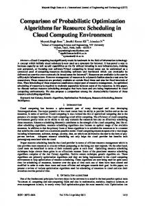
DESIGN PROBLEM STATEMENT The RLV to be designed is a second-generation SSTO vehicle that is launched from the Kennedy Space Center to the International Space Station (target orbit is 220 nmi x 220 nmi x 51.6º). The propulsion system is to be comprised of five high thrust-to-weight engines. Primary orbit insertion occurs at a transfer orbit of 50 nmi x 100 nmi x 51.6º. An on-orbit DV of 1100 fps is included to transfer the vehicle to the final orbit, rendezvous with the space station, and deorbit. The unpiloted vehicle is required to carry a 25,000 lb payload to orbit. The vehicle is also classified as a Generation 2 reusable launch vehicle, therefore all technologies are commensurate with 2005 technology freeze date for the first flight in 2010. The propellant tanks are to be made of an aluminum-lithium alloy. Graphite-epoxy is used in the exposed wing and carry through structure, as well as the primary, secondary, and payload structures. The thermal protection system uses ACC, TUFI tiles and TABI blankets. A schematic of the reference RLV is shown in Figure 1.
SCORES models a rocket engine in two parts. First, the chemical processes occurring in the combustion chamber are analyzed. Second, the expansion of hot gases in a convergent-divergent bell shaped nozzle is analyzed. The combustion process is assumed to occur adiabatically and at constant pressure. Additionally, all of the molecular species involved in the combustion are assumed to be thermally perfect gases. Finally, the initial velocity of the reactants is taken to be zero, thus assuming an infinite-area combustor. Therefore, the temperature and pressure in the combustion chamber are taken to be total values. The initial temperature of all the reactants is assumed to be 500K. The composition of the product gases is then determined through chemical equilibrium calculations. For the convergent-divergent nozzle, the flow is assumed frozen at the equilibrium conditions calculated for the combustion chamber. The expansion process is then modeled as a steady, inviscid, quasi1D, isentropic flow. Because of the quasi-1D assumption, cross-sectional area and expansion ratio are the only geometry variables. A detailed description of the nozzle contour is not necessary. The combustion products are assumed to be a mixture of calorically perfect gasses.
Figure 1. Schematic reference RLV
Thrust and Isp are calculated from the determined nozzle exit conditions. These estimates typically overpredict the thrust and Isp. This over-prediction is due to the ideal nature of the assumptions. Statistical performance efficiencies derived from existing flight hardware are then used to simulate losses by correcting downwardly adjusting the ideal thrust and Isp values.
DESIGN TOOLS PROPULSION SCORES (SpaceCraft Object-oriented Rocket Engine Simulation) is a web-based rocket engine analysis tool developed at Georgia Tech [1]. This tool suitable for use in conceptual design provides propulsion metrics such as thrust and specific impulse. Only top-level propulsion parameters are required for input. These parameters include mixture ratio, chamber pressure, throat area, and expansion ratio. The SCORES web-based tool is public and can be accessed at the Uniform Resource Locator (URL) address listed below:
SCORES provides an option to sizing the nozzle throat area to match a required thrust. Because the thrust is linear with throat area, the required throat area is simply the guessed value, 1 sq.in. by default, multiplied by the ratio of required thrust to calculated thrust. Therefore, no iteration is required, making the sizing option just as rapid as the analysis option. A low-fidelity estimation of thrust-to-weight (T/W) is also provided. This estimation is based on the premise that the engine will develop a constant power-toweight (P/W), where power, defined in Equation 1, is based on the chamber and exit enthalpies.
http://titan.cad.gatech.edu/~dwway/SCORES
2
· P = m(hc - he)
Primary booster structural materials include aluminum lithium alloy for the propellant tanks and graphite-epoxy composite for other structure such as exposed wings, the wing carry through, and verticals. Other subsystem highlights include an autonomous flight control system, electromechanical actuators, high power density fuel cells, lightweight avionics, and environmentally safe LOX-ethanol orbital maneuvering system (OMS) propellants.
(1)
Power is easily calculated within the same routines that predict thrust and Isp. If the P/W is known, then the T/W is found easily from the thrust and power by Equation 2. T /W = ( P/W )( T/P ) (2) To allow for differences in technology levels, SCORES provides a user input to select the T/W relative to other engines. The user may select “high”, “average”, or “low” from a pull-down menu. A selection of “average” uses a P/W of 0.017 MW/lb, while a selection of “high” or “low” uses a P/W of 0.023 or 0.015 MW/lb respectively.
The weights and sizing analysis provides a great deal information to the other analyses. Gross weight and wing reference area are given to the trajectory analysis and required sea_level static thrust is used by the propulsion analysis.
PERFORMANCE
COMPUTATIONAL FRAMEWORK
The tool used to simulate the trajectories of the RLV was the Program to Optimize Simulated Trajectories, POST [3]. POST is a Lockheed Martin and NASA code that is widely used for trajectory optimization problems in vehicle design. POST is a generalized event-oriented code that numerically integrates the equations of motion of a flight vehicle given definitions of aerodynamic coefficients, propulsion system characteristics, atmospheric tables, and gravitational models. Guidance algorithms used in each phase are user-defined. Numerical optimization is used to satisfy trajectory constraints and minimize a user-defined objective function by changing independent steering and propulsive variables along the flight path. POST runs in a batch execution mode and depends on an input file (or input deck) to define the initial trajectory, event structure, vehicle parameters, independent variables, constraints, and objective function.
In addition to the tools used for each discipline, a fourth tool, Phoenix Integration’s Model Center software package, was used to coordinate the system level analysis. Model Center a program that facilitates cross-platform analysis integration. For each of the disciplines, a wrapping script was written to properly direct the inputs and outputs of each tool. POST and SCORES were set up to run on UNIX workstations while the weights spreadsheet was run in Microsoft Excel on a Windows NT machine. Once each of the tools was properly wrapped and set up, one could easily link the inputs and outputs of the three disciplines to one another from within Model Center. These links were setup as appropriate to the design problem and the optimization method used to solve it. With the setup complete, Model Center is capable of transferring the appropriate information between the tools as well as coordinating their execution. Model Center also provides an optimization package, which was used in the methods that required system level optimization. This package is based on the popular optimization code, DOT [4]. For the collaborative optimization, sequential quadratic programming was used as the optimization algorithm. As system level optimization progresses, Model Center neatly records and organizes all the desired variables and constraints at each system level iteration. Model Center was also very helpful in the data collection for the RSM method by evaluating and collecting the results of multiple runs as setup by the user. All data collected by Model Center is easily exportable to Excel, making it easy to analyze the final results.
MASS PROPERTIES The weights and sizing analysis uses photographic scaling on a set of parametric mass estimating relationships (MER’s) that have a NASA Langley heritage. This analysis is performed using a Microsoft Excel spreadsheet. Using the results of the trajectory analysis, the vehicle is photographically scaled up or down until the available mass ratio on-board the currently sized vehicle (MRavail ) equal the required mass ratio from POST (MRreq). Since changing the vehicle scale changes the gross weight, sea-level thrust requirements, etc., the disciplines in the main iteration loop must be iterated until the vehicle size converges. This typically takes 4 to 5 iterations.
3
Without the use of a program like Model Center a great deal of user interaction is required to manually run each analysis. Manually running each analysis requires the user to change input variables, run the tool and collect the appropriate results. This process can be very time consuming and tedious. With so much interaction being required by the user to manually run each tool, there is also an increased likelihood of making mistakes. Though using Model Center certainly takes more time to set up, the cost of doing so is negligible when compared to the time savings and error reduction gained when doing the actual analysis. However, it should be mentioned that in using Model Center it was imperative that the disciplinary analyses be very robust. For disciplinary tools that traditionally require a bit a tweaking and interaction (such as POST), a little extra effort is required during setup to ensure that they perform consistently and accurately.
Table 1. Coupling variables in the conventional DSM Variable Tsl Tvac r Ae Isp,vac Tsl/We Sref Wg MR Wdry
Propulsion input output output output output output
Performance
Mass Properties
input input input input input output
input input input output output input output
RESPONSE SURFACE METHOD A central composite design (CCD) matrix was used to set the values of the global variables for the response surface method. Table 2 illustrates a generic CCD matrix.
Overall, the use of Model Center greatly increased the speed and efficiency with which the analyses were performed. In fact, with methods such as collaborative optimization that require many iterations and a great deal of computational time, it is difficult to imagine if manual implementation of such methods is even realistically feasible.
Table 2. Generic Central Composite Design Matrix
DESIGN METHODOLOGY The design structure matrix (DSM) is dependent upon the design method used. In conventional methods, variables are passed from one discipline to the others. A DSM for conventional methods is shown in Figure 2.
x1
x2
x3
-1 -1 -1 -1 1 1 1 1 0 −α α
-1 -1 1 1 -1 -1 1 1 0 0 0 −α α
-1 1 -1 1 -1 1 -1 1 0 0 0 0 0 −α α
0 0 0 0
Propulsion
Performance
0 0
Mass Properties
The results of the 15 runs of the array were used to fit a response surface to the design space. The constraints placed on the global variables were taken into account in the DOE by limiting the range of testing. The alpha values were set as the maximum range for the three design variables instead of the typical –1 and 1. The coded variables are shown in Table 3.
Figure 2. Conventional Method Design Structure Matrix The diagonal dotted lines indicate that local optimization occurs within a given contributing analysis (CA). A table depicting the flow of variables through each of the CA’s is shown in Table 1.
4
optimizer, which is configured to minimize a system level objective function under the constraint that the J terms of each discipline are kept below a certain tolerance. Each disciplinary tool is allowed to vary all of its usual inputs and local variables to minimize its own objective function. This allows for disciplinary experts to focus on their domain-specific issues while maintaining interdisciplinary compatibility. Table 4 summarizes the changes made for collaborative optimization while Figure 3 show the modified DSM.
Table 3. Response Surface Equation Coded Variables ε (x 1) r (x 2) T/W (x ) g
−α -1 0 1 α
30.00 38.11 50.00 61.89 70.00
4.500 5.615 7.250 8.885 10.000
3
1.20000 1.24054 1.30000 1.35946 1.40000
Once the response surface was determined, Matlab’s constrained function optimizer (a sequential quadratic programming based algorithm) was used to find the best design.
Table 4. Variable breakdown for Collaborative Optimization System Level Objective Function
COLLABORATIVE OPTIMIZATION
Variables
In collaborative optimization the general strategy is to obtain the optimal system configuration for a given objective function while allowing each CA to remain independent and still maintain interdisciplinary consistency. The primary benefit of collaborative optimization is that it allows the CA’s to maintain their discipline level optimization capabilities. Normally, this would present a problem as it is likely that the disciplinary objective functions are not consistent with the system level object function. For example, SCORES normally tries to maximize Isp, but this drives the engine weight up and may result in an engine configuration that does not lend itself to an optimal system level configuration.
Constraints
Minimize W dry: Tvac', r', ε', (T sl/We)', I sp', A e', Wg', MR' Jp