Progress In Electromagnetics Research M, Vol. 19, 61–75, 2011
COMPARISON OF CPML IMPLEMENTATIONS FOR THE GPU-ACCELERATED FDTD SOLVER J. I. Toivanen 1, * , T. P. Stefanski 2 , N. Kuster 2 , and N. Chavannes 3 1 Department
of Mathematical Information Technology, University of Jyv¨askyl¨a, P. O. Box 35, FI-40014 University of Jyv¨askyl¨ a, Finland 2 ETH
Z¨ urich, IT’IS Foundation, Z¨ urich, Switzerland
3 Schmid
& Partner Engineering AG (SPEAG), Z¨ urich, Switzerland
Abstract—Three distinctively different implementations of convolutional perfectly matched layer for the FDTD method on CUDA enabled graphics processing units are presented. All implementations store additional variables only inside the convolutional perfectly matched layers, and the computational speeds scale according to the thickness of these layers. The merits of the different approaches are discussed, and a comparison of computational performance is made using complex real-life benchmarks.
1. INTRODUCTION Recently, graphics processing units (GPUs) have become a source of computational power for the acceleration of scientific computing. GPUs provide enormous computational resources at a reasonable price, and are expected to continue their performance growth in the future. This makes GPUs a very attractive platform on which to run electromagnetic simulations. The FDTD method [1] in particular has been successfully accelerated on GPUs, showing excellent speedup in comparison to codes executed on central processing units (CPUs). Some early works reporting the use of GPUs for FDTD computations include [2], where a speedup factor of 7.71 over a CPU code was obtained in the case of a 2D simulation, and [3], where a successful implementation of a 3D code was reported. Received 10 June 2011, Accepted 27 June 2011, Scheduled 4 July 2011 * Corresponding author: Jukka I. Toivanen (
[email protected]).
62
Toivanen et al.
In 2006, NVIDIA released the compute unified device architecture (CUDA) parallel programming model, allowing for much simpler implementation of general purpose computations on GPUs manufactured by this company. Different implementation techniques and code optimization strategies for the FDTD method in CUDA are discussed in detail in [4–6]. Unfortunately, these works do not consider absorbing boundary conditions (ABCs), which are essential for the application of the FDTD method to the radiation and scattering problems in unbounded domains. Among the different possible ABCs, the convolutional perfectly matched layer (CPML) [7] is currently the state of the art, providing the best absorption properties and thus the most accurate simulation results. Although some studies on implementation of the CPML on GPUs also exist, they suffer from a lack of implementation details, and none show any kind of comparison of different implementation strategies. In [8], the CPML updates were implemented by extending the computation over the whole domain using zero update coefficients outside the PML regions. Using this approach, a speedup factor of 6.6 over a CPU code was reported. The drawback of such an approach is that the PML variables need to be stored over the whole domain, wasting a lot of memory resources. In [9, 10], CPMLs were implemented on a GPU in the case of a 2D FDTD code developed for radio coverage prediction purposes. The thickness of the PML was fixed to 16 cells to match the optimal size of CUDA thread blocks. This may not be a problem in the 2D case, but in the 3D case all added PML cells significantly increase the total number of cells in the simulation. In [11], performance of the standard YeeFDTD method with implemented CPMLs is reported for the sake of comparison to the FADI-FDTD GPU code. Although details of the implementation were not described, a speedup factor of 18.51 over a CPU code was reported. Unfortunately, the implementation suffers from low simulation throughput expressed in Mcells/s. GPU implementation of the FDTD method including CPML in the case of dispersive media is mentioned in [12], but implementation details are not given. Valcarce et al. [9] state that dividing the computation into several kernels for the different parts of the scenario is more suitable than having one single kernel computing the whole environment, because a single kernel would suffer from so called thread divergence. However, no actual comparison of these implementation strategies is presented. In this paper we show that the thread divergence is, in fact, not a big problem, and is actually more than compensated by the fact that some data can be reused and transactions to the slow global memory
Progress In Electromagnetics Research M, Vol. 19, 2011
63
are avoided. One of the features of PMLs is that the user has a simple way to make a trade-off between the accuracy and the computational burden by adjusting the number of PML cells. However, this is only possible if the implementation does not have a fixed number of PML cells, and the computational cost scales according to the number of cells. This is not necessarily the case for GPU implementations. In [13], for example, a shorter simulation time is actually reported in the case where the thickness of the PML is set to 16 cells instead of 10. Moreover, since the amount of memory available on the GPU is often the limiting factor for the simulation size, the PML implementation should only store variables inside the PMLs. In this paper we present three possible implementations of the CPML in CUDA, all of which have the abovementioned properties. The rest of this paper is organized as follows: Section 2 gives a short overview of programming in CUDA C, which is used in our GPU implementations; three different implementation strategies for the CPML are explained in detail in Section 3; Section 4 evaluates computational efficiency of the implementation strategies based on performance in complex real-life benchmarks; and finally, conclusions are drawn in Section 5. 2. CUDA PROGRAMMING MODEL CUDA enabled GPUs can be programmed using CUDA C, which is a subset of the C programming language with some extensions. In this framework, the pieces of code to be executed on the GPU are written as so called kernels. The kernels are executed in parallel by several threads in a single-instruction, multiple-data (SIMD) fashion. For devices of compute capability 2.0 or higher, concurrent kernels can also be launched, which represents a multiple-instructions, multipledata (MIMD) parallel model. In this contribution, we consider solely SIMD implementations of the CPML which run on larger number of available GPU devices. Contrary to CPU programming, CUDA threads are very lightweight, and a large number of threads is actually needed to obtain good multiprocessor occupancy and to hide memory access latency. The threads are divided into thread blocks, which can be one, two, or three-dimensional arrays. The threads within a block can be synchronized, and they can co-operate by exchanging data using fast shared memory. The number of threads in a block is limited, since all threads of a block are expected to reside on the same streaming multiprocessor and must share the limited resources of that
64
Toivanen et al.
processor [14]. Several thread blocks are executed in parallel on the different processors of the GPU. The thread blocks are logically organized into a one- or two-dimensional grid of blocks. The way in which the threads are organized into blocks (and grid of blocks) is called the execution configuration, and it can have a significant impact on the computational efficiency of the program. For instance, it affects the so called multiprocessor occupancy, which is the ratio between the number of active warps (groups of 32 threads) and the theoretical maximum amount of active warps on a multiprocessor. Each thread can have local variables stored into fast memory called registers. All threads can also read and write the global memory, but access to this memory has a very high latency. Parts of the global memory can also be bound to so called textures. Texture memory is cached, so that a read from the texture memory causes a read from the global memory only in a case of a cache miss. As Kim et al. [5] point out, the FDTD algorithm has a very low operational intensity, which is the amount of floating point operations per byte of data transferred from the global memory. Therefore, optimizing the arithmetic instructions or maximizing the multiprocessor occupancy are not very efficient means of optimizing the FDTD code. Instead, it is essential to minimize the number of transactions from the slow global memory by reusing data with the help of shared memory or registers. 3. IMPLEMENTATION DETAILS In this section, we present three different approaches to implementing CPML in CUDA. We shall, for brevity, look at the update of Ex component only. Handling of other E-field components, as well as all the H-field components, is completely analogous. In the FDTD method with CPMLs, the following update equation is used to compute the Ex component on time step n + 1/2: n+1/2
n−1/2
Ex |i+1/2,j,k = Ca |i+1/2,j,k Ex |i+1/2,j,k µ H |n n z i+1/2,j+1/2,k − Hz |i+1/2,j−1/2,k +Cb |i+1/2,j,k κyj ∆y ¶ n n Hy |i+1/2,j,k+1/2 −Hy |i+1/2,j,k−1/2 − +ΨEx,y |ni+1/2,j,k −ΨEx,z |ni+1/2,j,k . (1) κzk ∆z Similar equations can be written for other E- and H-field components (for details see [1]). Here Ca and Cb are the update coefficients
Progress In Electromagnetics Research M, Vol. 19, 2011
65
depending on the material in the cell and on the time-step size. This formulation is valid everywhere in the extended grid, including the PML regions. However, outside of the PML slabs ΨEx,y and ΨEx,z are zero, and the coordinate stretching variables κ are equal to one. The Ψ variables represent discrete convolution, and introduce the damping of the waves inside the PMLs. At each time step ΨEx,y is updated as follows: ΨEx,y |ni+1/2,j,k = byj ΨEx,y |n−1 i+1/2,j,k à ! Hz |ni+1/2,j+1/2,k − Hz |ni+1/2,j−1/2,k +cyj . (2) ∆y It is non-zero only inside PML slabs that terminate y-normal boundaries, and the update coefficients byj and cyj depend only on the distance from the PML interface in the boundary normal direction. Similarly, ΨEx,z is only non-zero inside z-normal PML slabs. In other words, two non-zero Ψ variables exist inside each PML slab, and where two or three PML slabs overlap, four or six Ψ variables exist, respectively. This is the potential source of the thread divergence in the update kernels, as the amount of work which has to be done varies depending on spatial location. The fraction of the CUDA code implementing the Ex update (1) without the Ψ variables is presented in Figure 1. Here sy and sz are regions of the shared memory where the Hy and Hz variables, respectively, have been loaded, ijk is the global index of this Ex component, matindx is the vector containing the material indices, shmidx is an index in the shared memory, and THREADSZ is the number of threads in a block in the z direction.
Figure 1. CUDA implementation of the Ex component update. Update of the Ey and Ez components is done in the same kernel, which enables us to reuse the H-field variables from the fast shared memory. Textures are used to fetch the update coefficients, as well as invdy and invdz containing 1/∆y and 1/∆z, respectively. The domain is divided between the threads so that each thread takes care of updating the E-field variables for single, fixed j and k,
66
Toivanen et al.
(0,0)
Z Y X
Figure 2. Arrangement of thread blocks.
Figure 3. CUDA computation of ΨEx,y in the combined updates approach. but for all i. That is, the kernel contains a for loop, which iterates through the domain in the x direction. This arrangement is illustrated in Figure 2, where the grey rectangles represent the thread blocks. The number of thread blocks depends on the domain size, and is usually much larger than in the figure. To obtain the halo for the updates, the thread blocks actually have an overlap so that some threads are only involved in loading the data, but not in performing the update. This is illustrated in Figure 2, where the E- and H-field halos related to thread block (1, 1) in the grid are shown. Size of the thread block in the figure is 16 × 16, and it updates 15 × 15 cells. Next we shall look at different possible approaches for implementing the CPML updates in the GPU-accelerated FDTD code. 3.1. Approach 1: Combined Updates First we consider an approach where the Ψ variables are updated by the same kernel as the respective E- or H-field. The benefit of this approach is clear: it enables maximal data reuse, as the E- and H-field values and the material parameters can be reused while performing the Ψ variable updates. The code performing the ΨEx,y update of Equation (2) is shown in Figure 3, where the data in the shared memory region sz appearing in the code of Figure 1 is reused, as well as the coefficient Cb. The update coefficients b and c are obtained using textures.
Progress In Electromagnetics Research M, Vol. 19, 2011
67
Not only do we avoid several loads from the global memory, but this approach also avoids some stores as the updated Ex component is written to the global memory only after the contributions of the Ψ variables are added. The drawback of this approach is the potential thread divergence: some of the threads in the block can update cells that are inside some PML slab, while some other threads may update cells that are not. The divergent threads are handled in hardware by the serialization of calculations, which can cause loss of performance in general. But in this case, when some threads update the Ψ variables, the threads related to cells that do not belong to the same PML slab are simply idle. Moreover, the PML update is a simple calculation taking only a very short time, after which the execution of the threads converges again [14]. 3.2. Approach 2: Single Kernel Updating All PML Regions We also wanted to test approaches where such thread divergence is minimal to see if any speedup would be gained. To this end, the domain was divided into PML regions so that each region consists solely of either one, two or three overlapping PML slabs (see Figure 4). If all six boundaries of the cubic domain are terminated by the PMLs, there are 3 × 3 × 3 − 1 = 26 of these regions. Each of the PML regions is then handled by one or more thread blocks, so that the threads are organized in the yz plane, and they iterate in the x direction. There are couple of difficulties related to this approach. Finding the index of the FDTD cell that a thread is updating is no longer trivial as the location of the corner of the region must be known. The indices
3
2
3
2
1
2
3
2
3
Figure 4. Division of the domain into regions. overlapping PML slabs is also indicated.
The number of
68
Toivanen et al.
of the region corners were therefore stored to texture memory, from which they were fetched by each thread to compute the cell index. Moreover, since we want to launch the thread blocks updating all the regions simultaneously, the kernel has to include conditionals to decide, for example, which Ψ variables need to be updated. However, thread divergence is still minimal despite this conditional execution because all threads in the same thread block update the same number of Ψ variables. 3.3. Approach 3: Specialized Kernel Updating Each PML Boundary The performance of Approach 2 was not as good as Approach 1 in computational tests (see next Section). Therefore we implemented one more approach, where the kernels do not include such conditional execution as Approach 2. Instead, a specialized kernel is launched for each of the boundaries, which means that each kernel updates exactly two Ψ variables. Execution configuration is as follows. Each thread is given an index in the boundary surface, and it iterates through the PML slab in the boundary normal direction. The update procedure is shown in Figure 5.
Figure 5. CUDA computation of ΨEx,y in the specialized kernels approach. To update each Ψ variable we need two H-field variables to compute the derivative in the boundary normal direction. Since the kernel also iterates in the boundary normal direction, one of those can be reused in the next step. There is no need to share these values between the threads and so the H-field variables are stored in registers (hz1 and hz0 in the code). One major issue to be considered when programming in CUDA is coalesced memory access. The minimum size of a memory transaction in the current CUDA enabled devices is 32 bytes [14]. Therefore, if the threads access 4 byte floating point variables in a scattered manner, a 32 byte transaction is issued for each variable, and the effective memory throughput is divided by 8. However, if we meet certain restrictions (which depend on the version of the CUDA enabled GPU device), several memory transactions performed by threads in
Progress In Electromagnetics Research M, Vol. 19, 2011
69
the same warp can be grouped together into so-called coalesced access. In general this means that threads with neighbouring indices should access neighbouring data in the global memory. Our E- and H-field data is organized in z-fastest order. As the threads are organized in yz and xz planes in the case of x-normal and y-normal boundaries respectively, the coalesced access is easy to achieve in these cases by simply assigning the cells to the threads in zfastest order. However, things become difficult in the case of z-normal boundary, as the threads should be organized in the xy plane. Because of the uncoalesced access, in initial tests measured performance was 7.6 times worse for the kernels updating PML slabs terminating z-normal boundaries compared to those updating x- or y-normal boundaries. The overall effect on code performance was devastating, even though the PML regions only corresponded to a relatively small portion of the computational domain. For this reason we decided to design a different type of kernel for the z-normal boundaries. We can exploit the fact that the PML also has a dimensionality in the z direction, and assign each thread block a piece of xy plane so that the size of the block exceeds the thickness of the PML. The threads then load the field variables into shared memory in a coalesced manner, and each thread then updates the Ψ variables using the data from the shared memory. The resulting arrangement of the thread blocks is shown in Figure 6.
Z
Y X
Figure 6. Arrangement of thread blocks for PML updates on xnormal, y-normal, and z-normal boundaries in specialized kernels approach (exploded view).
70
Toivanen et al.
Notice, that the different kernels update the same field values on the overlapping slabs. Therefore, the kernels cannot be launched in parallel even on devices with high enough compute capability, since this would result in a race condition. 4. NUMERICAL RESULTS Next we present the numerical results from benchmarks performed on a Tesla C1060 GPU having 30 streaming multiprocessors (240 CUDA cores) and 4 GB memory, and a computer having two dual core Opteron 2.4 GHz processors and 16 GB memory. Since all the described approaches implement the same update equations, the results are the same within single precision floating point accuracy. The methods were found to give the correct results when comparing against a commercially available solver, and we therefore look only at the speed of computations. We consider the effective simulation speed, so that the PML cells are not included in the cell count of the computational domain. We report the peak speed measured over 10 second intervals, which was found to be a fairly stable measure in the sense that results in different runs usually differ very little. 4.1. Example 1: Cubic Domain First we consider a simple test case to see what effect the size of the computational domain has on the simulation speed. We used a vacuum filled cubic domain of varying size with 10 cells thick CPML on all six boundaries of the domain. We also wanted to determine the optimal size of the thread blocks. Since the field variables are stored in the global memory in z-fastest order, a larger thread block size in the z direction can potentially reduce the number of memory transactions. On the other hand, a larger block size can increase the slowdown caused by thread divergence. Figure 7 shows the simulation speeds using the different approaches, i.e., (A1) combined updates, (A2) single kernel updating all PML regions, (A3) specialized kernel updating each PML boundary, and using a thread block size of 16 × 16 and 32 × 16. On small domains the smaller thread block size performs slightly better in all approaches, but the difference is not very significant. However, when the size of the domain is 2003 or larger, the larger thread block size performs significantly better. For this reason, the thread block size 32 × 16 was chosen for the rest of the presented examples.
Progress In Electromagnetics Research M, Vol. 19, 2011
71
Figure 7. Simulation speed as a function of the domain size for different PML implementations: (A1) combined updates, (A2) single kernel updating all PML regions, (A3) specialized kernel updating each PML boundary.
Figure 8. The full body model and the MRI head coil. 4.2. Example 2: MRI Coil As the second test case we consider the interaction of electromagnetic field with the human body. The model before voxeling is shown in Figure 8. As seen, the model includes a large number of different materials. Notice that as the head is the primary target of interest in such a simulation, PMLs could also be used to terminate the torso. In this case the whole torso was voxeled, but a more dense grid was used in the area containing the head. Harmonic excitation was introduced by 8 different edge sources positioned around the MRI coil. The size of the grid was 312 × 328 × 325, resulting in 33.4 × 10⁶ cells in the simulation. As the extraction of simulation results can greatly reduce simulation speeds, we monitored only one edge during this test. We compared the performance of the implementations when a variable number of PML cells was added to each of the six boundaries of the computational domain. The results are shown in the Figure 9. For comparison, the simulation speed using a GPU implementation of the first order Mur analytical ABC instead of PMLs was 500 Mcells/s. Speedup factors between 21.0 and 36.6 were observed when compared to a CPU implementation of the FDTD method with PMLs.
Toivanen et al.
Simulation speed (Mcells/s)
72
500 450 400 350 300
A1 A2 A3
446
446 391
400
385 352
373
367 322
349
318 282
250 200 150 100 50 0
4
8
12
16
PML thickness (cells)
Figure 9. Simulation speed in the MRI example for different PML implementations: (A1) combined updates, (A2) single kernel updating all PML regions, (A3) specialized kernel updating each PML boundary.
Figure 10. Magnitude of the magnetic field on the surface of the car. 4.3. Example 3: Car The next test case is a computation of the scattering of a plane wave from a car. The simulation grid was 519 × 239 × 159 ≈ 19.7 × 10⁶ cells. The voxeling of the car model can be seen in Figure 10, as well as the magnitude of the simulated magnetic field on the surface of the car. The simulation speeds using the different PML implementations for a variable number of PML cells are shown in Figure 11. Simulation speed using the Mur ABC was 287 Mcells/s, and speedup factors compared to the CPU implementation varied between 16.5 and 21.1.
Progress In Electromagnetics Research M, Vol. 19, 2011
Simulation speed (Mcells/s)
300 250
A1 A2 A3
278
265 246
246
242 222
242
238 212
200
73
208
195 174
150 100 50 0
4
8
12
16
PML thickness (cells)
Figure 11. Simulation speed in the car model example for different PML implementations: (A1) combined updates, (A2) single kernel updating all PML regions, (A3) specialized kernel updating each PML boundary. In general, the simulation speeds in this example were slower than in the previous examples, which was mostly caused by the plane wave excitation implemented as a set of separately updated edge sources. Moreover, the simulation domain is quite small in the z direction, which is not optimal in view of the previous results (see Figure 7). 5. CONCLUSIONS In this paper, we have presented details of three distinctively different implementations of CPML for the 3D FDTD method on CUDA enabled GPUs. Efficiency of the implementations was evaluated using complex real-life benchmarks. All the implementations have the following attractive properties: the additional variables needed for the CPML updates are stored only inside the PMLs, the number of PML cells can be chosen freely, and the computational cost scales according to the PML thickness. In Approach 1, updates of PML variables were performed in the same kernel with the respective E- or H-field update. Some thread divergence occurs if only some of the threads in a thread block update cells inside a PML. However, such divergence is not a big problem as the CPML updates include only very few floating point operations, and the execution of threads converges after the update. This approach also results in maximal reuse of the data loaded from the slow global memory. This is a big advantage as data transfer is the bottleneck in GPU computations with low arithmetic intensity algorithms such as the FDTD method. This approach turned out to be the most efficient
74
Toivanen et al.
in almost all cases. Approach 2 is based on dividing the domain into regions having a uniform number of overlapping PML slabs. The thread blocks performing the PML updates can be launched in parallel without the risk of a race condition, and thread divergence is minimal. However, the kernel is more complicated than in other approaches, and it turns out to be less efficient in all numerical benchmarks. Finally, in Approach 3 specialized kernels were launched separately for each of the six sides of the domain. The kernels have to launch sequentially to avoid a race condition because different kernels update the same field variables in regions where several PML slabs overlap. A drawback of this approach compared to Approach 1 is that less data can be reused. On the other hand, the kernels are now less complicated and use less registers compared to the previous approaches, which can lead to a possible increase in multiprocessor occupancy. Moreover, there is less thread divergence. The performance of this approach is generally slightly worse than Approach 1, even though it does perform slightly better in some cases (see Figure 11). In view of our findings, Approach 1 can be recommended as the way of implementing CPML in CUDA. The computational performance of this approach was generally better than the presented alternatives, and it is also the simplest one to implement. It is a topic of further study if a more efficient implementation could be created for the devices of compute capability 2.0 or higher (the Fermi generation GPUs), which support caching for the global memory, and are capable of launching different kernels concurrently. REFERENCES 1. Taflove, A. and S. C. Hagness, Computational Electrodynamics: The Finite-Difference Time-Domain Method, 3rd edition, Artech House, Norwood, 2005. 2. Krakiwsky, S. E., L. E. Turner, and M. M. Okoniewski, “Acceleration of finite-difference time-domain (FDTD) using graphics processor units (GPU),” 2004 IEEE MTT-S International Microwave Symposium Digest, Vol. 2, 1033–1036, 2004. 3. Humphrey, J. R., D. K. Price, J. P. Durbano, E. J. Kelmelis, and R. D. Martin, “High performance 2D and 3D FDTD solvers on GPUs,” Proceedings of the 10th WSEAS International Conference on Applied Mathematics, 547–550, World Scientific and Engineering Academy and Society (WSEAS), 2006. 4. Sypek, P., A. Dziekonski, and M. Mrozowski, “How to render
Progress In Electromagnetics Research M, Vol. 19, 2011
5.
6.
7.
8.
9.
10.
11.
12. 13.
14.
75
FDTD computations more effective using a graphics accelerator,” IEEE Transactions on Magnetics, Vol. 45, 1324–1327, 2009. Kim, K.-H., K. Kim, and Q.-H. Park, “Performance analysis and optimization of three-dimensional FDTD on GPU using roofline model,” Computer Physics Communications, Vol. 182, 1201–1207, 2011. Donno, D. D., A. Esposito, L. Tarricone, and L. Catarinucci, “Introduction to GPU computing and CUDA programming: A case study on FDTD [EM programmer’s notebook],” IEEE Antennas and Propagation Magazine, Vol. 52, 116–122, 2010. Roden, J. A. and S. D. Gedney, “Convolution PML (CPML): An efficient FDTD implementation of the CFS-PML for arbitrary media,” Microwave and Optical Technology Letters, Vol. 27, No. 5, 334–339, 2000. Inman, M. J., A. Z. Elsherbeni, J. Maloney, and B. Baker, “GPU based FDTD solver with CPML boundaries,” Proceedings of 2007 IEEE Antennas and Propagation Society International Symposium, 5255–5258, 2007. Valcarce, A., G. D. L. Roche, and J. Zhang, “A GPU approach to FDTD for radio coverage prediction,” Proceedings of 11th IEEE Singapore International Conference on Communication Systems, 1585–1590, 2008. Valcarce, A., G. de la Roche, A. J¨ uttner, D. L´opez-P´erez, and J. Zhang, “Applying FDTD to the coverage prediction of WiMAX femtocells,” EURASIP Journal on Wireless Communications and Networking, Vol. 2009, 2009. Tay, W. C., D. Y. Heh, and E. L. Tan, “GPU-accelerated fundamental ADI-FDTD with complex frequency shifted convolutional perfectly matched layer,” Progress In Electromagnetics Research M, Vol. 14, 177–192, 2010. Zunoubi, M. R. and J. Payne, “Analysis of 3-dimensional electromagnetic fields in dispersive media using CUDA,” Progress In Electromagnetics Research M, Vol. 16, 185–196, 2011. Mich´ea, D. and D. Komatitsch, “Accelerating a three-dimensional finite-difference wave propagation code using GPU graphics cards,” Geophysical Journal International, Vol. 182, No. 1, 389– 402, 2010. NVIDIA Corporation, “NVIDIA CUDA C programming guide,” Version 3.2, 2010.