Convolutional codes with Viterbi decoding are also compared ... low error rate given long codes. ... systems low bit error rate (BER) is a necessary but not a.
Comparison of LDPC Block and LDPC Convolutional Codes Based on their Decoding Latency Najeeb ul Hassan, Michael Lentmaier, and Gerhard P. Fettweis Vodafone Chair Mobile Communications Systems Dresden University of Technology (TU Dresden), 01062 Dresden, Germany Email: {najeeb.ul.hassan, michael.lentmaier, fettweis}@ifn.et.tu-dresden.de Abstract—We compare LDPC block and LDPC convolutional codes with respect to their decoding performance under low decoding latencies. Protograph based regular LDPC codes are considered with rather small lifting factors. LDPC block and convolutional codes are decoded using belief propagation. For LDPC convolutional codes, a sliding window decoder with different window sizes is applied to continuously decode the input symbols. We show the required Eb /N0 to achieve a bit error rate of 10−5 for the LDPC block and LDPC convolutional codes for the decoding latency of up to approximately 550 information bits. It has been observed that LDPC convolutional codes perform better than the block codes from which they are derived even at low latency. We demonstrate the trade off between complexity and performance in terms of lifting factor and window size for a fixed value of latency. Furthermore, the two codes are also compared in terms of their complexity as a function of Eb /N0 . Convolutional codes with Viterbi decoding are also compared with the two above mentioned codes.
I. I NTRODUCTION Shannon in his famous article in 1948: “A mathematical theory of communication” [1] has proved that a coded transmission with rates close to capacity is possible with arbitrarily low error rate given long codes. In practical communication systems low bit error rate (BER) is a necessary but not a sufficient requirement. Additionally, one needs to consider the latency caused by introducing channel coding. Convolutional codes have been considered as a good choice for applications with strong latency constraints [2], whereas LDPC block codes (LDPC-BCs) perform better than convolutional codes when the requirements on latency are rather permissive. An investigation in terms of decoding latency is carried out in [2], where convolutional codes and LDPC-BCs are compared under equal structural latency. In [3] stack sequential decoding [4] is applied to convolutional codes with large memory and the range of latencies over which convolutional codes are better than block codes is increased. In this paper, we consider the convolutional counter part of LDPC-BCs, termed as LDPC convolutional codes (LDPCCCs). It can be observed that the LDPC-CC ensembles have better belief propagation decoding thresholds than the block codes they are constructed from [5] [6] [7]. In this paper, we compare the performance of LDPC-BCs and LDPC-CCs over a range of latencies. While the pipeline decoder considered in [8] [9] is suitable for highly parallel high-speed processing
of LDPC-CCs, its structure results in fairly large decoding latency. In order to reduce the decoding latency, a sliding window decoder has been investigated in [10], which is a onesided variant of the window decoder introduced in [6] for a density evolution analysis. We compare the performance of such a suboptimal decoding scheme with LDPC-BCs under low latency over additive white Gaussian noise (AWGN) channel. For reference purpose, we also compare the two above mentioned codes with convolutional codes under Viterbi decoding [11]. The paper is organized as follows; Section II introduces the system model used throughout the paper to compare the codes on the basis of their decoding latency. Section III describes the considered codes together with their respective latency. Moreover, a simple yet effective stopping rule for the iterative process in LDPC-CCs is also introduced. A comparison in terms of performance and complexity is carried out for the codes under consideration in Section IV. Section V concludes the paper. II. S YSTEM M ODEL As shown in Fig. 1, we consider a digital transmission system to compare the latency introduced by different channel codes. The channel encoder maps an information block ut of k information bits to a codeword ct of length n with code of rate R = k/n. The coded bit stream is then mapped to xt ∈ {+1, −1} and transmitted over an AWGN channel. On the receiver side the noisy received word yt is passed to the channel decoder which removes the redundancy added ˆt of the by the channel encoder and produces the estimates u transmitted information bits ut . For a performance comparison of different codes the information bits and the estimates produced by the channel decoder are used to calculate the BER. Channel
ut Source
Channel Encoder
yt
xt
ct BPSK
+
noise
Fig. 1.
The system model
Channel Decoder
ˆt u BER
III. C ODES AND L ATENCY C ALCULATION A. Low-Density Parity-Check Block Codes A regular (J, K) LDPC-BC is characterized by a sparse parity-check matrix H, containing exactly J ones in each column and K ones in each row. Here we restrict ourselves to protograph based codes. A protograph is a rather small bipartite graph consisting of nc check nodes and nv variable nodes and is represented by its bi-adjacency matrix B, called base matrix. The matrix H of a particular code is obtained by using a copy-and-permute operation where each 1 in B is replaced by an N × N permutation matrix and each 0 by an N × N zero matrix. The resultant parity-check matrix consists of N nc check and N nv variable nodes. The permutation matrices can be generated using progressive edge growth (PEG) algorithm introduced in [12] such that short cycles are avoided, wherever possible. A regular LDPC-BC represented by a matrix H maps an input information word of length k = N (nv − nc ) to an output codeword of length n = N nv bits. Similarly, at the decoder side the entire frame needs to be received before belief propagation (BP) is applied. This causes a latency of N nv R information bits. So the structural decoding latency TB of a block code in terms of number of information bits is given as TB = N (nv − nc ).
(1)
1 We consider here the structural latency as it is a feature of the coding scheme itself, regardless of current and future ways of implementation. Hence, as pointed out in [2], it provides an ultimate lower bound on the actual delay of the code.
b
b
b
yt
yt+W
b
b
yt−m
m
W −1 yt+W −1
The encoder maps the input information word ut to the output codeword ct . In case of block coding the consecutive blocks are encoded independently of each other whereas, in conventional convolutional coding the encoding of ct depends on several input blocks ut , ut−1 , . . . ut−m , where m is the memory of the code. Often this mapping is done frame wise, which requires the full frame of length k information bits to be available at the input before the mapping can be started. Similarly, decoding cannot start before the complete frame of n code bits is available at the input of the decoder. The time that the en/decoder has to wait for the input bits before the mapping can take place is due to the structure of the code and hence termed as structural latency 1 . We consider here only the decoding latency since convolutional codes as compared to block codes have an advantage in terms of structural latency of the encoder. The input block length k for convolutional codes is usually in the order of a few information bits. Consider as an example a convolutional code of rate R = 1/2 with k = 1 and n = 2. The encoding can be performed as soon as 1 information bit is available at the input of the encoder. Whereas, in case of block codes k is the length of one frame which is usually large. Furthermore, the processing capability is considered to be infinite and hence processing latency due to the mapping operation in the encoder and the decoder is neglected. The transmission delay is not considered as its effect on all the codes is equal.
b
ˆt u
Decoding
Fig. 2.
Window decoder representation for latency calculation.
For a particular protograph the latency depends only on the lifting factor. Codes of various lengths can be constructed by using different lifting factors in the PEG algorithm. B. Low-Density Parity-Check Convolutional Codes Low-density parity-check convolutional codes are characterized by a semi-infinite diagonal type parity-check matrix H. Analogous to LDPC-BCs the parity-check matrix H of the LDPC-CCs can also be derived by the protograph expansion. Consider the transmission of a sequence of codewords ct , t = 1, . . . , L of length n each. In case of block encoding, these L codewords are encoded independently. Whereas, for LDPCCCs these L blocks are coupled over various time instants t. The memory m of the code determines the maximal distance between a pair of coupled blocks. Consider an example of a regular ensemble of a (J, K) block code defined by its base matrix B with dimension nc × nv where nc and nv are the number of check and variable nodes in the base protograph. The edges are spread according to the component base matrices B0 , B1 , . . . Bm such that the following condition holds [13], m X
Bi = B.
i=0
The resultant ensemble described by means of a matrix B0 .. . B[1,L] = Bm
of terminated LDPC-CCs can be convolutional protograph with base .. ..
. .
B0 .. . Bm
(2)
(L+m)nc ×Lnv
The parity-check matrix H of the LDPC-CC can be obtained by applying the lifting procedure to the base matrix in (2). In this paper we construct the parity-check matrix of an LDPCCC by unwrapping [8] the corresponding H matrix of an LDPC-BC. Window Decoding (WD): Due to the convolutional structure of the code, the variable nodes which are at least N (m + 1) units apart in the matrix H are not connected to the same
check node. This characteristics is exploited in the window decoder to decode the terminated LDPC-CC continuously [10]. The sliding window decoder of size W operates on a section of W · N nc rows and W · N nv columns of the matrix H. This corresponds to W coupled blocks of size N nv code bits each. Moreover, due to the memory of the code the WD also requires read access to the m previously decoded blocks as shown in Fig. 2. The size W of the window can range from m + 1 to L − 1. At every window position t only the first N nv symbols at time instant t are decoded and hence termed as target symbols. After a certain number of iterations It are performed at position t, the window slides N nc rows down and N nv columns right in H. Figure 2 shows the symbols inside the window when symbols in yt are the target symbols. The decoding of yt can only start once the succeeding W − 1 received words are available. The structural latency for the window decoder TWD in terms of number of information bits can be expressed as [14] TWD = W · N nv · R.
(3)
The decoding latency of a window decoder depends on W and N . One can either use a strong code by using a large lifting factor together with a small value for W or a weak code (small N ) can be decoded using a relatively large window size W . In the next section the choice of N and W is analyzed in detail. Stopping Rule: We introduce a simple, yet effective stopping rule based on the estimates of BER using the log likelihood ratios (LLR) of the target symbols within a window. The BER is estimated for the target symbols of current window and the window moves forward only when the estimated BER is less than the target BER or the maximum number of iterations are performed. We call this soft BER estimate as it is calculated using the soft values of the coded bits. The soft BER is calculated as follows. The probability that the hard decision of the ith bit, having LLR Li , is wrong can be given as 1 1 + e|Li | This is termed as soft bit error indicator in [15]. Once the soft bit error indicators for all the target symbols in a window are available, the estimated BER Pˆb can be calculated as the expected value of Z, Zi =
Pˆb = E[Z] =
Nn 1 Xv Zi . N nv i=1
(4)
The window moves forward only when Pˆb is less than the target BER or the maximum number of iterations It,max within a window at time instant t is reached.
applied to continuously decode the input bit stream. Branch metrics are computed after receiving the k information bits corresponding to one trellis segment. The maximum likelihood path is chosen after receiving τ trellis segments. The Viterbi decoder can be represented in the same way as WD in Fig. 2 with W = τ . Hence, the structural latency of the Viterbi decoder TV in terms of number of information bits is given as TV = kτ.
(5)
IV. S IMULATION R ESULTS The codes described in the previous section are compared under different latency values. The system model in Fig. 1 is used for the comparison and the Eb /N0 required to achieve a BER of 10−5 is measured for the codes under consideration. Without loss of generality, we restrict ourselves to protograph based regular LDPC-BCs and LDPC-CCs. Moreover, a comparison between LDPC-BCs and LDPC-CCs on the basis of effective number of updates per variable node is also presented. A. Performance Comparison Table I shows the base matrix B and the corresponding component matrices, used in edge spreading, for rate R = 1/2 LDPC-BCs and LDPC-CCs. In case of window decoding the edge spreading is chosen such that B0 contains multiple edges to avoid the low degree variable nodes at the right end of window. Such an ensemble has been proposed in [10] to achieve the target BER with a smaller W . The maximum number of iterations are set to Imax = 500 for LDPC-BCs and the iterative process terminates as soon as all the checks are satisfied. Whereas, in WD the maximum number of iterations per window at time t is fixed to It,max = 500 and the soft BER estimate in (4) with target BER of 10−6 is used as a criterion to shift the window to a new position. In case of LDPC-BCs the decoding latency in (1) depends only on the lifting factor used in the construction of the code. In case of LDPC-CC the decoding latency TWD depends on the lifting factor N and on the choice of the window size W . Consider a latency of TWD = 200 information bits. Figure 3 shows BER curves for WD when lifting factors of N = 25 and N = 40 with W = 8 and W = 5 are used, respectively. The BER curve for a (4, 8) LDPC-BC using N = 50 is also plotted. LDPC-CCs with both choices perform better than LDPC-BC, but using N = 40 with W = 5 results in better TABLE I C OMPONENT M ATRICES USED IN THE E DGE S PREADING OF LDPC-BC S AND LDPC-CC S . Code
B
m
Bi
C. Convolutional Code
LDPC-BC
[3 3]
2
B0,1,2 = [1 1]
A continuous encoding for a rate R = k/n convolutional code can be realized by a simple circuit based on shift registers with ν memory elements. Similarly, Viterbi decoding can be
LDPC-BC
[4 4]
3
B0,1,2,3 = [1 1]
LDPC-CC
[4 4]
2
B0 = [2 2], B1,2 = [1 1]
0
6
10
LDPC-BC, N=50 LDPC-CC, N=25, W=8 LDPC-CC, N=40, W=5
-1
Viterbi, ν = 10 (3,6) LDPC-BC (4,8) LDPC-BC (4,8) LDPC-CC
5.5
10
5
Bit Error Rate
-3
10
-4
10
4.5 4 3.5
W
Required Eb/N0 in dB
-2
10
3 N=25 -5
10
2.5
-6
10 1
1.5
2
2.5 Eb/N0 in dB
3
3.5
4
Fig. 3. BER for (4, 8) LDPC-BCs and LDPC-CCs with a decoding latency of 200 information bits.
2
100
N=60 200 300 400 Decoding latency in information bits
500
Fig. 5. Required Eb /N0 to achieve Pb = 10−5 for (3, 6) and (4, 8) LDPC-BCs and (4, 8) LDPC-CCs.
4.5 N = 25, W = 3,...,8 N = 40, W = 3,...,8 N = 60, W = 4,...,6
4.25
Required Eb/N0 in dB
4 3.75 3.5 3.25 3 2.75 2.5 50
100
200 300 150 250 Decoding latency in information bits
350
400
Fig. 4. Required Eb /N0 for (4, 8) LDPC-CCs with N = 25, 40 and 60 with different window sizes.
performance. The same is observed in [13] Fig. 10, when the gain between LDPC-BC and LDPC-CC decreases by using a window size of W = 12 with N = 250 as compared to W = 6 and N = 500. Moreover, for a particular code (fixed N ), performance improves by increasing W but eventually the rate of this improvement decreases. Figure 4 shows the required Eb /N0 to achieve a BER of 10−5 when N = 25, 40 and 60 is used with different values of W . After a certain point using a higher lifting factor together with a rather small window size gives better performance. But the window size can be adjusted in the decoder depending on the requirements of the application at the given time without changing the encoder. This provides a flexibility in terms of latency and performance of the code as shown in Fig. 5 for N = 25 and N = 60. In order to compare over the range of latencies, curves similar to Fig. 3 are generated for different values of N and W and the best combination in terms of required Eb /N0 at a BER of 10−5 is chosen. Figure 5 shows the required Eb /N0 to achieve Pb = 10−5 for the codes under discussion.
The horizontal axis represents the decoding latency TV , TB and TWD for convolutional codes, LDPC-BCs and LDPC-CCs respectively. In case of Viterbi decoding a rate R = 1/2 convolutional code with ν = 10 and different values of τ is used. For Eb /N0 = 3.1 dB, the Viterbi decoder needs a minimum latency of TV = 80 information bits and a (4, 8) LDPC-BC requires a latency of TB = 380 information bits to achieve Pb = 10−5 . This gap can be reduced by ≈ 100 information bits by using a (4, 8) LDPC-CC. Also a (3, 6) LDPC-BC performs better than a (4, 8) LDPC-BC because of the lower block code threshold. Furthermore, for all the range of latencies, the (4, 8) LDPC-CC outperforms the (3, 6) and (4, 8) LDPC-BC. B. Complexity Comparison For complexity analysis between LDPC-BCs and LDPCCCs, we compare the average number of updates required per variable node. In case of LDPC-BC the updates per node are equal to the number of iterations performed before the correct codeword is obtained. Due to the sliding window decoder for LDPC-CCs, each variable node is updated in multiple window positions. In the classical BP algorithm, all the nodes within a window are updated in every iteration. Let It denote the iterations performed to decode the target symbols at time t, 1 ≤ t ≤ L. The effective number of updates for the variable nodes at time t is given by [16], t Ueff =
t X
Ii
(6)
i=t−W
For a fair comparison between LDPC-BCs and LDPC-CCs, we fix the maximum number of effective updates per variable node t to be Umax = 500, rather than fixing the maximum iteration. The curves in Fig. 5 shows the best choice of M and W on the basis of required Eb /N0 at a particular value of TWD . One can also optimize the choice on the basis of required number of effective node updates at given latency. Consider a latency of TWD = 240 information bits. The required Eb /N0
TABLE II R EQUIRED Eb /N0 AND E FFECTIVE N UMBER OF U PDATES P ER VARIABLE N ODE FOR TWD = 240 I NFORMATION B ITS . N
W
Eb /N0 [dB]
Ueff
40
6
2.88
20
60
4
2.97
13
ACKNOWLEDGMENT
to achieve BER of 10−5 together with the effective number of updates per variable node are given in Table II for N = 40 and N = 60. The required Eb /N0 is lower when we select the combination N = 40 and W = 6 but in terms of complexity the second combination gives the best choice as it requires less updates per variable node. Figure 6 shows the comparison of effective number of updates for LDPC-BCs and LDPC-CCs as a function of Eb /N0 at TB = TWD = 360 information bits. At Eb /N0 < 2.3 dB, WD requires less number of updates per variable node. But at high Eb /N0 , WD results in slightly higher complexity. The BER curves for the corresponding codes are also presented in the inset plot in Fig. 6. 350 LDPC-BC LDPC-CC, WD 300
250
10
200
10
0
-2
BER
Ueff
10
150
10
100
-4
-6
1
1.5
2 2.5 Eb/N0 in dB
3
3.5
50
0 1.6
1.8
2
2.2 2.4 Eb/N0 in dB
effective number of updates per variable node is larger than those of the LDPC-BC at high Eb /N0 range and hence the need of an efficient and smart scheduling within a window is evident. We show the results for rate R = 1/2 codes only, but the comparison can be extended to high rate codes with similar results.
2.6
2.8
3
Fig. 6. Comparison of LDPC-CC using classical flooding schedule and LDPC-BC under decoding latency of 360 information bits. The BER curves for the corresponding codes are also presented in the inset plot.
V. C ONCLUSION We compare LDPC-BCs and LDPC-CCs using belief propagation decoding under same decoding latency. Considering some regular ensembles, it has been demonstrated that LDPCCCs outperform the corresponding LDPC-BCs for all the range of latencies. In WD the window size W can be varied in the decoder without changing the code. This provides flexibility in terms of performance and latency. Furthermore, using WD for LDPC-CC also allows us to adjust the window size and lifting factor to get a trade off between performance and complexity under fixed latency. A comparison in terms of complexity of LDPC-BCs and LDPC-CCs is also considered for a fixed latency. Due to the sliding window decoder, the
This work has been supported in part by the German Research Foundation (DFG) in the framework of the Collaborative Research Center 912 “Highly Adaptive EnergyEfficient Computing” and by the European Social Fund in the framework of the Young Investigators Group “3D Chip-Stack Intraconnects”. R EFERENCES [1] C. E. Shannon, “A mathematical theory of communication.” in Bell Systems Technical Journal, vol. 27, no. 3, Jul. 1948, pp. 379 –423. [2] T. Hehn and J. Huber, “LDPC codes and convolutional codes with equal structural delay: A comparison,” IEEE Transactions on Communications, vol. 57, no. 6, pp. 1683 –1692, Jun. 2009. [3] S. Maiya, D. Costello, T. Fuja, and W. Fong, “Coding with a latency constraint: The benefits of sequential decoding,” in 48th Annual Allerton Conference on Communication, Control, and Computing, Oct. 2010, pp. 201 –207. [4] K. S. Zigangirov, “Some sequential decoding procedures,” Probl. Peredachi Inf., vol. 2, pp. 13 –25, 1966. [5] A. Sridharan, M. Lentmaier, D. J. Costello, and K. S. Zigangirov, “Convergence analysis of a class of LDPC convolutional codes for the erasure channel,” in proceddings of the 42nd Allerton Conference on Communiations, Control, and Computing, Monticello, II, USA, 2004. [6] M. Lentmaier, A. Sridharan, D. Costello, and K. Zigangirov, “Iterative decoding threshold analysis for LDPC convolutional codes,” IEEE Transactions on Information Theory, vol. 56, no. 10, pp. 5274 –5289, Oct. 2010. [7] S. Kudekar, T. Richardson, and R. Urbanke, “Threshold saturation via spatial coupling: Why convolutional LDPC ensembles perform so well over the BEC,” in Proceedings of IEEE International Symposium on Information Theory (ISIT), Jun. 2010, pp. 684 –688. [8] A. Jimenez Felstrom and K. Zigangirov, “Time-varying periodic convolutional codes with low-density parity-check matrix,” IEEE Transactions on Information Theory, vol. 45, no. 6, pp. 2181 –2191, Sep. 1999. [9] A. Pusane, A. Feltstrom, A. Sridharan, M. Lentmaier, K. Zigangirov, and D. Costello, “Implementation aspects of LDPC convolutional codes,” IEEE Transactions on Communications, vol. 56, no. 7, pp. 1060 –1069, Jul. 2008. [10] M. Papaleo, A. Iyengar, P. Siegel, J. Wolf, and G. Corazza, “Windowed erasure decoding of LDPC convolutional codes,” in IEEE Information Theory Workshop (ITW), Jan. 2010, pp. 1 –5. [11] A. Viterbi, “Error bounds for convolutional codes and an asymptotically optimum decoding algorithm,” IEEE Transactions on Information Theory, vol. 13, no. 2, pp. 260 –269, Apr. 1967. [12] X.-Y. Hu, E. Eleftheriou, and D. Arnold, “Regular and irregular progressive edge-growth tanner graphs,” IEEE Transactions on Information Theory, vol. 51, no. 1, pp. 386 –398, Jan. 2005. [13] M. Lentmaier, M. Prenda, and G. Fettweis, “Efficient message passing scheduling for terminated LDPC convolutional codes,” in Proceedings of IEEE International Symposium on Information Theory (ISIT), Aug. 2011, pp. 1826 –1830. [14] A. Iyengar, M. Papaleo, P. Siegel, J. Wolf, A. Vanelli-Coralli, and G. Corazza, “Windowed decoding of protograph-based LDPC convolutional codes over erasure channels,” IEEE Transactions on Information Theory, vol. PP, no. 99, p. 1, 2011. [15] P. A. Hoeher, I. Land, and U. Sorger, “Log-likelihood values and monte carlo simulation – some fundamental results,” in 2nd International Symposium on Turbo Codes and Related Topics, 2000, pp. 43 –46. [16] M. Lentmaier and G. Fettweis, “Coupled LDPC codes: Complexity aspects of threshold saturation,” in IEEE Information Theory Workshop (ITW), Oct. 2011, pp. 668 –672.