CLIMATE RESEARCH Clim Res
Vol. 10: 15–26, 1998
Published April 9
Comparison of temporal and unresolved spatial variability in multiyear time-averages of air temperature Scott M. Robeson*, Michael J. Janis Department of Geography, Indiana University, Bloomington, Indiana 47405, USA
ABSTRACT: When compiling climatological means of air temperature, station data usually are selected on the basis of whether they exist within a fixed base period (e.g. 1961 to 1990). Within such analyses, station records that do not contain sufficient data during the base period or only contain data from other base periods are excluded. If between-station variability is of interest (e.g. a map or gridded field is needed), then removing such stations assumes that spatial interpolation to the location of culled stations is more reliable than using a temporal mean from a shorter or different averaging period — the latter is a process that we call ‘temporal substitution.’ Data from the United States Historical Climate Network (HCN) are used to examine whether spatial interpolation or temporal substitution is more reliable for multiyear averages of monthly and annual mean air temperature. After exhaustively sampling all possible 5-, 10-, and 30-yr averaging periods from 1921 to 1994, spatially averaged interpolation and substitution errors are estimated for all months and for annual averages. For all months, temporal substitution produces lower overall error than traditional spatial interpolation for both 10- and 30-yr averages. Maps of mean absolute error (for all averaging periods) show that spatial interpolation errors are largest in mountainous regions while temporal substitution errors are largest in the northcentral and eastern USA, especially in winter. A spatial interpolation algorithm (topographically aided interpolation, TAI) that incorporates elevation data reduces interpolation error, but also produces larger errors than temporal substitution for all months when using 30-yr averages and for all months except January, February, and March when using 10-yr averages. For 5-yr averages, however, TAI produces lower errors than temporal substitution, especially in winter. For the USA, therefore, it is suggested that for averaging periods less than 10 yr in length, elevation-aided spatial interpolation is preferable to temporal substitution. Conversely, for averaging periods longer than 10 yr in length, temporal substitution is preferable to spatial interpolation. Analysis of the 1961 to 1990 period using a wide range of network densities demonstrates that temporal substitution generally is more reliable than spatial interpolation of 30-yr averages, regardless of network density. KEY WORDS: Climatic variability · Spatial interpolation · Climatic averages · Normals
1. INTRODUCTION Assessments of the temporal variability of air temperature provide fundamental information on how the climate system responds to a variety of forcings. In evaluating the temporal variability of air temperature, it also is useful to compare the magnitude of temporal changes to unresolved spatial variability. One reason for comparing spatial and temporal variability is funda-
*E-mail:
[email protected] © Inter-Research 1998
mental to evaluating climatic change: if the spatial variability of air temperature cannot be resolved adequately, then evaluating whether temporal changes are spatially extensive will be problematic. Observed temporal variability in air temperature at a particular location, for instance, might be the result of unresolved (i.e. aliased) changes in spatial patterns that are not the result of a spatially uniform climatic change, but of local-scale climatic variability (e.g. Fig. 1). In practice, most studies of climatic change utilize air temperature anomalies (i.e. deviations from a mean value, calculated at the station location; e.g. Jones et al. 1986,
16
Clim Res 10: 15–26, 1998
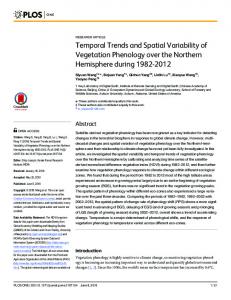
period. By including stations from many different time periods, Legates & Willmott implicitly assumed that resolving more spatial variability was preferable to having a fixed base period (i.e. that spatial interpolation was less reliable than temporal substitution). Since the Legates & Willmott climatology is perhaps the most widely used representation of globalscale air temperature, it is useful to evaluate this assumption. In an analysis of 10-, 20-, and 30-yr averages of annual total precipitation for the USA, Willmott et al. (1996) demonstrated that spatial interpolation introduces much larger errors than does using data from different base periods (i.e. temporal substitution). Hulme & New (1997), however, in comparing precipitation averages from 1931–1960 and Fig. 1. Hypothetical examples of aliasing in spatial cross-sections in both (a) a 1961–1990, found large relative differtraditional regular sampling context and (b) an irregular sampling context. ences between these time periods in Aliasing is typically discussed in a temporal framework, but similar transfer of tropical North Africa (where precipismall-scale information (dashed line) to larger-scale ‘information’ (solid line) tation is inherently low and varies occurs when analyzing spatial data. Sparse climatological networks are particularly susceptible to problems associated with aliasing considerably on decadal scales) but not in Europe. Since air temperature typically is less spatially variable than Hansen & Lebedeff 1987) to reduce spatial variability precipitation, it might be assumed that increased spaof air temperature. As a result, air temperature anomtial resolution of air temperature would not be preferalies have much lower spatial variability than actual air able to maintaining a standard base period. Legates & temperatures and, therefore, are easier to analyze spaWillmott, however, assumed the opposite and included tially. For applications such as comparisons with global many stations with air temperature averages derived climate model output and environmental modeling, from different base periods. As a result, this research however, the spatial variability of actual air temperaseeks to compare spatial and temporal variability of ture is of fundamental interest and must be estimated. multiyear averages of monthly and annual average air Another reason for comparing spatial and temporal temperature to assess these assumptions. Both tradivariability is more practical and is related to the compitional spatial interpolation and a method that utilizes lation of climatological means or ‘normals’ of air temelevation data and standard atmospheric lapse rates perature. Within such climatologies, station data usuare used to evaluate unresolved spatial variability. ally are analyzed only within a standard base period (e.g. 1961 to 1990) and station records that do not contain sufficient data during the base period are removed 2. MONTHLY AIR TEMPERATURE IN THE (e.g. Hulme et al. 1995). If between-station variability is CONTIGUOUS UNITED STATES of interest (e.g. a map or gridded field of climatological mean air temperature is needed), then removing such 2.1. Data: preprocessing and resulting network stations assumes that spatial interpolation between stations is more reliable than using a temporal mean from To properly compare spatial and temporal varia shorter or different averaging period. Using a temability, a surface station network that is both spatially poral mean from a different base period (e.g. using the dense and temporally extensive is needed. A high1941–1970 average as an estimate of the 1961–1990 quality data set that fulfills these requirements is the average) is a process that we call ‘temporal substitution’. United States Historical Climatology Network (HCN; In developing a global climatology of air temperaEasterling et al. 1996). The HCN contains 1221 stations ture, Legates & Willmott (1990) included all stations with at least 80 yr of monthly mean surface air temthat had monthly averages available for at least a 10-yr perature records (Fig. 2a). The resolution of the HCN is
Robeson & Janis: Time-averaged air temperature
17
tween 1921 and 1994 were available. The 80% dataavailable criterion was chosen as a tradeoff between temporal fidelity and spatial resolution. Using only those stations with no missing values would limit spatial resolution to less than 100 stations. Using a 90% data-available criterion would result in approximately 400 stations while going to an 80% criterion resulted in a network that contains 720 stations with an average distance to nearest neighbor of 59 km and a network density of 91 stations per 106 km2. Further examination of missing values shows that on any given month from 1921 to 1994, the 80% criterion produces a network that rarely has 10 stations missing and never more than 27, indicating that the issue of estimating a 10-yr average from 8 or 9 yr of data is not a widespread problem. The resulting 720-station network (Fig. 2b) is fairly well-distributed throughout much of the eastern and midwestern USA, but is more sparse and uneven in the west, particularly in the southwest. The lower station density in the southwest does not hinder our analyses in general, yet may make conclusions drawn about this region less definitive.
Fig. 2. Spatial distribution of air temperature stations in (a) the Historical Climate Network (1221 stations) and in (b) a subnetwork of 720 HCN stations that have at least 80% data available in all 10-yr periods from 1921 to 1994
relatively high throughout much of the contiguous USA except for parts of the west. The HCN data package contains, in addition to original monthly averages, adjustments for time-of-observation bias, station moves, instrument changes and various other inhomogeneities (e.g. Karl et al. 1986, Karl & Williams 1987). Many of these adjustments, with the exception of time-ofobservation bias, may contain interstation dependencies (i.e. corrections based on spatial relationships between stations) that may not allow for a fair comparison of spatial and temporal variability; therefore, data with only time-of-observation bias adjustments will be used. While data-quality issues are critical and relevant to this research (since they influence both spatial and temporal variability), our focus on multiyear air temperature averages helps to reduce the impacts of data problems [in addition, many of the differences that we show (Section 4) are sufficiently large that data-quality issues would not alter them]. The length of the study was constrained to the period 1921 to 1994 such that the network was spatially dense while minimizing the potential for missing values. No station was included in our study unless, for all months, at least 80% of the data from every 10-yr period be-
2.2. Spatial variability of annual, January, and July air temperature Since the results of our analyses will primarily be represented by error maps and spatially averaged statistics, it is necessary to briefly discuss the inherent spatial variability of mean air temperature fields at their highest spatial resolution. From the 1221 station HCN (Fig. 2a), 1961–1990 average annual, January, and July air temperature were interpolated to the nodes of a 0.25° × 0.25° latitude-longitude grid using the spherical spatial interpolation method of Willmott et al. (1985). Across the contiguous USA, maps of mean air temperature are dominated by well-known relationships with latitude, elevation, and proximity to coasts (Fig. 3). Spatial gradients of air temperature are generally more coherent (and larger) for annual and January averages than for July averages, but mountainous areas have relatively high spatial variability regardless of season. July average air temperature varies spatially by less than 10°C throughout much of the east while values in the west vary by over 25°C (although the network density certainly causes underestimation of spatial variability in the west). Greater spatial variability in the west is due mostly to variations in elevation, which force temperature both directly (via lapse rates) and indirectly (via cloud cover, humidity, etc.). Since variations in both elevation and network density have important implications for estimating the spatial variability of air temperature, both will be addressed explicitly in our analyses.
18
Clim Res 10: 15–26, 1998
3. METHODS FOR ESTIMATING SPATIAL AND TEMPORAL VARIABILITY
(a) To compare the relative magnitudes of spatial and temporal variability, 2 distinct approaches are used: spatial interpolation and temporal substitution (Fig. 4). Below, the 2 approaches are outlined and contrasted.
3.1. Spatial interpolation
(b)
Since one of the goals of this research is to evaluate whether it is necessary to remove stations that do not have complete records during a specific base period (e.g. 1961 to 1990), the spatial interpolation approach used here emulates the process of removing stations from a climatology. To generate errors that result from spatially interpolating to unsampled locations (i.e. culled stations), a station is removed and surrounding stations are used to estimate the station’s annual and monthly mean air temperature (Fig. 4a). This ‘crossvalidation’ process (Efron & Gong 1983) is repeated for each station in the network, producing a set of errors
(c)
Fig. 3. (a) Annual, (b) January, and (c) July air temperature (°C) for the period 1961 to 1990. Note that different color scales are used on each map
Fig. 4. Schematic depiction of the research methods used to estimate unresolved spatial and temporal variability. For unresolved spatial variability, spatial interpolation and cross validation, depicted in (a), are used such that a station is removed (e.g. the central station with the open circle, in this case) and its air temperature is estimated via spatial interpolation from data at surrounding locations. This interpolation/cross-validation process is repeated for all averaging periods from 1920 to 1994, allowing error statistics to be calculated at each station. To estimate temporal variability, temporal substitution, depicted in (b), uses values from all other averaging periods to estimate the value of a given base period [in this case, the ‘observed’ value is the 1961 to 1970 air temperature average at the same station as in (a)]. Each specific averaging period that is used as an ‘observed’ value has error statistics (such as mean absolute error, MAE) associated with it. The error statistics themselves then can be averaged (over all averaging periods used as ‘estimates’) to produce a single error statistic (at each station) that is directly comparable to that produced by spatial interpolation/cross-validation
Robeson & Janis: Time-averaged air temperature
(derived from all possible m-year time periods from 1921 to 1994) at each station. Cross validation is independent of any particular interpolation method and therefore provides a general technique for evaluating spatial variability and spatial interpolation errors (Isaaks & Srivastava 1989, Robeson 1994), although some care should be taken not to overinterpret crossvalidation errors (Davis 1987). In general, overinterpretation of cross-validation errors occurs when comparing small differences between competing methods. A large number of spatial interpolation methods are available (Lam 1983, Bennett et al. 1984, Thiébaux & Pedder 1987, Robeson 1997), all of which estimate values at unsampled locations using some or all of the data available. For this research, an accurate and computationally efficient method is advantageous. When performing the large number of interpolations that cross validation requires, a local procedure (i.e. one that utilizes a ‘local’ subset of the data to estimate values at unsampled locations) is most efficient. In addition, the procedure should incorporate spherical geometry in order to minimize errors resulting from inaccurate distance calculations (Robeson 1997). One method that has these properties is the spherical version of Shepard’s (1968) algorithm implemented by Willmott et al. (1985). The spherical implementation of Shepard’s method is fundamentally a version of inverse-distance weighting; however, it does incorporate separate weighting functions that account for clustering of data points and allow for extrapolation. The algorithm of Willmott et al. (1985) has been used extensively to interpolate climatological data (e.g. Legates & Willmott 1990, Willmott et al. 1994, Huffman et al. 1995, Robeson 1995). It also has been shown to be fast and accurate (Bussières & Hogg 1989, Robeson 1994), especially for nonsmooth data (Robeson 1997). While univariate spatial interpolation is commonly used to generate gridded fields and to perform cross validation, nearly all methods of spatial interpolation can be improved if the relationships between the variable of interest and other higher-resolution spatial fields are incorporated. For air temperature, the most appropriate higher-resolution field is a digital elevation model or DEM (Willmott & Matsuura 1995, Dodson & Marks 1997). Using atmospheric lapse rates, station air-temperature data from differing elevations can be brought to a common elevation, interpolated to the nodes of a DEM grid, and transformed to actual air temperatures using the gridded digital elevation data. This procedure has been shown to be more accurate than univariate interpolation and has been referred to as ‘DEM-aided interpolation’ (Willmott & Matsuura 1995) and the ‘linear lapse rate adjustment’ (Dodson & Marks 1997). To parallel the term ‘climatologically aided interpolation’ (CAI) introduced by Willmott &
19
Robeson (1995), however, we prefer the term ‘topographically aided interpolation’ (TAI). Cross validation can be easily implemented within the TAI framework by successively removing stations and using station elevations to estimate station air temperatures from the common-elevation interpolation. CAI (Willmott & Robeson 1995), which is a method that uses anomalies to ‘update’ a high-resolution climatology [e.g. Legates & Willmott (1990), or one derived from a specific base period], will not be used here since it is a hybrid approach (incorporating elements of temporal substitution with traditional spatial interpolation) that combines the 2 separate errors that we are trying to estimate. We do know, however, from the work of Willmott & Matsuura (1995) that TAI performs as well as or better than CAI for annual average air temperature in the USA. In implementing CAI, overall error can be thought of as having 3 somewhat distinct components: (1) error from using averages from varying time periods in the high-resolution climatology, (2) errors in interpolating the climatology, and (3) errors in interpolating the anomalies that are used to update the climatology. The research presented here addresses the first 2 errors while Robeson (1994) addressed the third.
3.2. Temporal substitution To estimate temporal variability, 5-, 10-, and 30-yr averages from the same time periods used in the spatial interpolation analysis are compared. If 10-yr base periods are being examined, for example, then the air temperature average over a particular 10-yr period (e.g. 1961 to 1970) is treated as the ‘observed’ value. All other 10-yr periods from 1921 to 1994 are used as estimated values which are compared with the ‘observed’ value to generate an error distribution at each station (Fig. 4b). We refer to this process as ‘temporal substitution’ because it emulates the errors generated in substituting climatic averages from nonstandard base periods for those of standard base periods (as opposed to the more-accepted approach of excluding stations and interpolating to that location).
4. SPATIAL VERSUS TEMPORAL VARIABILITY At each station used in our analysis (Fig. 2b), ‘observed’ and ‘estimated’ values can be generated using the spatial interpolation and temporal substitution procedures outlined above (Section 3). In the case of the spatial interpolation methods, cross validation (Fig. 4a) then is used to generate an estimated value at each station for all possible m-year base periods (where m is
20
Clim Res 10: 15–26, 1998
5, 10, or 30), producing a mean absolute error (s MAEj, where s denotes ‘spatial’) at each station j: s MAE j
=
1 nm
∑k =1 Tj ,k nm
^
− T j ,k
(1)
where nm is the number of different base periods for an m-year average (70 for 5-yr averages, 65 for 10-yr averages, and 45 for 30-yr averages), T^j,k is the crossvalidation estimated air temperature for station j and base period k, and Tj,k is the observed air temperature. In this way, an MAE can be generated for both the traditional interpolation method and TAI. When using temporal substitution, the same Tj,k serves as the observed value, but all other nm – 1 base periods are used as the estimated values. For example, if the 1961 to 1970 period is selected as the ‘observed’ period under the spatial interpolation procedure, then all 64 other 10-yr periods are used as the ‘estimated’ value. As a result, each time period k (at each station j ) has an associated MAE (denoted as MAEj,k in Eq. 2). The MAEj,k are averaged at the station to produce an MAEj for temporal substitution: t MAE j
∑k =1 MAE j ,k
=
1 nm
=
nm nm ^ 1 Tj , l − Tj , k l ≠ k nm (nm − 1) ∑k =1 ∑l =1
nm
(2)
where t MAEj is the temporal substitution MAE for station j. So, although the procedure for producing an MAE at each station j is slightly different for spatial interpolation and temporal substitution, the 2 errors are directly comparable since the ‘observed’ variable is the same in both cases (Tj,k).
4.1. Error maps The mean absolute errors at each station (MAEj ) for traditional spatial interpolation, TAI, and temporal substitution are gridded (on a 0.25° × 0.25° latitudelongitude grid), mapped, and compared for annual and monthly air temperatures. Five-, 10-, and 30-yr base periods are used; however, maps are only shown for annual, January, and July 10-yr periods (see Figs. 5 to 7) since 10-yr periods tend to show more interesting spatial patterns than 30-yr periods (which have substitution errors that are low everywhere) and are more commonly used than 5-yr periods in large-scale climatologies. Overall, MAEs for 10-yr averages of annual air temperature using the substitution method are much lower than for either of the interpolation methods (Fig. 5). No part of the USA has large substitution errors for 10-yr periods, while large areas in the western USA and isolated parts of the east have very large interpolation
errors (over 2°C). The maximum MAE for 10-yr averages of annual air temperature at any grid point for interpolation is 8.44°C, while for substitution, the maximum MAE at any grid point is less than 1°C (see Table 1). TAI reduces interpolation error, but, overall, substitution errors are still lower (compare Fig. 5b and c). Since 10-yr averages of annual mean air temperature have much lower substitution errors than interpolation errors, it is implied that unresolved spatial variability of 10-yr averages of annual mean air temperature across the USA is much larger than temporal variability of 10-yr averages. While much of the unresolved spatial variability is concentrated in the western USA, TAI only resolves part of the spatial variability, indicating that more than the elevation/ lapse-rate relationship is responsible for the unresolved spatial variability of annual mean air temperature (e.g. cloud cover, advection, sparser network). Since further smoothing of the temporal variability, such as going from 10-yr averages to 30-yr averages, will inevitably reduce substitution error, 30-yr averages of annual air temperature also show that temporal substitution generally performs much better than spatial interpolation (Table 1). Maps of 5-yr averages of annual air temperature (not shown) also have substitution errors that are lower than either interpolation method. When monthly data are used to generate error maps for 10-yr averages, substitution performs less impressively, particularly during January (see Fig. 6). Both spatial interpolation methods (Fig. 6a, b) produce January MAE patterns and magnitudes that are similar to those for annual air temperature. The temporal substitution process, however, produces much larger errors for January than for annual data (compare Fig. 5c to Fig. 6c; also, see Table 1). Mean absolute error maps for January using substitution (Fig. 6c) show large errors in the northern Great Plains and throughout much of the eastern portion of the country (excluding northern New England, northern Michigan, and southern Florida). The Great Plains and the eastern USA clearly have larger temporal variability of air temperature than other areas of the country during January (due to intermittent intrusions of both arctic and subtropical air). Temporal substitution, therefore, performs poorly in regions (and at times of year) where there is large interannual variability in synoptic-scale systems (i.e. the forcing mechanism with the largest interannual variability). Areas such as northern New England, northern Michigan, and southern Florida, however, have the moderating influence of water (albeit very different water bodies) to reduce interannual temporal variability. On maps of substitution error for 5-yr averages of January air temperature (not shown), extensive areas of large error in the north-
Robeson & Janis: Time-averaged air temperature
where MAE is the spatially averaged mean absolute error, MAEi is the gridded error at grid point i, φi is the latitude of grid point i, and ng is the number of grid points. Spatially averaged interpolation errors, in general, do not vary greatly 30-yr Mean Max. from month to month, although interpolation errors typically are lowest in spring and fall (Fig. 8). Spatially aver1.00 8.46 aged temporal-substitution errors are 0.67 3.32 0.22 1.01 more closely related to time of year, with winter months producing much 1.10 8.00 larger errors, particularly for 5- and 0.88 4.91 10-yr averages (Fig. 8a, b). For 30-yr 0.60 1.39 averages, temporal substitution pro1.15 9.72 duces lower overall errors than either 0.79 9.81 spatial interpolation method at all 0.28 0.76 times of year (Fig. 8c). For 10-yr averages, TAI reduces interpolation errors to a level where TAI would be preferred (over temporal substitution) during January, February, and March. In addition, TAI of 5-yr averages produces lower spatial interpolation errors than temporal substitution for nearly all months, again with greatest differences occurring in winter. It appears, therefore, that the ‘cutoff’ averaging length, where temporal variability exceeds spatial variability, is somewhere between 5 and 10 yr. Narrowing this cutoff further, however, would overemphasize spatially averaged errors, which we clearly should not do, since the spatial patterns of error for the various methods clearly are different (Figs. 5 to 7). In addition, (1) overemphasizing relatively small cross-validation differences is not recommended and (2) our results are networkdependent (see Section 4.3). To summarize, when developing a climatology that is used to depict the spatial variability of monthly air temperature in the USA, including a climatological mean from all stations with 10 or more years of data appears to be preferable to removing stations that do not have sufficient data during a specific base period, except during winter months. If high-quality climate stations have 30 or more years of data, their data should nearly always be included in the climatology. If only a short record (1°C) over extensive sections of the northcentral and eastern USA. During most months, temporal substitution errors are low throughout the contiguous USA, while spatial interpolation errors are largest in areas with large elevation differences, despite using an interpolation procedure that incorporates standard lapse rates and elevation data (TAI). TAI of 5-yr averages of monthly air temperature produces lower errors than temporal substitution for nearly all months (but not for annual averages), suggesting that, in general, multiyear monthly air temperature averages shorter than 10 yr in length should not be ‘substituted’ into a long-term climatology. It is important to emphasize, however, that these results (1) apply only to the contiguous USA and (2) only refer to spatially averaged errors (i.e. not errors at any given location). Further implications of this research include: (1) areas of high relief need to have extensive station networks even when using interpolation methods that include elevation data and (2) methods that better resolve the spatial variability of air temperature are needed. While ‘smart’ interpolation methods (e.g. Hutchinson 1995, Willmott & Matsuura 1995, Dodson & Marks 1997) such as TAI are being used increasingly, there still is a need for improved spatial interpolation methods. One possibility is to make better use of satellite-observed data, in order to derive high-resolution fields that are closely
25
related to surface fields. In addition to signaling the need for better spatial representations of air temperature, this research (and the work of Hulme & New 1997) suggests that comparisons of temporal and unresolved variability are needed in many different climatic regimes. Regions of the world with large (or small) interannual variability or low (or high) relief will have fundamentally different relationships between spatial and temporal variability. Comparisons of spatial interpolation and temporal substitution in high- and low-latitude areas should provide additional insight into the fundamental variability of air temperature.
LITERATURE CITED Bennett RJ, Haining RP, Griffith DA (1984) The problem of missing data on spatial surfaces. Ann Assoc Am Geogr 74:138–156 Brinkmann WAR (1983) Variability of temperature in Wisconsin. Mon Weath Rev 111:172–179 Bussières N, Hogg W (1989) The objective analysis of daily rainfall by distance weighting schemes on a mesoscale grid. Atmos Ocean 27:521–541 Davis BM (1987) Uses and abuses of cross-validation in geostatistics. Math Geol 19:241–248 Diaz HF, Quayle RG (1980) The climate of the United States since 1895: spatial and temporal changes. Mon Weath Rev 108:249–266 Dodson R, Marks D (1997) Daily air temperature interpolated at high spatial resolution over a large mountainous region. Clim Res 8:1–20 Easterling DR, Karl TR, Manson EH, Hughes PY, Bowman DP (1996) United States Historical Climatology Network (U.S. HCN) Monthly Temperature and Precipitation Data. NDP019/R3, ORNL/CDIAC-87. Carbon Dioxide Information and Analysis Center, Oak Ridge National Laboratory, Oak Ridge, TN Efron B, Gong G (1983) A leisurely look at the bootstrap, the jackknife, and cross-validation. Am Statistician 37:36–48 Hansen J, Lebedeff S (1987) Global trends of measured surface air temperature. J Geophys Res 92(D11):13345–13372 Huffman GJ, Adler RF, Rudolf B, Schneider U, Keehn PR (1995) Global precipitation estimates based on a technique for combining satellite-based estimates, rain gauge analysis, and NWP model precipitation information. J Clim 8:1284–1295 Hulme M, Conway D, Jones PD, Jiang T, Barrow EM, Turney C (1995) Construction of a 1961–1990 European climatology for climate change modelling and impact applications. Int J Climatol 15:1333–1363 Hulme M, New M (1997) Dependence of large-scale precipitation climatologies on temporal and spatial sampling. J Clim 10:1099–1113 Hutchinson MF (1995) Interpolating mean rainfall using thin plate smoothing splines. Int J Geogr Inf Sys 9:385–403 Isaaks EH, Srivastava RM (1989) Applied geostatistics. Oxford University Press, New York Jones PD, Raper SCB, Bradley RS, Diaz HF, Kelly PM, Wigley TML (1986) Northern Hemisphere surface air temperature variations: 1851–1984. J Clim Appl Meteorol 25:161–179 Karl TR, Williams CN Jr (1987) An approach to adjusting climatological time series for discontinuous inhomogeneities. J Clim Appl Meteorol 26:1744–1763
≤ 26
Clim Res 10: 15–26, 1998
Karl TR, Williams CN Jr, Young PJ, Wendland WM (1986) A model to estimate the time of observation bias associated with monthly mean maximum, minimum, and mean temperatures for the United States. J Clim Appl Meteorol 25: 145–160 Lam NSN (1983) Spatial interpolation methods: a review. Am Cartographer 10:129–149 Legates DR, Willmott CJ (1990) Mean seasonal and spatial variability in global surface air temperature. Theor Appl Climatol 41:11–21 Madden RA, Shea DJ (1978) Estimates of the natural variability of time-averaged temperatures over the United States. Mon Weath Rev 106:1695–1703 Robeson SM (1994) Influence of spatial sampling and interpolation on estimates of terrestrial air temperature change. Clim Res 4:119–126 Robeson SM (1995) Resampling of network-induced variability in estimates of terrestrial air temperature change. Clim Change 29:213–229 Robeson SM (1997) Spherical methods for spatial interpolation: review and evaluation. Cartogr Geogr Inf Sys 24:3–20 Shepard D (1968) A two-dimensional interpolation function for irregularly spaced data. Proc 23rd Natl Conf ACM,
Association for Computing Machinery, New York, p 517–523 Thiébaux HJ, Pedder MA (1987) Spatial objective analysis. Academic Press, New York Vining KC, Griffiths JF (1985) Climatic variability at ten stations across the United States. J Clim Appl Meteorol 24:363–370 Willmott CJ, Matsuura K (1995) Smart interpolation of annually averaged air temperature in the United States. J Appl Meteorol 34:2577–2586 Willmott CJ, Robeson SM (1995) Climatologically aided interpolation (CAI) of terrestrial air temperature. Int J Climatol 15:221–229 Willmott CJ, Robeson SM, Feddema JJ (1994) Estimating continental and terrestrial precipitation averages from raingauge networks. Int J Climatol 14:403–414 Willmott CJ, Robeson SM, Janis MJ (1996) Comparison of approaches for estimating time-averaged precipitation using data from the USA. Int J Climatol 16:1103–1115 Willmott CJ, Rowe CM, Philpot WD (1985) Small-scale climate maps: a sensitivity analysis of some common assumptions associated with grid-point interpolation and contouring. Am Cartographer 12:5–16
Editorial responsibility: Laurence Kalkstein, Newark, Delaware, USA
Submitted: June 2, 1997; Accepted: January 7, 1998 Proofs received from author(s): March 17, 1998