competition and cooperation in supply chains: game ...

COMPETITION AND COOPERATION IN SUPPLY CHAINS: GAME-THEORETIC MODELS

COMPETITION AND COOPERATION IN SUPPLY CHAINS: GAME-THEORETIC MODELS

By MINGMING LENG, M.Sc.

A Thesis Submitted to the School of Graduate Studies in Partial Fulfillment of the Requirement for the Degree Doctor of Philosophy

McMaster University © Copyright by Mingming Leng, April 2005

Mingming Leng

DeGroote School of Business

DOCTOR OF PHILOSOPHY (2005)

McMaster University Hamilton, Ontario

MASTER OF SCIENCE (1996)

Wuhan University of Technology Wuhan, P. R. China

BACHELOR OF SCIENCE (1993)

Shenyang Institute of Technology Shenyang, P. R. China

TITLE:

Competition and Cooperation in Supply Chains: Game-Theoretic Models

AUTHOR:

Mingming Leng

SUPERVISOR:

Professor Mahmut Parlar

SUPERVISORY COMMITTEE:

Professor Mahmut Parlar (Chairman) Assistant Professor Elkafi Hassini Assistant Professor Peter McCabe

NUMBER OF PAGES:

x, 133

ii

Mingming Leng


Abstract In this thesis we focus on applications of game theory in supply chain management (SCM). Most significant–and interesting–topics arising in SCM are concerned with the coordination/cooperation and competition among supply chain members. Since the theory of non-cooperative and cooperative games is used for the analysis of situations involving conflict and cooperation, it has become a commonly-used methodological tool in investigating supply chain-related problems. We start with an introduction in Chapter 1. In this chapter, we briefly describe game theory and SCM, and the organizational structure of this thesis. Next, we present a literature review for game theoretical applications in SCM in Chapter 2. This chapter reviews more than 130 papers concerned with supply chain-related game models, which are categorized based on a topical classification scheme. In Chapter 3, we consider a free shipping problem in a B2B setting. We model the problem as a leader-follower game under complete information with a seller as the leader and a buyer as the follower, and compute the Stackelberg solution for this game. In Chapter 4, we analyze the problem of allocating cost savings in a three-level supply chain involving a supplier, a manufacturer and a retailer. We use concepts from the theory of cooperative games to find allocation schemes for dividing the total cost savings among the three members. Chapter 5 considers game-theoretic models of lead-time reduction in a two-level supply chain involving a manufacturer and a retailer. In this chapter, we first develop a leader-follower game where the manufacturer determines the components of his lead-time and the retailer decides on her order quantity. This game is solved to find the Stackelberg equilibrium. We also investigate the cooperation between the two members and design a linear side-payment contract for this supply chain. Our thesis ends with a conclusion in Chapter 6.

iii

Mingming Leng


Acknowledgements I am particularly grateful to my supervisor, Professor Mahmut Parlar, who contributed tremendously to my knowledge in management science area, provided considerable insightful comments for improving my thesis, and generously spent his time with me. I will like to thank Drs. Elkafi Hassini and Peter McCabe for their careful review of the manuscript and many helpful comments. I am also indebted to Ontario Student Assistance Program and McMaster University for providing financial assistance during my Ph.D. study. This thesis is dedicated to my family for their encouragement and support throughout the four years.

iv

Mingming Leng


Contents 1 Introduction . . . . . . . . . . . . . . . . . . . . . . . . . . . . . . . . . . . . . . . . . . . . . . . . . . . . . . . . . . . . . . . . . . . 1 1.1 Game Theory and Supply Chain Management. . . . . . . . . . . . . . . . . . . . . . . . . . . . . . 1 1.2 Organization and Overview . . . . . . . . . . . . . . . . . . . . . . . . . . . . . . . . . . . . . . . . . . . . . . . . . 3 2 Game Theoretic Applications in SCM1 . . . . . . . . . . . . . . . . . . . . . . . . . . . . . . . . . . . . 5 2.1 Concepts in Game Theory and Topical Classification of Supply Chain-Related Problems . . . . . . . . . . . . . . . . . . . . . . . . . . . . . . . . . . . . . . . . . . . . . . . . . . . . 5 2.1.1 Brief Review of Some Solution Concepts in Game Theory . . . . . . . . . . . 6 2.1.2 Topical Classification of SCM-related Problems. . . . . . . . . . . . . . . . . . . . . 15 2.2 Inventory Games with Fixed Unit Purchase Cost . . . . . . . . . . . . . . . . . . . . . . . . . . 15 2.3 Inventory Games with Quantity Discounts . . . . . . . . . . . . . . . . . . . . . . . . . . . . . . . . 19 2.4 Production and Pricing Competition . . . . . . . . . . . . . . . . . . . . . . . . . . . . . . . . . . . . . . 22 2.5 Games with Other Attributes . . . . . . . . . . . . . . . . . . . . . . . . . . . . . . . . . . . . . . . . . . . . . . 26 2.5.1 Capacity Decisions . . . . . . . . . . . . . . . . . . . . . . . . . . . . . . . . . . . . . . . . . . . . . . . . . . 26 2.5.2 Service Quality. . . . . . . . . . . . . . . . . . . . . . . . . . . . . . . . . . . . . . . . . . . . . . . . . . . . . . 27 2.5.3 Product Quality . . . . . . . . . . . . . . . . . . . . . . . . . . . . . . . . . . . . . . . . . . . . . . . . . . . . 28 2.5.4 Advertising and New Product Introduction . . . . . . . . . . . . . . . . . . . . . . . . . 29 2.6 Games with Joint Decisions on Inventory, Production/Pricing and Other Attributes . . . . . . . . . . . . . . . . . . . . . . . . . . . . . . . . . . . . . . . . . . . . . . . . . . . . . . . . . . . 30 2.6.1 Joint Inventory and Production/Pricing Decisions . . . . . . . . . . . . . . . . . . 31 2.6.2 Joint Inventory and Capacity Decisions . . . . . . . . . . . . . . . . . . . . . . . . . . . . . 32 2.6.3 Joint Production/Pricing and Capacity Decisions. . . . . . . . . . . . . . . . . . . 33 2.6.4 Joint Production/Pricing and Service/Product Quality Decisions . . 34 2.6.5 Joint Production/Pricing and Advertising/New Product Introduction Decisions . . . . . . . . . . . . . . . . . . . . . . . . . . . . . . . . . . . . . . . . . . . . . . 35 2.7 Conclusion and Further Discussion . . . . . . . . . . . . . . . . . . . . . . . . . . . . . . . . . . . . . . . . 36 3 Free Shipping and Purchasing Decisions in B2B Transactions: A 1

This chapter has been accepted by INFOR for publication.

v

Mingming Leng


Game-Theoretical Analysis2 . . . . . . . . . . . . . . . . . . . . . . . . . . . . . . . . . . . . . . . . . . . . . . . .38 3.1 Introduction . . . . . . . . . . . . . . . . . . . . . . . . . . . . . . . . . . . . . . . . . . . . . . . . . . . . . . . . . . . . . . . 38 3.2 Objective Functions of the Players. . . . . . . . . . . . . . . . . . . . . . . . . . . . . . . . . . . . . . . . . 41 3.3 Buyer’s Best Response Function . . . . . . . . . . . . . . . . . . . . . . . . . . . . . . . . . . . . . . . . . . . 44 3.4 Stackelberg Solution . . . . . . . . . . . . . . . . . . . . . . . . . . . . . . . . . . . . . . . . . . . . . . . . . . . . . . . 50 3.4.1 Stackelberg Solution When C(y) and V (y) Intersect Once . . . . . . . . . . 51 3.4.2 Stackelberg Solution When C(y) and V (y) Intersect More Than Once . . . . . . . . . . . . . . . . . . . . . . . . . . . . . . . . . . . . . . . . . . . . . . . . . . . . . . . . . . 52 3.5 Sensitivity Analysis . . . . . . . . . . . . . . . . . . . . . . . . . . . . . . . . . . . . . . . . . . . . . . . . . . . . . . . . 55 3.6 Summary and Concluding Remarks. . . . . . . . . . . . . . . . . . . . . . . . . . . . . . . . . . . . . . . . 57 4 Allocation of Cost Savings in a Three-Level Supply Chain with Demand Information Sharing: A Cooperative-Game Approach . . . . . . .59 4.1 Introduction . . . . . . . . . . . . . . . . . . . . . . . . . . . . . . . . . . . . . . . . . . . . . . . . . . . . . . . . . . . . . . . 59 4.2 Literature Review. . . . . . . . . . . . . . . . . . . . . . . . . . . . . . . . . . . . . . . . . . . . . . . . . . . . . . . . . . 63 4.3 Information Sharing and Expected Costs for Different Coalitional Structures. . . . . . . . . . . . . . . . . . . . . . . . . . . . . . . . . . . . . . . . . . . . . . . . . . . . . . . . . . . . . . . . . . 65 4.3.1 Retailer’s Expected Cost π R . . . . . . . . . . . . . . . . . . . . . . . . . . . . . . . . . . . . . . . . 69 4.3.2 Manufacturer’s Expected Cost . . . . . . . . . . . . . . . . . . . . . . . . . . . . . . . . . . . . . . 71 4.3.3 Supplier’s Expected Cost . . . . . . . . . . . . . . . . . . . . . . . . . . . . . . . . . . . . . . . . . . . 74 4.4 Modeling and Analysis of the Cooperative-Game . . . . . . . . . . . . . . . . . . . . . . . . . . 81 4.4.1 An Information Sharing Cooperative Game in CharacteristicFunction Form . . . . . . . . . . . . . . . . . . . . . . . . . . . . . . . . . . . . . . . . . . . . . . . . . . . . . . 81 4.4.2 Solution of the Cooperative Game . . . . . . . . . . . . . . . . . . . . . . . . . . . . . . . . . . 83 4.5 Numerical Study and Sensitivity Analysis . . . . . . . . . . . . . . . . . . . . . . . . . . . . . . . . . 85 4.6 Conclusion . . . . . . . . . . . . . . . . . . . . . . . . . . . . . . . . . . . . . . . . . . . . . . . . . . . . . . . . . . . . . . . . . 89 5 Lead-Time Reduction in a Two-Level Supply Chain: Stackelberg vs. Cooperative Solution with a Side-Payment Contract . . . . . . . . . . . . . .91 5.1 Introduction . . . . . . . . . . . . . . . . . . . . . . . . . . . . . . . . . . . . . . . . . . . . . . . . . . . . . . . . . . . . . . . 91 5.2 Stackelberg Game. . . . . . . . . . . . . . . . . . . . . . . . . . . . . . . . . . . . . . . . . . . . . . . . . . . . . . . . . . 94 2

This chapter has been accepted by IIE Transactions for publication.

vi

Mingming Leng


5.2.1 The Retailer’s Order Decision. . . . . . . . . . . . . . . . . . . . . . . . . . . . . . . . . . . . . . . 95 5.2.2 The Manufacturer’s Lead-Time Decision . . . . . . . . . . . . . . . . . . . . . . . . . . . . 97 5.2.3 Numerical Example . . . . . . . . . . . . . . . . . . . . . . . . . . . . . . . . . . . . . . . . . . . . . . . . 102 5.3 Cooperation with Side-Payments . . . . . . . . . . . . . . . . . . . . . . . . . . . . . . . . . . . . . . . . . 103 5.3.1 Minimization of the System-Wide Cost . . . . . . . . . . . . . . . . . . . . . . . . . . . . 107 5.3.2 Nash equilibrium . . . . . . . . . . . . . . . . . . . . . . . . . . . . . . . . . . . . . . . . . . . . . . . . . . . 108 5.3.3 Design of the Linear Side-Payment Contract. . . . . . . . . . . . . . . . . . . . . . . 109 5.3.4 Numerical Example . . . . . . . . . . . . . . . . . . . . . . . . . . . . . . . . . . . . . . . . . . . . . . . . 110 5.4 Summary . . . . . . . . . . . . . . . . . . . . . . . . . . . . . . . . . . . . . . . . . . . . . . . . . . . . . . . . . . . . . . . . . 112 6 Summary of Thesis and Concluding Remarks . . . . . . . . . . . . . . . . . . . . . . . . . 113 A Alternative classification . . . . . . . . . . . . . . . . . . . . . . . . . . . . . . . . . . . . . . . . . . . . . . . . . . . . . . 115 A.1 Non-cooperative Game Models . . . . . . . . . . . . . . . . . . . . . . . . . . . . . . . . . . . . . . . . . . . 115 A.2 Cooperative Game Models . . . . . . . . . . . . . . . . . . . . . . . . . . . . . . . . . . . . . . . . . . . . . . . . 116 B Distribution of the Reviewed Papers . . . . . . . . . . . . . . . . . . . . . . . . . . . . . . . . . . . . . . . . . . 117 References . . . . . . . . . . . . . . . . . . . . . . . . . . . . . . . . . . . . . . . . . . . . . . . . . . . . . . . . . . . . . . . . . . . . . 119

vii

Mingming Leng


List of Figures 1

2

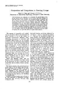
These graphs display the contour curves for each player’s objective function J1 (x1 , x2 ) and J2 (x1 , x2 ). Graphically, the Nash equilibrium is found by superimposing the two figures and finding the intersection of the two lines (which is denoted by a circle •). . . . . . . . . . . . . . . . . . . . . . . . . . . . . . . . . 8

The Pareto optimal solutions P are the collection of points on the thick curve. The Nash arbitrated solution is (f1A , f2A ) ∈ P denoted by the circle • on the curve. . . . . . . . . . . . . . . . . . . . . . . . . . . . . . . . . . . . . . . . . . . . . . . . . . . . . . . . . . . . . . . 11

3

The core of the 3-person game with v(∅) = v(A) = v(B) = v(C) = 0, v(AB) = 2, v(AC) = 4, v(BC) = 6 and v(ABC) = 7 is the area indicated by thick lines. The Shapley value ϕ is outside the core, but the nucleolus ν is inside it. . . . . . . . . . . . . . . . . . . . . . . . . . . . . . . . . . . . . . . . . . . . . . . . . . . . . . . 13

4

When xˆ ≤ v [as in (a)], the buyer’s net revenue function V (y) is maximized at y # = v. But when xˆ ≥ v [as in (b)], the V (y) function is maximized at y # = xˆ. . . . . . . . . . . . . . . . . . . . . . . . . . . . . . . . . . . . . . . . . . . . . . . . . . . . . . . . 45

5

The C(y) + V (ˆ x) curve does not intersect V (y).. . . . . . . . . . . . . . . . . . . . . . . . . . . . . 47

6

The C(y) + V (ˆ x) curve intersects V (y) at two points y1 and y2 . . . . . . . . . . . . . 48

7

Buyer’s best response yR (in $ ) following the seller’s free shipping cutoff level announcement of xˆ. . . . . . . . . . . . . . . . . . . . . . . . . . . . . . . . . . . . . . . . . . . . . . . . . . . . . 49

8

The C(y) + V (τ ) and V (y) curves are tangent for some τ in the interval [v, y¯]. . . . . . . . . . . . . . . . . . . . . . . . . . . . . . . . . . . . . . . . . . . . . . . . . . . . . . . . . . . . . . . . . . . . . . . . . 53

9

Stackelberg strategies xS and yS when c is varied over (0, 0.6). Regions 1 and 2 are defined, respectively, as the intervals (0, c1 ) and (c1 , 0.6) where c1 = 0.49106. . . . . . . . . . . . . . . . . . . . . . . . . . . . . . . . . . . . . . . . . . . . . . . . . . . . . . . . . . . . . . . . . 55

10

Objective functions of the two players for different values of the unit shipping cost c. Regions 1 and 2 are defined, respectively, as the intervals (0, c1 ) and (c1 , 0.6) where c1 = 0.49106.. . . . . . . . . . . . . . . . . . . . . . . . . . . . . . . . . . . . . . 56

11

Order, product and information flows in the three-level supply chain. . . . . . . . 62

12

The transportation and production/processing lead-times. . . . . . . . . . . . . . . . . . . 67

13

Information sharing possibilities for retailer R (Case a) and manufacturer M (Cases b and c) under different coalitional structures. (See text for detailed descriptions of each case.) . . . . . . . . . . . . . . . . . . . . . . . . . . . . . . . . . . . . . . . . . . 68

viii

Mingming Leng


14

Information sharing possibilities for supplier S under different coalitional structures. (See text for detailed descriptions of each case.) . . . . . . . . . . . . . . . . . 69

15

Core, the unstable Shapley value (ϕS , ϕM , ϕR ) = (25.84, 14.63, 18.51) and the constrained nucleolus solution (ν S , ν M , ν R ) = (42.27, 8.355, 8.355) of the game in Example 8. The core is indicated by the thick dotted line and the sides of the triangle. The unstable Shapley value is the empty square (¤) which is outside of the reduced core and the constrained nucleolus is the empty circle (°). . . . . . . . . . . . . . . . . . . . . . . . . . . . . . . . . . . . . . . . . . . . 87

16

The impact of ρ on the constrained nucleolus solution. . . . . . . . . . . . . . . . . . . . . . . 88

17

The impact of ρ on percentage of allocated cost savings at each level. . . . . . . 89

18

The manufacturer’s production process and the retailer’s ordering process. . 94

19

Percentages of the reviewed papers published during the six five-year periods. . . . . . . . . . . . . . . . . . . . . . . . . . . . . . . . . . . . . . . . . . . . . . . . . . . . . . . . . . . . . . . . . . . . . . 118

20

Distribution of the reviewed papers in the five classes. The five classes are: (i) Inventory games with fixed unit purchase cost, (ii) Inventory games with quantity discounts, (iii) Production and pricing competition, (iv) Games with other attributes and (v) Games with joint decisions on inventory, production/pricing and other attributes. . . . . . . . . . . . . . . . . . . . . . . . . 118

ix

Mingming Leng


List of Tables 1

Summary of some papers related to production/pricing with constraints. . . . 24

2

Summary of some papers related to advertising decisions. . . . . . . . . . . . . . . . . . . . 30

3

Distribution of the papers reviewed in the survey. Here, the five classes are defined as follows: (i) Inventory games with fixed unit purchase cost, (ii) Inventory games with quantity discounts, (iii) Production and pricing competition, (iv) Games with other attributes and (v) Games with joint decisions on inventory, production/pricing and other attributes. . . . . . . . . . . . 117

x

Mingming Leng


Chapter 1 Introduction This chapter describes game theory and supply chain management (SCM), and also indicates the organizational structure of this thesis. We show in this chapter that the theory of games has broad applications in diverse fields, and particularly plays an increasingly important role in analyzing various competitive and cooperative issues in supply chains. Motived by the description, we focus our attention on supply chainrelated games.

1.1

Game Theory and Supply Chain Management

Game theory is concerned with the analysis of situations involving conflict and cooperation. Since its development in the early 1940s game theory has found applications in diverse areas such as anthropology, auctions, biology, business, economics, management-labour arbitration, philosophy, politics, sports and warfare. After the initial excitement generated by its potential applications, interest in game theory by operations research/management science specialists seemed to have waned during the 1960s and the 1970s. However, the last two decades have witnessed a renewed interest by academics and practitioners in the management of supply chains and a new emphasis on the interactions among the decision makers (“players”) constituting a supply chain. This has resulted in the proliferation of publications in scattered journals dealing with the use of game theory in the analysis of supply chain-related problems. The purpose of this chapter is to provide a wide-ranging survey (of more than 130 papers) focusing on game theoretic applications in different areas of supply chain management (SCM). A supply chain can be defined as “a system of suppliers, manufacturers, distributors, retailers, and customers where materials flow downstream from suppliers to customers and information flows in both directions” (Ganeshan et al. [69] ). Supply chain management, on the other hand, is defined by some researchers as a set of management processes. For example, LaLonde [120] defines SCM as “the process of managing relationships, information, and materials flow across enterprise borders to deliver enhanced customer service and economic value through synchronized management of the flow of physical goods and associated information from sourcing to consumption.” (See Mentzer et al. [151] for a collection of competing definitions.) Adopting LaLonde’s definition, one observes that most SCM-related research has features that are common to operations management and marketing problems, e.g., 1

Mingming Leng


inventory control, production and pricing competition, capacity investments, service and product quality competition, advertising and new product introduction. Several survey papers related to SCM have appeared in the literature. For example, Tayur et al. [201] have edited a book emphasizing quantitative models for SCM. Ganeshan et al. [69] proposed a taxonomic review and framework that help both practitioners and academic researchers better understand the up-to-date state of SCM research. Wilcox et al. [220] presented a brief survey of the papers on the price-quantity discount. McAlister [146] reviewed a model of distribution channels incorporating behavior dimensions. Goyal and Gupta [80] provided a survey of literature that treated buyer-vendor coordination with integrated inventory models. In addition to the above, some reviews focussing on the application of game theory in economics or management science have appeared in the last five decades. An early survey of game theoretic applications in management science was given by Shubik [192]. Feichtinger and Jørgensen [65] published a review that was restricted to differential game applications in management science and operations research. More recently, Wang and Parlar [215] presented a survey of the static game theory applications in management science problems. A review of applications of differential games in advertising was given by Jørgensen [101]. Li and Whang [135] provided a survey of game theoretic models applied in operations management and information systems where the SCM-related literature focusing on information sharing and manufacturing/marketing incentives was also discussed. In addition, several books (e.g., Chatterjee and Samuelson [39], Gautschi [71], Kuhn and Szego [115] and Sheth et al. [191]) partially reviewed some specific game-related topics in SCM. In the last few years two important reviews focussing on game theoretical applications in supply chain management were published. In [33] Cachon and Netessine outlined game-theoretic concepts and surveyed applications of game theory in supply chain management. Cachon and Netessine classified games that were developed for SCM into four categories based on game-theoretical techniques: (i) Non-cooperative static games, (ii) dynamic games, (iii) cooperative games, and (iv) signaling, screening and Bayesian games. In each category, the authors presented the major techniques that are commonly used in the existing papers and those that could be applied in future research. Our review in Chapter 2 differs from Cachon and Netessine [33] because we review about 130 papers based on a classification of SCM topics (rather than game-theoretical techniques). In [25] Cachon reviewed the literature on supply chain collaboration with contracts. Our review in Chapter 2 differs from [25] as we review game models concerned with coordination and competition in supply chains. Moreover, Chapter 2 reviews several very recent papers which were not mentioned in [25] or [33]. Most significant–and interesting–topics arising in SCM emphasize the coor2

Mingming Leng


dination/cooperation and competition among supply chain’s channel members. In a centralized supply chain the “central” decision maker may coordinate the members’ activities to increase the competitive capability of the supply chain. In other words, the single decision maker determines the optimal solution that globally improves the supply chain performance; thus, in these type of centralized problems game theory is not used. However, for a decentralized supply chain where each supply chain member is an independent decision maker, there arise two issues: (i) Supply chain members compete to improve their individual performance. For example, several agents at the same echelon of a supply chain may compete for limited resources or compete for demand from the same group of customers. As a result, various competitive gamerelated issues arise in the analysis of the decentralized supply chains with competition, (ii) Supply chain members may agree to have a contract to coordinate their strategies in order to improve the global performance of the system as well as their individual profits. For this type of decentralized supply chains with cooperation/coordination, channel members may not only achieve supply chain-wide optimization but also they would have no incentives to deviate from the global optimal solution. Naturally, a prime methodological tool for dealing with these problems is non-cooperative and cooperative game theory that focuses on the simultaneous or sequential decision-making of multiple-players under complete or incomplete information.

1.2

Organization and Overview

This thesis is organized as follows. Chapter 2 briefly describes major solution concepts commonly used in the analysis of the non-cooperative and cooperative games, and reviews over 130 papers concerned with applications of game theory in SCM. The concepts which we discuss include: (i) Nash equilibrium and Stackelberg solution in the non-cooperative game theory; and (ii) the core, the Shapley value, the nucleolus, the Nash arbitration scheme and cooperation with side-payments in the theory of cooperative games. Chapter 2 also provides a review of the existing supply chain game models, under a topical classification of five areas where supply chain-related game theoretical applications are found: (i) Inventory control, (ii) production and pricing competition, (iii) service and product quality competition, (iv) sharing issues in supply chain management, and (v) strategic competition in marketing. In addition, we also suggest some potential applications of game theory in SCM. Chapter 3 develops a game model for dealing with a free shipping problem arising in the setting of B2B transactions. In the B2B context, we consider a leaderfollower game where a seller first determines free shipping cutoff level and a buyer then selects her purchase amount. In this chapter we first determine the best response 3

Mingming Leng


function for the buyer for any given value of the seller’s cutoff level and present some structural results related to the response function. We then compute the Stackelberg solution for the leader-follower game and discuss the managerial implications of our findings. The results obtained are demonstrated with the help of two examples. We also present a complete sensitivity analysis for the Stackelberg solution and the objective function values for variations in the unit shipping cost. Chapter 4 analyzes the problem of allocating expected cost savings in a threelevel supply chain involving a supplier, a manufacturer and a retailer. The three supply chain members share demand information to achieve supply chain-wide cost savings. We use concepts from the theory of cooperative games to find allocation schemes for dividing the total cost savings among the three members. This chapter also presents a sensitivity analysis to investigate the impact of demand autocorrelation coefficient ρ on the allocation schemes. Chapter 5 considers game-theoretic models of lead-time reduction in a twolevel supply chain involving a manufacturer and a retailer. The retailer manages her inventory system using the (Q, r) continuous-review policy whereas the manufacturer adopts the lot-for-lot production policy to meet the retailer’s demand. The manufacturer’s lead-time consists of three components: setup time, production time and shipping time, each being in a range between minimum and “normal” duration. We first develop a leader-follower game where the manufacturer determines the components of his lead-time and the retailer decides on her order quantity. This game is solved to find the Stackelberg equilibrium. Next, we investigate the cooperation between the two members and design a linear side-payment contract so that the supply chain-wide cost can be reduced to minimum. We show that since the two members are better off under the contract, they have no incentive to deviate from the global solution that minimizes the system-wide cost. In Chapter 6, we summarize this thesis and present the concluding remarks regarding potential research opportunities.

4

Mingming Leng


Chapter 2 Game Theoretic Applications in SCM1

This literature review is organized as follows. Section 2.1 presents a description of important game theoretic concepts used in the solution of non-cooperative and cooperative games. These include Nash and Stackelberg equilibria, the Nash arbitration scheme and cooperation with side-payments, the core, the Shapley value and the nucleolus. In this section we also mention subgame-perfection and trigger strategy that are commonly used in multi-stage (dynamic) and repeated games which are becoming more relevant in supply chain applications. Section 2.1 also includes a classification of five categories where supply chain-related game theoretical applications are found: (i) Inventory games with fixed unit purchase cost, (ii) Inventory games with quantity discounts, (iii) Production and pricing competition, (iv) Games with other attributes, (v) Games with joint decisions on inventory, production/pricing and other attributes. Review of papers in these five areas is presented in the five subsequent sections, i.e., Section 2.2 covers category (i), i.e., inventory games with fixed unit purchase cost, Section 2.3 discusses category (ii), Section 2.4 deals with category (iii), Section 2.5 covers category (iv), and Section 2.6 reviews category (v). The final section presents our concluding remarks and some suggestions for potential applications of game theory in SCM. Finally, in Appendix A we categorize the reviewed papers according to an alternative classification scheme based on their game theoretic nature, i.e., non-cooperative vs. cooperative game. In Appendix B we present a summary distribution of the reviewed papers in all five classes.

2.1 Concepts in Game Theory and Topical Classification of Supply Chain-Related Problems As discussed in Chapter 1, game theory has become a primary methodology used in SCM-related problems. The goal of this section is to provide a concise framework of game theoretic models and their applications to various SCM issues classified into different categories.

1

This chapter has been accepted by INFOR for publication.

5

Mingming Leng 2.1.1


Brief Review of Some Solution Concepts in Game Theory

Game theoretic models can be classified as non-cooperative or cooperative depending on the nature of interaction among the players. In this subsection we describe some of the standard approaches in each category. 2.1.1.1

Non-cooperative Games

Nash and Stackelberg equilibria are two important solution concepts used in many non-cooperative games. In a game, the feasible actions that could be adopted by the players are called their strategies. For a player, all possible strategies form the player’s strategy set. When each player in a game chooses a feasible strategy, an outcome appears as the specific payoffs to all players. When players in a game choose their strategies simultaneously, Nash equilibrium applies. But in a leader-following scenario where one player can act before the other, the strategy for each player can be determined by finding the Stackelberg solution. Both Nash and Stackelberg strategies require the analysis of the “best response functions.” We illustrate these ideas by presenting a simple two-person non-cooperative nonzero-sum game. Best Response Functions Consider a two-person nonzero-sum game with f1 (x1 , x2 ) and f2 (x1 , x2 ) as the objective functions of the two non-cooperating players where x1 ∈ X1 and x2 ∈ X2 represent the strategies (e.g., production quantities) chosen by player 1 (P1) and player 2 (P2) over their respective feasible regions X1 and X2 . We assume that each player’s objective is to maximize his/her objective function. Suppose P2 chooses the strategy as x2 = xˆ2 and announces it to P1. The best response xR x2 ) of P1 is obtained as the solution of the optimization problem 1 (ˆ xR (ˆ x ) ≡ arg max ˆ2 ). Performing this optimization for all x2 ∈ X2 we 2 x1 ∈X1 f1 (x1 , x 1 R obtain the best response x1 (x2 ) of P1 given as a function of x2 . Similarly, the best response xR 2 (x1 ) of P2 can be found as a function of x1 .

Example 1 Consider a two-person nonzero-sum game where manufacturers 1 and 2 attempt to maximize their respective profit functions f1 (x1 , x2 ) = −2x21 + 5x1 x2 and f2 (x1 , x2 ) = −3x22 + 2x1 x2 + x2 by choosing their production volumes x1 , x2 ≥ 0. In this example, for simplicity, we assume that the fractional volume (e.g., for rice) is allowed. This assumption applies to all subsequent examples in this section. Note that for any x2 = xˆ2 , P1’s objective function f1 (x1 , xˆ2 ) is concave in x1 , and for any x1 = xˆ1 , P2’s objective function f2 (ˆ x1 , x2 ) is concave in x2 . Differentiating f1 (x1 , xˆ2 ) with respect to x1 we find ∂f1 (x1 , xˆ2 )/∂x1 = −4x1 + 5ˆ x2 . Solving ∂f1 (x1 , xˆ2 )/∂x1 = 0 5 for x1 gives xR (x ) = x as the best response function for P1. For P2 the best 2 1 4 2 1 R response function is found as x2 (x1 ) = 6 (2x1 + 1). J 6

Mingming Leng


We now describe the computation of Nash and Stackelberg equilibria using the best response functions for each player. Nash Equilibrium This concept applies when the players announce their decisions simultaneously (as in the children’s game known as “rock, paper and scissors” (Kreps [112]). It is also applicable when the players cannot communicate (as in the game known as “prisoners’ dilemma” (Shubik [193]). The following definition formalizes the concept of Nash equilibrium (Nash [159]). N Definition 1 A pair of strategies (xN 1 , x2 ) is said to constitute a Nash equilibrium if the following pair of inequalities is satisfied for all x1 ∈ X1 and for all x2 ∈ X2 : N N N N N f1 (xN 1 , x2 ) ≥ f1 (x1 , x2 ) and f2 (x1 , x2 ) ≥ f2 (x1 , x2 ).

N N N That is, xN 1 and x2 solve maxx1 ∈X1 f1 (x1 , x2 ) and maxx2 ∈X2 f2 (x1 , x2 ),respectively. (See, for example, Ba¸sar and Olsder [12] and Gibbons [76, p. 8].)

Assuming continuity, differentiability and (x1 , x2 ) ∈ R2 , this definition implies N that if the pair (xN 1 , x2 ) is to be a Nash equilibrium, the players’ decisions must satisfy ¯ ¯ ¯ ¯ ∂f1 (x1 , xN ∂f2 (xN 2 )¯ 1 , x2 ) ¯ = 0 and = 0. ¯ ¯ ∂x1 ∂x2 N N x1 =x1

x2 =x2

Equivalently, the Nash equilibrium is obtained by solving the (nonlinear) system of R equations x1 = xR 1 (x2 ) and x2 = x2 (x1 ).

Example 2 Consider again the problem discussed in Example 1. To compute the Nash equilibrium we solve x1 = 54 x2

and x2 = 16 (2x1 + 1)

N and obtain (xN 1 , x2 ) = (0.36, 0.29), see Figure 1. Substituting this result in the playN N N ers’ objective functions gives f1 (xN 1 , x2 ) = 0.2628 and f2 (x1 , x2 ) = 0.2465. The solution found is the equilibrium since a unilateral move by any of the players results in an inferior solution for that player. For example, if P2 moves away from xN 2 = 0.29 N while P1 still plays x1 = 0.36, we find that P2’s objective deteriorates. Similarly, N if P1 moves away from xN 1 = 0.36 while P2 still plays x2 = 0.29, then P1’s objective deteriorates. Hence, in this non-cooperative game rational players must choose N (xN 1 , x2 ) = (0.36, 0.29) as their Nash solution. J

Stackelberg Equilibrium This equilibrium concept–due to von Stackelberg [209]–applies when one of the players can move before the other player(s) and assumes the role of the leader. For example, a company may complete its R&D activities 7

Mingming Leng

DeGroote School of Business First player

Second player 1.0 2.6

2. 0 1.8

1.

0.8

6

0.8

-0

.6

0.2

.4 3 -1 -1. .2 .0 -1 -1 9 . .1 -0 -1 .7 .8 -0 -0

.3

2 2.

2. 4

1.

-0

1.0

-0

5

.2

4

. -0 2 1.

0.

0

1

1.

0.8

0.4

0.4

0.4

-0

.1

x2

0.6

-0 .0

x2

0.6

0.6

0.6

0.2 5

0.3

. -0

0.0

0.

.2

0.4

-0

4

0.2 -0 .6

-1 -0 .0 . 8

0.2

0.0

0.0 0.0

0.2

0.4 x 0.6 1

0.8

0.0

1.0

0.2

0.4

x1

0.6

0.8

1.0

Figure 1. These graphs display the contour curves for each player’s objective function J1 (x1 , x2 ) and J2 (x1 , x2 ). Graphically, the Nash equilibrium is found by superimposing the two figures and finding the intersection of the two lines (which is denoted by a circle •). and launch a new product before the others thus assuming the leadership position in the market. In a macroeconomic setting, the government (leader) sets its fiscal and monetary policy and the firms follow by choosing their price and employment levels. In a leader-follower environment, the follower chooses her best response to the leader’s decision; and the leader optimizes his objective function subject to the follower’s response. In some SCM problems Stackelberg solution concept is more realistic than Nash equilibrium as a channel member sometimes plays the role of the leader by first announcing his strategy to the other channel member(s). For instance, in a quantity discount problem involving a seller and a buyer, the seller (leader) may first announce his discount policy to the buyer, and the buyer (follower) makes her purchase decision in response to seller’s decision. Consider again a two-person game where, say, P1 is the leader and P2 is the follower with the respective objective functions f1 (x1 , x2 ) and f2 (x1 , x2 ). For any x1 that P1 chooses, P2 uses her best response function to determine her response x2 = xR 2 (x1 ). Since the leader can determine the follower’s response to his decision (assuming, of course, that the game is played under complete information), he then optimizes his objective f1 (x1 , x2 ) subject to the constraint x2 = xR 2 (x1 ). We now formalize the concept of Stackelberg equilibrium with the following definition. Definition 2 In a two-person game with P1 as the leader and P2 as the follower, the strategy xS1 ∈ X1 is called a Stackelberg equilibrium for the leader if, for all x1 , S R f1 (xS1 , x2 | x2 = xR 2 (x1 )) ≥ f1 (x1 , x2 | x2 = x2 (x1 )),

8

Mingming Leng


sar and Olsder where xR 2 (x1 ) is the best response function of the follower. (See, Ba¸ [12].)

Example 3 Consider again the problem discussed in Example 1 with f1 (x1 , x2 ) = −2x21 + 5x1 x2 and f2 (x1 , x2 ) = −3x22 + 2x1 x2 + x2 and the follower’s best response 1 function as x2 = xR 2 (x1 ) = 6 (2x1 + 1). To determine the leader’s Stackelberg strategy, we maximize his objective f1 (x1 , x2 ) subject to the constraint x2 = xR 2 (x1 ) for x1 ≥ 0. (Graphically, in Figure 1, this corresponds to maximizing the first player’s objective on the line representing the best response function of the second player.) Thus, xS1 = arg max f1 (x1 , xR 2 (x1 )) x1 ≥0 ¤ª © £ ¡ ¢ = arg max −2x21 + 5x1 16 (2x1 + 1) = arg max − 13 x21 + 56 x1 =

5 . 4

x1 ≥0

x1 ≥0

1 7 S S The follower’s Stackelberg solution is then found as xS2 = xR 2 (x1 ) = 6 (2x1 + 1) = 12 . 7 Substituting the solution (xS1 , xS2 ) = ( 54 , 12 ) into the two players’ objective functions 25 S S S S gives f1 (x1 , x2 ) = 48 ≈ 0.52 and f2 (x1 , x2 ) = 49 ≈ 1.02. J 48

Comparing the Nash and Stackelberg solutions found in Examples 2 and 3, we see that both players improve their objective functions and the follower does even better than the leader. This result is sometimes observed in practical situations where a high-cost leader loses market share to a low-cost follower who imitates cheaper copies of the product without investing in costly R&D activities. For other interesting aspects of Stackelberg solution, we refer the reader to the excellent text by Ba¸sar and Olsder [12]. We should also mention two other solution concepts (subgame-perfection and trigger strategy) which are becoming relevant in supply chain applications. Subgameperfection is an important concept used in the solution of dynamic games which are represented in extensive form. In a dynamic game consisting of subgames, a Nash equilibrium is defined as subgame-perfect if the players’ strategies constitute a Nash equilibrium in each subgame. In a repeated game which is played infinitely many times, a player i may cooperate with player j until j stops cooperating which triggers player i to switch to non-cooperation. For a detailed description of these concepts and illustrative examples, see Gibbons [76, Ch. 2]. In the above paragraphs we have presented a very brief review of some of the solution concepts associated with non-cooperative games as most existing papers dealing with a variety of SCM problems focus on finding Nash and Stackelberg solutions. Although most papers on SCM use the Nash and Stackelberg equilibria to determine 9

Mingming Leng


the channel members’ decisions, there are also cooperative solution concepts that are used in the analysis of supply chain problems as we describe below. 2.1.1.2

Cooperative games

In a cooperative game, communication between players is allowed (or, possible) so that they could agree to implement an outcome better than the Nash or Stackelberg equilibrium. Since the aim of cooperation between channel members in a supply chain is to improve their (and the supply chain’s) profitability, it is important to understand the concepts used in cooperative game theory. Most cooperative games with three or more players are formulated using the characteristic function form which specifies the payoffs to each coalition; such games are solved using concepts such as the Shapley value [189] and nucleolus [185]. Cooperative games that involve only two players are usually analyzed by using the Nash arbitration scheme [158] which is not given in terms of characteristic functions. Cooperative Games not in Characteristic Function Form For cooperative games with two players which are not stated in characteristic function form, Nash arbitration scheme [158], or cooperation with side-payments (where a system-wide objective function is optimized) may provide an acceptable solution. The Nash Arbitration Scheme Since this scheme is determined as the solution of a bargaining game, it is also called Nash Bargaining Solution (see, Nash [158]). This scheme is based on (i) the concept of undominated Pareto optimal solutions that make up the efficient frontier of payoff values for the two players, and (ii) the status quo point corresponding to the players’ “security” levels, i.e., the payoffs (f10 , f20 ) guaranteed to each player even when they do not cooperate. An arbitrated solution to a non-zero sum game is (i) Pareto optimal and, (ii) at or above the security levels for both players. One way of determining the Pareto optimal solutions is by solving a nonlinear programming problem which maximizes P1’s objective f1 (x1 , x2 ) subject to the constraint that P2 receives b, i.e., f2 (x1 , x2 ) = b. This problem is solved for each value of b and a parametric solution (a nonlinear curve) is obtained for the optimal (f1∗ , f2∗ ). The Pareto optimal solutions P on this curve are those points which are not dominated by any other point on the curve. Nash’s arbitration scheme depends on four axioms: (i) Rationality, (ii) linear invariance, (iii) symmetry, and (iv) independence of irrelevant alternatives. With these axioms Nash shows that there is a unique arbitration solution found by solving the optimization problem max

f1 >f10 , f2 >f20

(f1 − f10 )(f2 − f20 ) 10

s.t. (f1 , f2 ) ∈ P

Mingming Leng


where (f10 , f20 ) is the status quo point. For an application of Nash’s arbitration scheme to product quality competition, see Reyniers and Tapiero [177].

(f1 A ,f 2 A )

f2(x1,x2)

1

(f1 0 ,f 2 0 )

0

-1

-2

-0.5

0.0

0.5

1.0

1.5

2.0

2.5

f1 (x 1 ,x 2 )

Figure 2. The Pareto optimal solutions P are the collection of points on the thick curve. The Nash arbitrated solution is (f1A , f2A ) ∈ P denoted by the circle • on the curve.

Example 4 Consider a two-person non-zero sum cooperative game with the strictly concave objective functions f1 (x1 , x2 ) = 2 − [(x1 − 1)2 + (x2 − 1)2 ] and f2 (x1 , x2 ) = 1 − [(x1 − 2)2 + (x2 − 2)2 ]. Here, the decision variables (x1 , x2 ) could correspond to production levels chosen by each firm whose profit functions are given by f1 (x1 , x2 ) and f2 (x1 , x2 ). To determine the Pareto optimal solutions for this game we maximize f1 (x1 , x2 ) subject to f2 (x1 , x2 ) = b. [Since the global maximum value of f2 (x1 , x2 ) is 1, we must have b ≤ 1.] This is achieved by forming the Lagrangian as L(x1 , x2 , λ) = f1 (x1 , x2 ) + λ[b − f2 (x1 , x2 )]. Partially differentiating L(x1 , x2 , λ), equating the derivatives to zero and solving the resulting system of threepnonlinear p 1 equations we find a set of two solutions as x1 = 2 ± 2 2(1 − b), x2 = 2 ± 12 2(1 − b), p and λ = 1 ± 2(1 − b)/(1 − b). Substituting these in f1 (x1 , x2 ) and f2 (x1 , x2 ) we have (in parametric form) ∙ ³ ´2 ¸ p [f1 (x1 , x2 ), f2 (x1 , x2 )] = 2 ± 2 1 − 12 2(1 − b) , b for b ≤ 1. When b = −1, we see that f1 (x1 , x2 ) reaches its highest value of 2. Thus, the efficient 11

Mingming Leng


³ ´2 p frontier is obtained in terms of (f1 , f2 ) as f1 = g(f2 ) = 2 − 2 1 − 12 2(1 − f2 )

0 0 for 0 ≤ f2 ≤ 1. Assuming the status quo to be (f∙ 1 , f2 ) = (0, 0), Nash’s arbitrated ³ ´2 ¸ p 1 A A × f2 solution (f1 , f2 ) is found by maximizing f1 × f2 = 2 − 2 1 − 2 2(1 − f2 )

subject to f1 , f2 ≥ 0. Performing the optimization gives (f1A , f2A ) = (1.21, 0.72) which correspond to production levels of (x1 , x2 ) = (1.62, 1.62). With this solution the total system-wide objective is found as f A = f1A + f2A = 1.21 + 0.72 = 1.93. J Cooperation with Side-payments Now assume that it is possible for one player to make side-payments to the other player. The players can then cooperate by maximizing the system-wide objective function f (x1 , x2 ) = f1 (x1 , x2 ) + f2 (x1 , x2 ) and agree to split the extra profit resulting from this cooperation. In the case of Example 4 this corresponds to maximizing the objective function f (x1 , x2 ) = 3 − (x1 − 1)2 − (x2 − 1)2 − (x1 − 2)2 − (x2 − 2)2 which results in the optimal solution (x∗1 , x∗2 ) = (1.5, 1.5) with f ∗ ≡ f (x∗1 , x∗2 ) = 2. Jointly optimizing the system-wide objective function results in a higher profit (f ∗ = 2) than the total profit obtained under the arbitrated solution (f A = 1.93)–the difference being 0.07. Now, player 1 can make a side-payment of, say, 0.03 to player 2 thus making them both better off than at the arbitrated solution. Cooperative Games in Characteristic Function Form Consider a game with multiple players who can communicate and (perhaps) improve their payoff by cooperation. Many such games can be analyzed by casting them in characteristic function form defined as follows. Definition 3 A game G = (N, v) in characteristic function form is a set of N players and a function v which assigns a number v(S) to any subset S ⊆ N. The number v(S) assigned to the coalition S is interpreted as the amount that players in set S could win if they formed a coalition. A game in characteristic form is said to be superadditive when v(S ∪ T ) > v(S) + v(T ) for any P two disjoint coalitions S and T . A superadditive N-person game is inessential if i∈N v(i) = v(N). Otherwise, the game is essential. For an N-person game in characteristic form, the payoff to each player is expressed as an n-tuple of numbers x = (x1 , x2 , . . . , xn ). A payoff n-tuple, which satisfies P individual rationality [i.e., xi > v(i) for each player i] and collective rationality [i.e., i∈N xi = v(N)], is called an imputation for the game (N, v). Example 5 As an example, consider a 3-person game with N = {A, B, C} where the characteristic functions are given as v(∅) = v(A) = v(B) = v(C) = 0, v(AB) = 2, 12

Mingming Leng


v(AC) = 4, v(BC) = 6 and v(ABC) = 7. Here, individually, none of the players can receive any payoff. But if they cooperate, different coalitions result in a positive payoff for each coalition. If they all cooperate, then the “grand coalition” receives an amount v(ABC) higher than any other coalition. J In the last 50 years more than a dozen solution concepts have been introduced to find a “fair” allocation for cooperative games. Here we briefly describe the three most important cooperative solution concepts commonly encountered in the literature. The Core This concept arises from the argument that the total payoff to the members of any coalition S should be at least as much as their coalition could provide them, i.e., the imputations should be undominated. That is, the core of a game in characteristic form P is defined as the set of all imputations (x1 , x2 , . . . , xn ) such that for all S ⊆ N, i∈S xi > v(S); see Owen [164] and Rapaport [173]. In Example 5, the core is the set of all (xA , xB , xC ) satisfying xA + xB ≥ v(AB) = 2, xA + xC ≥ v(AC) = 4, xB + xC ≥ v(BC) = 6 and xA + xB + xC = v(ABC) = 7. This is a non-empty set which includes, for example, (xA , xB , xC ) = (0, 2, 5) and (xA , xB , xC ) = (0.3, 3.0, 3.7), among infinitely many others. [In this example the core would be empty, if, we had v(AB) = 5.]

A xC Q

xB xA

7

xB = 3 n xC = 5

pj .

N N N For this model, the Nash equilibrium (pN 1 , p2 ) is found as p1 = p2 = c. In this equilibrium solution, both firms obtain a zero profit. However, since in real world, firms compete in prices and can make positive profits, this result is known as the “Bertrand paradox.” The Austrian economist von Stackelberg [209] extended the Cournot model by assuming that Firm 1 acts as the leader and Firm 2 as the follower. In the leader-

22

Mingming Leng


follower game, Firm 1 determines the production quantity q1 by solving max π1 (q1 , q2R (q1 )) = max q1

q1

1 [q (a 2 1

− q1 − c)].

This yields the Stackelberg solutions as q1S = 12 (a − c) and q2S = 14 (a − c). For detailed discussion on Cournot, Stackelberg and Bertrand games, see Kreps [113, Ch. 10], Osborne [162, Ch. 3] and Tirole [202, Ch. 5]. A large number of papers extending Cournot and Bertrand’s results have appeared in economics and management science literature. Shapley and Shubik [188] applied game theory to study a monopolistic price competition among firms (sellers) with differentiated products, under the assumptions of a linear demand, constant average costs and given capacities for the firms. When demand was assumed random, Levitan and Shubik [128] studied the price variation and duopoly (oligopoly) with differentiated products. Jain and Kannan [95] proposed a model for the pricing problem of an online information product. In their paper, they examined the conditions under which the most commonly used pricing schemes–connect-time-based pricing, searchbased pricing, and subscription-fee pricing–are optimal. For a two-level supply chain involving a seller and a buyer, Banks, Hutchinson and Meyer [11] investigated the impacts of the firms’ reputations on their pricing equilibrium strategies. Joint production and pricing strategies were also considered: Klemperer and Meyer [110] analyzed the Nash equilibrium prices and quantities as strategic variables in a one-stage duopolistic game with differentiated products. By using a differential game approach, Jørgensen [102] considered a continuous-time game problem to compute optimal production, purchasing and pricing policies in a two-stage vertical channel involving one manufacturer and one retailer. In [56], Corbett and Karmarkar developed an explicit game model of entry (Nash-characterized) and post-entry (Cournot) competition in serial multi-tier supply chains with price-sensitive linear deterministic demand. The authors derived expressions for prices and production quantities as functions of the number of entrants at each level. There are other papers focusing on different forms of constrains (such as price constraints) which we summarize in Table 1. The first publication emphasizing the channel cooperation in this category was by Zusman and Etgar [224] with a combined application of economic contract theory and Nash bargaining theory. Individual contracts involving payment schedules between members of a three-level channel were investigated and the equilibrium set of contracts was obtained. Later, a large number of papers appeared investigating channel coordination/cooperation. In McGuire and Staelin [148], four industry structures induced by two types of channel system consisting of two manufacturers were studied. Under the assumption that one seller (retailer) carries the product

23

Mingming Leng


of only one manufacturer, they derived the Nash equilibrium prices, quantities and profits for each of four different structures. An extension of the cooperative game model in [148] was again proposed by McGuire and Staelin [150]. By extending the non-cooperative model in [148], McGuire and Staelin [149] also studied the effect of product substitutability on Nash equilibrium distribution structures in a duopoly (two-manufacturer) competitive system. For the decentralized competitive problem mentioned in [149], Moorthy [157] studied the effect of strategic interaction (complements or substitutability) on Nash equilibrium strategy. Dong and Rudi [62] proposed a game model for supply chain interaction between a manufacturer and a number of retailers with transshipment scheme. Year 1972 1991

Author Levitan and Shubik [129] Hviid [93]

1991

Gal-Or

1997

Butz

[68]

[20]

Brief Review of the Game Model Cournot’s and Bertrand’s equilibria under capacity restraints for firms that face a linear demand. Bertrand’s equilibrium for capacity-constrained firms under random demand in a duopoly market. A game where a manufacturer imposes the pricing constraints on his retailers. A game of a manufacturer who controls his vertical relationship with retailers by using many levers (e.g., vertical integration, buyback).

Table 1. Summary of some papers related to production/pricing with constraints. Some recent papers have investigated the pricing policy used as a means for coordinating supply chains. Zhao and Wang [221] developed a Stackelberg game for a two-level supply chain where a manufacturer acts as leader and a distributor/retailer acts as follower. In the game, both parties make pricing and production/ordering decisions over a finite-time horizon. It was shown that there exists a manufacturer’s price schedule that induces the distributor to adopt decisions to achieve the performance of a centralized supply chain. Under the e-commerce environment, Chiang, Chhajed and Hess [44] developed a price-setting game for a two-level supply chain where a manufacturer directly sells a single product to online customers rather than via his independent retailers. It was shown that the direct marketing can indirectly increase the flow of profits through the retail channel and help the manufacturer improve overall profitability. Choi [46] studied the effect of existence of channel intermediary on the intensity of horizontal competition between two manufacturers. He considered three noncooperative structures (two Stackelberg games and one Nash game) between the two manufacturers and one common retailer. In these three structures, manufacturer i’s

24

Mingming Leng


and the retailer’s profit functions (ΠMi and ΠR ) were respectively given as ΠMi = (wi − ci )qi , i = 1, 2,

and

ΠR =

2 X

mi qi ,

(2)

i=1

where wi denotes manufacturer i’s wholesale price; mi is the retailer’s margin on product i; ci is manufacturer i’s variable cost of producing its product; and qi is the demand for brand i at price pi given that the price of the other brand j is pj . As in McGuire and Staelin [149], qi in (2) was expressed by the linear duopoly demand function qi = a − bpi + γpj that captures product differentiation where the parameters a, b and γ satisfy a > 0 and b > γ > 0. For the model with linear demand, Choi assumed equal costs for manufacturing (i.e., c1 = c2 = c) and obtained a Nash equilibrium as w1 = w2 =

a + 2bc 3b − γ

and p1 = p2 =

a (2b − γ) bc + . (3b − γ) (b − γ) 3b − γ

The Stackelberg equilibria were also found explicitly in terms of the model parameters. With the linear demand function, Choi [46] reached the conclusion that a manufacturer is better off by maintaining exclusive retailers while a retailer prefers to have several manufacturers. Another counter-intuitive result was found which indicated that all channel members’ prices and profits increase as products are less differentiated. When the demand function is assumed nonlinear, an exclusive retailer channel provides higher profits to all members. As an extension of Choi [46], Trivedi [204] analyzed three channel structures dealing with competition at both two manufacturer and two retailer levels. Kadiyali, Chintagunta and Vilcassim [105] also extended Choi’s work [46] by allowing a continuum of possible channel integration between manufacturers and a retailer instead of three channel interaction games. As the channel members in a supply chain (should) attempt to cooperate to increase their profits, they may have incentives to share information about the market. Thus, we review papers concerned with information sharing in Cournot and Bertrand competition. In the context of an N-player Bayesian Cournot game, Clarke [51] examined incentives for firms to share private information in a stochastic market. In a similar setting Gal-Or [66] investigated an oligopolistic market with uncertain demand. Vives [208] developed a symmetric differentiated duopoly model in which two firms have private information on market data on the uncertain and linear demand. Gal-Or [67] examined the incentives of two duopolists to share information in Bertrand or Cournot competition under unknown private costs. Li [130] extended the papers by Clarke [51], Gal-Or [66] and Vives [208] under common demand uncertainty and the private cost uncertainty. In both cases a unique Bayesian Nash equilibrium

25

Mingming Leng


was derived for the second-stage game (information sharing followed by Cournot or Bertrand competition). In a recent publication, Li [132] has examined the incentives for firms to share information vertically for improving the performance of a single manufacturer, N retailer supply chain. In the supply chain, the retailers are engaged in Cournot competition and the manufacturer determines the wholesale price. The conditions under which information can be shared were derived in the paper. In the context of information transparency in a B2B electronic market, Zhu [223] developed a gametheoretic model to examine whether the incentives to join a B2B exchange would be different under different competition modes (quantity and price), different information structures, and by varying the nature of the products (substitutes and complements). In this topical category there are two more important papers focusing on the contract structure in a coordinated supply chain. Lariviere [121] considered the supply chain coordination issues with random demand under several contract schemes such as price-only contracts, buyback contracts and quantity-flexibility contracts. Corbett and DeCroix [54] developed shared-savings contracts for indirect materials in a supply chain containing a supplier and a buyer (customer).

2.5

Games with Other Attributes

In the preceding three sections, we reviewed inventory game models with fixed unit purchase cost, with quantity discounts and games with production and price competition. There are also papers that are concerned with a variety of topics such as capacity decisions, service quality, product quality and advertising and new product introduction. We now review papers belonging to each of these subclasses. 2.5.1

Capacity Decisions

Cachon and Lariviere [31] conducted an equilibrium analysis on a capacityconstrained system where a supplier utilizes linear, proportional and uniform allocation schedules. Additionally, Cachon and Lariviere [30] applied the manipulable and truth-inducing capacity allocation schemes to study the retailers’ order behaviors and supplier’s capacity choice problem. Further, one recent paper was associated with forecast sharing issues: Cachon and Lariviere [32] investigated a forecast sharing model of a manufacturer and a supplier. The forecast sharing procedure between the two channel members is given as follows: (i) The manufacturer provides her initial forecast to the supplier; (ii) if supplier accepts the forecast, he sets up capacity; otherwise (iii) the manufacturer receives the updated forecast and submits the final order. The paper showed that in the specified setting firm commitments are not useful for aligning incentives but useful for communicating information. Motivated 26

Mingming Leng


by the experiences of a major US-based semiconductor manufacturer, Mallik and Harker [145] developed a game model involving multiple product managers and multiple manufacturing managers who forecast the means of their respective demand and capacity distributions. A central coordinator decides on the allocation of the capacities to product lines. The authors designed a truth-eliciting bonus mechanism and an allocation rule for the supply chain. Hall and Porteus [85] considered a game where firms compete on the capacity investment for market share. Hall and Porteus assumed that market share of either firm depends on the prior realized level of customer service that is considered as the capacity per customer. Based on this assumption with two firms i and j the expected market share of firm i in month t + 1 is E(λi,t+1 | λit , λjt ) = λit − λit γ i hi (yit ) + λjt γ j hi (yjt ),

(3)

where λit denotes the fractional market share for firm i in month t; yit is the normalized capacity of firm i in month t; γ i is the switching rate of customers experiencing service failure from firm i to firm j (0 6 γ i 6 1). Hall and Porteus denoted by μit the capacity selected by firm i in month t which is expressed as μit ≡ yit λit . Defining h(yit ) as the customer service, λit h(yit ) is the expected number of firm i’s customers that experience service failure in month t when firm i has a normalized capacity of yit . The term λjt γ j hi (yjt ) in (3) refers to the expected number of firm i’s customers that switch to firm j in month t + 1. The authors then derived an optimal capacity choice (Nash equilibrium) and the conditions under which the Nash equilibrium capacity levels scale directly and linearly in the number of customers being served. The model developed in the paper was also applied in two contexts: competition between Internet service providers and inventory availability competition. 2.5.2

Service Quality

The eventual goal of a supply chain is to deliver goods to a consuming market with the satisfaction of ultimate consumers. Consumers usually pay attention not only to the sale price but also to product and service quality. Product quality is an easily understood concept; service quality may involve issues such as a firm’s response time to customer demand, waiting time of customers, post-sale service, etc. In order to build up the loyalty of existing customers and attract more demand and new customers, channel members might strengthen their market power by improving product and service quality. Therefore, the appropriate trade-off between expenditure and benefits are considered by competing firms. We restrict our attention to game theoretic approaches for service quality in this subsection and for product quality competition in the next subsection. A firm’s service speed (response time) to customer demand is an important 27

Mingming Leng


factor implicitly affecting the profitability of a firm. Game theory has also been applied to service speed decisions of firms. Kalai, Kamien and Rubinovitch [107] proposed a two-server game theoretic model with exponential service time and Poisson arrival of customers. In [70], Gans developed a model of m suppliers competing on service quality for customers whose choices respond to random variation of quality. The author obtained a closed-form expression for a customer’s choice as the long-run purchase fraction. Based on the expression, the suppliers seek to maximize their longrun average profits. The paper shows that (i) the consumer’s switching behavior forces suppliers to maintain an industry norm that increases with the number of competitive suppliers and (ii) a competitor with cost advantage can increase investment for quality improvement that induces higher market share. The following papers examined other models associated with service quality. Cohen and Whang [52] developed a Stackelberg game model of product life cycle. In this sequential-game framework, there is vertical competition for the provision of after-sales service quality in a channel consisting of a manufacturer and an independent service operator. Chu and Desai [50] proposed a game model to describe a manufacturer motivating a retailer with two incentive schedules, i.e., CS (Consumer Satisfaction) assistance and CSI (Consumer Satisfaction Index) bonus. From the viewpoint of customer, Kulkarni [116] considered a queuing system with one single server station and two types of customers. 2.5.3

Product Quality

If we restrict our attention to the literature related to product quality competition in supply chain management, we find a limited number of papers in this area. As one of the first papers emphasizing the contract design for product quality, Reyniers and Tapiero [177] determined the effect of contract parameters on the quality of the end product in a vertical channel including a supplier and a producer. In this contract the supplier and producer negotiate the price rebates and after-sale warranty for the delivered materials or parts from the supplier. The game in this paper corresponds to a bimatrix (A, B) with entries (aij , bij ), where i refers to the quality (1 for low quality and 2 for high quality) and j is producer’s decision on whether or not to test the incoming parts (1 for test and 2 for no test). In this bimatrix, aij and bij respectively denote a risk-neutral producer’s and a supplier’s expected payoffs such that ½ (θ − m − [π − pi ∆π] , π − pi (∆π + C) − Ti ) , j = 1 (aij , bij ) = for i = 1, 2, (θ − [π + pi (1 − α)R] , π − pi αR − Ti ) , j = 2, where θ denotes the producer’s selling profit (net of manufacturing costs), p1 and p2 the probabilities of a defective part with technologies 1 and 2, respectively. Addition28

Mingming Leng


ally, m is the cost of testing an incoming part, π is the producer’s unit sale price, ∆π is the reduction in sale price incurred when a unit is defective, C is the producer’s repair cost, R is the post-sales failure cost, α is a parameter in sharing R between producer and supplier, and Ti is the unit cost of production borne by the supplier such that T1 < T2 . For different values of these above parameters, the authors found different Nash solutions containing one mixed strategy. Extending Reyniers and Tapiero’s model [177], Lim [141] designed producer-supplier contracts with incomplete information. A paper emphasizing the product quality signaling mechanism was published by Chu and Chu [49] who analyzed a game theoretical model of a manufacturer selling a product through a reputable retailer to signal its product quality. It was shown that, in equilibrium, manufacturers of high quality distribute product through strongly reputable retailers while in turn manufacturers of low quality distribute products through retailers without reputation. 2.5.4

Advertising and New Product Introduction

Game theoretic applications in advertising-related SCM problems date back to the 1970s. One of the earliest game theory models for an oligopolistic market with advertising competition is Balch [8]. In this paper each firm in the competitive market decides on the advertising outlay to maximize its individual profit and market share in the next production/marketing period. With this assumption, the kth firm’s expected profit for the next day is π k (x) = β k ϕk (x) − xk ,

(4)

where xk is defined as the firm k’s decision on advertising outlay and x = (x1 , x2 , ..., xn )0 is the strategy vector for n firms. The β k term in (4) is given as β k = (p − ck )D where p denotes the unit price that is cooperatively set for next day, ck is the kth firm’s average production cost per unit, and D is given in term of p represents the cooperative expectation at p for the next day’s total demand. The ϕk (x) term is defined as the kth component in an expected market share vector ϕ(x) for the next day, i.e., ϕk (x) = (1 − θ)Φk + θαk xk /αx, where α = (α1 , α2 , . . . , αn ) is an n-tuple of positive weights reflecting firmwise current advertising appeal and (αk xk )/(αx) is the purchase from firm k with (conditional) probability Φk and θ is the fraction of all consumers of the previous day who differentiated product primarily on the appeal of a particularly current advertising campaign. For this model a Nash equilibrium for the firms was characterized. Another early paper by Deal [59] determines the optimal time of advertising expenditure over a finite planning horizon in a dynamic duopoly competitive situation. A few other papers focusing on advertising-related decisions are summarized in Table 2. 29

Mingming Leng


There are a few other papers associated with new product introduction. In Chu’s work [48], the channel members (manufacturers and retailers) dealt with asymmetric information in two ways: (i) demand signalling by manufacturers through advertising and wholesale price, (ii) demand screening by retailers through slotting allowance. In [1], Amaldoss et al. examined three types of strategic alliances that may help participants to compete: (i) Same-function alliances, (ii) parallel development of new products, (iii) cross-functional alliances. They modeled the interaction within an alliance as a noncooperative game where each firm invests part of its resources to increase the utility of a new product offering. Desai [61] studied how a high-demand manufacturer uses advertising, slotting allowances, and wholesale prices to signal its high new product demand to retailers. The author also investigated the impact of retailer’s uncertainty on the effectiveness of the manufacturer’s advertising. Year 1984

Author Karnani [108]

1989

Hauser and Wernerfelt

2001

Wang and Wu

[218]

2001

Huang and Li

[91]

2002

Li et al.

2002

Huang, Li and Mahajan [92] Jørgensen, Taboubi and Zaccour [104]

2003

[138]

[89]

Brief Review of Game Model A dynamic game model of marketing competition in an oligopoly with differentiated products. A supply chain game where consumers chooses a brand based on advertising and price. A differential game model of competitive advertising decisions by extending Deal’s model [59]. Two noncooperative and one cooperative advertising game models for a vertical channel. Three Stackelberg games for the supply chain analyzed in [91]. A co-op advertising game in the supply chain with one manufacturer and multiple retailers. A supply chain game where a manufacturer shares the brand promotion costs with a retailer.

Table 2. Summary of some papers related to advertising decisions.

2.6 Games with Joint Decisions on Inventory, Production/Pricing and Other Attributes In many realistic problems, supply chain members encounter problems involving two or more decisions that must be made simultaneously. For example, a supply chain member may have to make joint decisions on inventory and pricing problems. In the section, we review the papers concerned with joint decisions on inventory, production/pricing and other attributes.

30

Mingming Leng 2.6.1


Joint Inventory and Production/Pricing Decisions

In an early paper [63], Eliashberg and Steinberg considered a Stackelberg game in a vertical channel consisting of a manufacturer and a distributor. Jørgensen and Kort [103] analyzed a two-step inventory and pricing decision problem with one store and one central warehouse and investigated both non-cooperative and cooperative games. Bylka [21] considered a game model for the decentralized dynamic production— distribution control where a vendor produces a product using batch production and supplies it to a buyer under deterministic conditions. Bernstein and Federgruen [16] considered a two-echelon supply chain where a supplier distributes a single product to N competing retailers, each of which facing a deterministic demand rate dependent on all retailers’ prices. In this paper, the authors first characterized the solution to a centralized supply chain. Then, assuming linear wholesale pricing schemes by the supplier, the paper investigated the decentralized systems under Cournot and Bertrand competition, respectively. In the retailer game, retailer i’s profit function π i (pi | p−i , wi ) with his optimal EOQ replenishment policy is given as q ¯ iK r , π i (pi | p−i , wi ) = (pi − ci − wi ) di (p) − 2di (p)h (5) i

where pi denotes retailer i’s price, p−i ≡ (p1 , . . . , pi−1 , pi+1 , . . . , pN ), wi is the constant per-unit wholesale price charged by the supplier to retailer i, ci is the unit ¯ i is the annual holding cost per transportation cost from the supplier to retailer i, h r unit inventory at retailer i, Ki is the per-delivery fixed cost incurred by retailer i and P di (p) ≡ ai − bi pi + j6=i β ij pj is the demand function for retailer i where the parameters ai and bi are both positive and β ij > 0. Under Bertrand price competition, it was p 3 ¯ i K r , then the retailer game has a Nash equilibrium shown that if [di (p)] 2 > 18 bi 2h i ∗ p . The authors also found a similar result for the Cournot quantity competition. Bernstein and Federgruen [17] extended Bernstein and Federgruen [16] to a periodic review, infinite-horizon model with stochastic demand faced by retailers. There are a few recent papers concerned with the applications of auction mechnism in supply chain mamagement. Chen [40] considered a multi-supplier single-buyer supply chain where the buyer uses the auction mechanism to choose a supplier. This author found multiple optimal procurement strategies with different implications for implementations. Jin and Wu [98] used game theory to obtain analytical results for a two-supplier one-buyer supply chain under four different market schemes. In this paper, the authors showed that under a feasible auction mechanism, supply chain coordination can be achieved. There are two recent papers focusing on the allocation problems. Cachon [26] analyzed the problem of allocating inventory risk between a supplier and a retailer via 31

Mingming Leng


three types of wholesale price contracts: (i) Push, (ii) pull, and (iii) advance-purchase discount. It was shown that the efficiency of a single wholesale price contract (i.e., push or pull contract) is considerably high. By applying the concept of Nash bargaining solution, Gjerdrum, Shah and Papageorgiou [78] found optimal multi-partner profit levels subject to given minimum echelon profit requirements,and presented a mixed-integer programming formulation for fairly allocating optimized profits between echelons in a general multi-enterprise supply chain. In a recent paper Su and Shi [200] developed a game model involving quantity discounts and buyback pricing decisions. The authors incorporated return (buyback) contracts into the traditional quantity discount problems in a two-stage game with a manufacturer and a retailer. In the first stage two supply chain members determine the inventory level cooperatively as Q∗ = F −1 {(p + s − m) /(p + s)}, where p, s and m denote unit retail price, unit goodwill loss and unit production cost, respectively, and F (·) is the distribution function of the market demand D. In the second stage the manufacturer bargains with the retailer for a quantity discount and return schemes to maintain channel efficiency. The quantity discount ∆w was given as ¸ ∙ ¡ ¢ 1 + ` ∗ ∆w = w0 − w − u (6) E (Q − D) , Q∗ where w0 denotes the baseline wholesale price per item, u is the unit buyback price, and 1 ˆ w` ≡ {pE[min (Q∗ , D)] − sE (D − Q∗ )+ − πr (w0 , Q)}, ∗ Q ˆ = p min(Q, ˆ D) − w0 Q ˆ − (D − Q) ˆ + π r (w0 , Q) ˆ = F −1 {(p + s − w0 ) /(p + s)} . Q

It was shown that all feasible set (∆w, u) combinations in equation (6) satisfy the Pareto efficiency. 2.6.2

Joint Inventory and Capacity Decisions

We now focus on the review of game models with joint inventory and capacity decisions. Cachon and Lariviere [29] considered a supply chain comprising of one supplier and multiple retailers. When the sum of the retailers’ orders exceeds the supplier’s fixed capacity, the supplier uses a turn-and-earn capacity allocation scheme which allocates capacity for a retailer in one period equal to the retailer’s sale volume in the last period. Mahajan, Radas and Vakharia [143] examined a supply chain where a supplier distributes two independent products through multiple retailers. For the unlimited or limited capacity of the supplier, respectively, the authors determined 32

Mingming Leng


the optimal stocking policies for the retailers. Chen and Wan [43] analyzed the competition between two make-to-order firms each provides a value of service and a service rate (capacity) and has a firm-dependent unit costs of waiting. Caldentey and Wein [35] developed a supply chain game where a supplier chooses the production capacity ν and a risk-neutral retailer adopts an (s − 1, s) base-stock replenishment policy. Assuming that the retailer faces a Poisson demand process, the authors derived the retailer’s and the supplier’s expected cost functions respectively as 1 − e−νs αbe−νs be−νs + and CS (s, ν) = (1 − α) + cν, ν ν ν where b denotes per unit backorder cost, α the retailer’s backorder cost share, c the supplier’s capacity cost per unit of product. Caldentey and Wein presented a unique Nash equilibrium solution as well as a centralized solution to system-wide cost CR (s, ν) + CS (s, ν). It was found from comparison of the two solutions that the Nash equilibrium is inefficient. Thus the two authors designed a linear transfer payment contract for coordinating the supply chain, i.e., the game model with the linear transfer payment is CR (s, ν) = s −

C˜R (s, ν) ≡ CR (s, ν) − τ (s, ν)

and C˜S (s, ν) ≡ CS (s, ν) + τ (s, ν) ,

where the linear transfer payment function τ (s, ν) is defined by τ (s, ν) ≡ γCR (s, ν)− (1 − γ) CS (s, ν). The paper also examined a Stackelberg game with the supplier as leader and the retailer as follower, and compared system-wide costs, the agents’ decision variables and the customer service level of the Nash, centralized and Stackelberg solutions. 2.6.3

Joint Production/Pricing and Capacity Decisions

In the subsection we discuss some papers concerned with joint production/pricing and capacity decisions. Kreps and Scheinkman [114] considered a two-stage game where, in the first stage, two firms simultaneously and independently determine their production capacities, and in the second stage they engage in Bertrand-like price competition. The two authors showed that the unique equilibrium production capacities for both firms are the Cournot solutions. (For a detailed discussion of [114], see Tirole [202].) Van Mieghem [205] investigated the channel coordination between a manufacturer and a subcontractor for decisions on capacity investment, production and sales. Similar to [205], Van Mieghem and Dada [206] provided a two-stage decision model of postponing strategies, where firms make three decisions: capacity investment, production (inventory) quantity and price. There were six strategies in the 33

Mingming Leng


model: (1) No postponement, (2) production postponement, (3) price postponement with clearance, (4) price postponement with hold-back, (5) price and production postponement, and (6) full postponement. For Strategies 1 and 2, the value functions of each firm involve joint decisions on capacity investment and price, i.e., ½ ¡ +¢ − (cK + cq + ch ) K + pE¡min K, (ε − p) , for Strategy 1, V (K, p) = +¢ for Strategy 2, −cK K + (p − cq ) E min K, (ε − p) ,

where K and p are production capacity and price set by the firm, cK , cq and ch respectively denote unit capacity investment cost, constant marginal production cost and constant marginal inventory holding cost rate of ex-ante production, and the random variable ε represents the uncertainty in the market demand D. The authors showed how competition, uncertainty and the timing of operational decisions influence the strategic investment decision of the firm and its value. 2.6.4

Joint Production/Pricing and Service/Product Quality Decisions

We first briefly review two early papers emphasizing the joint production/pricing and product quality decisions. In an early paper [156], Moorthy considered a duopolistic game model comprising of two horizontal firms who compete on product quality and pricing strategy for consumer. Another early paper focusing on competition between firms in a price competitive market with differentiation of product quality was by Reitman [176]. There are several papers focusing on the joint production/pricing and service quality decisions. Combining the service quality and pricing competitions, McGahan and Ghemawat [147] developed a game model in a duopoly system with two-stage competitions. Cohen and Whang [52] developed a Stackelberg game involving product life cycles where the product price and the service quality were characterized. Rump and Stidham [182] studied the dynamic behavior of an input-pricing mechanism for a service facility in which decisions of heterogeneous self-optimizing customers are based on their previous experience. A few other models have considered the delivery time decision as service quality. When the pricing, production, scheduling and delivery-time components were jointly considered in the competition between firms that produce goods or services for customers sensitive to delay time, Lederer and Li [123] analyzed the game model in two cases and found that a unique Nash solution exists in either case. Assuming that demands in a market are sensitive to both the price and delivery time guarantees, So [197] considered a supply chain involving multiple firms who compete for customers in the market. In the horizontal competition, Firm i chooses an optimal

34

Mingming Leng


price and delivery time guarantee to maximize his operating profit function given as µ −b −b ¶ (pi − γ i ) λp−a λp−a i ti i ti ti ≥ k, max Πi (pi , ti ) = , s.t. μi − −a −b (7) −b pi ,ti p−a pi ti + β i i ti + β i where pi and ti denote Firm i’s price and delivery time guarantee, respectively, γ i is the unit operating cost for Firm i, μi is the capacity of Firm i, λ is the fixed market size, a and b are two nonnegative constants denoting the price and time attraction factors of the market. k and β i in (7) are defined as k ≡ − log (1 − α), P Furthermore, −b t , where α represents the service reliability for each and β i ≡ (1/Li ) j6=i Lj p−a j j −a −b firm, and the term Li pi ti refers to the attraction of Firm i with the parameter Li > 0. Through a numerical study, the author illustrated how the different firm and market characteristics would affect the price and delivery equilibrium solutions in the market. Cachon and Harker [28] considered a model of two firms facing scale economies (i.e., each firm’s cost per unit of demand is decreasing in demand). The general framework, which was used in this paper, involved a queuing game (i.e., competition between two service providers with price- and time-sensitive demand) and an economic order quantity game (i.e., competition between two retailers with fixed-ordering costs and price-sensitive consumers). In a supply chain where two suppliers compete for supply to a customer, Ha, Li and Ng [83] analyzed pricing and delivery-frequency decision by developing two three-stage games with different decision rights designated to the parties. A paper for joint decisions on production/pricing , product and service quantities is the following: Li and Lee [134] investigated a game model with the duopolistic competition when customer preferences are concerned with not only the price and product quality but also service quality (i.e., delivery time). 2.6.5 Joint Production/Pricing and Advertising/New Product Introduction Decisions In this subsection we review three papers concerned with the joint decisions on production/pricing and advertising/new product introduction. Hauser and Wernerfelt [89] explored the interaction between price and advertising decisions. Lariviere and Porteus [122] analyzed the game model of a manufacturer who decides on the wholesale price when a new product is introduced in a distribution channel. Banerjee and Bandyopadhyay [10] constructed a multi-stage game-theoretical model of advertising and price competition in a differentiated products duopoly, where proportions of consumers exhibit latent inertia in favor of repeat purchase. The authors characterized the nature of equilibria under symmetry and showed that when a large

35

Mingming Leng


proportion of consumers exhibit inertial tendencies, then a multiplicity of equilibria exists. Marketing implications and comparative statics were also discussed.

2.7

Conclusion and Further Discussion

In this chapter we presented a brief description of some of the important solution concepts used in non-cooperative and cooperative games. We also reviewed more than 130 papers that focused on game theoretic applications in SCM. The papers reviewed were presented using a topical classification scheme consisting of five classes: (i) Inventory games with fixed unit purchase cost, (ii) inventory games with quantity discounts, (iii) production and pricing competition, (iv) games with other attributes and (v) games with joint decisions on inventory, production/pricing and other attributes. We conclude from this survey that game theory has been found useful in solving a variety of competitive and cooperative problems in this field. Table 3 in Appendix B indicates the number of papers we reviewed for each class during each five-year period. Furthermore, Figure 19 (in Appendix B) shows that around 58% of all our reviewed papers were published in the past decade, and about 40% papers of all papers appeared in the period of from 2000 to 2004.We note in Figure 20 (in Appendix B) that during the most recent period of 2000—2004, many researchers have focused on problems in Classes (i), (iv) and (v). We predict that as supply chain members usually face multiple decision problems, the number of published papers in Class (v) will continue to grow rapidly. We also note that most of models developed during 2000—2004 that fall in Class (iii) have focused on pricing decisions in the context of information sharing and/or eBusiness. We believe that production/inventory and pricing decisions in the eBusiness setting should be a significant direction in the field of supply chain-related games. We now suggest, based on our topical classification, some potential research topics in SCM that can be analyzed using game theoretic tools. Inventory Games with Fixed Unit Purchase Cost With regard to inventory control problems with fixed purchase cost, we have encountered more papers that focus on the decentralized channel than on the centralized channel. Since coordination/cooperation is a critical issue in centralized system, we feel that more attention should be paid to investigating models involving centralization settings. Some papers in this class considered game models for substitutable products. One can also analyze some competitive problems with complementary products. For example, consider a game problem where suppliers of two different components (e.g., memory chips vs. monitors) serve the same manufacturer. In this situation, the suppliers’ products are complementary since the manufacturer must use both components to produce the fi-

36

Mingming Leng


nal product. When a supplier holds more inventory than the other not only would the former carry excess stock resulting in holding cost but also the manufacturer may be unable to complete the assembly of his products resulting in lost sales. Thus, when the suppliers do not communicate and the manufacturer faces a random demand the resulting 3-person game can be analyzed using cooperative game theory. Inventory Games with Quantity Discounts As most of the publications in this class deal with vertical supply chains, future research in this area may pay more attention to horizontal supply chains. For example, we may consider a supply chain involving two retailers who choose their respective optimal quantity discount policies to compete for customers in a market. Both competitive and cooperative games could be developed for the horizontal supply chain. Production and Pricing Competition This category of problems have been analyzed in a wide variety of SCM contexts. However, production/pricing competition in the eBusiness context may also attract the interest of researchers such as Jain and Kannan [95] who considered a vertical supply chain problem involving the pricing decisions. We could consider a horizontal supply chain where two firms determine prices of their substitutable information products to compete for customers in a online market. Games with Other Attributes This category involved a variety of games with other attributes (e.g., capacity, service/product quality, advertising and new product introduction) and we predict that there may be more research opportunities in this class. For example, non-cooperation in vertical service channels and product competition in horizontal channels have not attracted much attention from SCM academics which can be explored further. We could consider a vertical channel where a manufacturer and a retailer offer an after-sale service (e.g., free repair) to their customers. The service quality (level) is defined in terms of service availability when a customer calls for repair to either manufacturer or retailer. Each member in the system employs professional workers to set up service capacity, and the service quality of the system can be considered in terms of total workforce. Given a certain service quality (i.e., the total number of workers), the two channel members compete on the labor force hiring decisions. Game with Joint Decisions on Inventory, Production/Pricing and Other Attributes As in the topics discussed above one could examine many new topics in this class, for example, one may analyze a problem where the firms not only determine their Cournot quantities but also the contract parameters on the quality of the end product.

37

Mingming Leng


Chapter 3 Free Shipping and Purchasing Decisions in B2B Transactions: A Game-Theoretical Analysis2 Free shipping offers by eBusiness companies have become an effective means of attracting and keeping customers. Many business-to-consumer (B2C) and businessto-business (B2B) companies now offer free shipping to buyers who spend more than a specific amount. In this chapter we consider a B2B environment and assume that the buyer may be enticed to increase her purchase amount in order to qualify for free shipping. The seller’s and the buyer’s decisions (i.e., free shipping cutoff level and purchase amounts, respectively) affect each other’s objective functions. Thus, we model the problem as a leader-follower game under complete information where the leader is the seller and the follower is the buyer. We assume that if the cutoff level announced by the seller is lower than the buyer’s purchase amount, the seller absorbs the shipping cost. Otherwise, the buyer compares the values of two functions to determine whether she should increase her purchase amount to qualify for free shipping. We first determine the best response function for the buyer for any given value of the seller’s cutoff level and present some structural results related to the response function. We then compute the Stackelberg solution for the leader-follower game and discuss the managerial implications of our findings. The results obtained are demonstrated with the help of two examples. We also present a complete sensitivity analysis for the Stackelberg solution and the objective function values for variations in the unit shipping cost.

3.1

Introduction

Although free shipping started out as a temporary marketing ploy to attract online shoppers to Internet sites during the 1999 holiday season, it has now become an integral part of doing business for many business-to-business (B2B) and business-toconsumer (B2C) companies. In recent surveys of Internet shoppers, Boston Consulting Group [13] found that along with guaranteed transaction security and price discounts, free shipping was one of the best means of enticing buyers to return to Internet sites. In addition to the free shipping offers advertised by almost every B2C company, a 2

This chapter has been accepted by IIE Transactions for publication.

38

Mingming Leng


large number of B2B companies also offer free shipping. For example, Natural Sense3 , a Canadian aromatherapy products company, offers free shipping for online B2B orders over C$300. The printer and fax supplies company B2Bdirect.com4 provides free shipping for orders over $200 and the trade show display company ShowstopperExhibits.com5 is offering free ground shipping within the continental United States for any order amount. There is now even a new web site, www.freeshipping.com, that lists over 1,000 online stores providing free shipping. The recent prevalence of free shipping offers by the B2B companies may be partially attributed to the commercial availability of the Internet. Even though the traditional Electronic Data Interchange (EDI) systems were expected to provide seamless interaction between sellers and buyers, this has not materialized and most companies have turned to the Internet to conduct their businesses online [100]. We expect the availability of free shipping offers to increase in the coming years in parallel with the continued growth of the Internet. As different B2B sellers have begun offering free shipping for different purchase levels, a natural question to ask is the following: “What is the best cutoff level for purchase amounts at or above which the buyer receives free shipping?” Choosing a high cutoff level may result in some lost business for the seller since the buyers would have to spend more money than they initially intended in order to qualify for free shipping. On the other hand, setting a low cutoff point may entice a buyer to increase her purchase quantity and may generate higher gross revenues but this may also be costly for the seller since he has to absorb the shipping costs. Thus, the best cutoff level chosen by the seller must provide a tradeoff between the cost of lost business (for high cutoff levels) and cost of shipping (for low cutoff levels). To our knowledge, there has been no previous attempt to model the interaction between the seller and the buyer in the free shipping problem. Thus, in order to model this problem in the B2B context we make some assumptions about the purchase behavior of the buyer. We assume that, in the absence of a free shipping offer, the buyer determines her optimal purchase quantity as a dollar amount y, by solving the problem of maximizing a “net revenue” function. But if the seller offers free shipping and announces a cutoff level x, the buyer determines her purchase amount in a different manner: (i) If the cutoff level x announced by the seller is lower than the buyer’s purchase amount y, the buyer still purchases y and the seller absorbs the shipping cost, (ii) otherwise, the buyer compares the values of two functions to decide whether she should increase her purchase amount y to x in order to qualify for free shipping: More specifically, if the buyer’s net revenue with y is larger than 3 4 5

http://www.naturalsense.com/naturalsenseb2b.htm http://www.b2bdirect-shop.com/Store/PolTerms.htm http://showstopperexhibits.com/

39

Mingming Leng


that obtained with x, then the buyer purchases y and pays for the shipping cost. Otherwise, the buyer increases her purchase quantity to x, and the seller absorbs the shipping cost. Furthermore, we assume that a third party (i.e., an external logistics company) is employed to ship the goods from the seller to the buyer. Hence, the shipping cost is assumed to be the same regardless of who pays for it. Since the decisions made by the buyer and the seller affect their respective objectives, the free shipping problem can be modelled using a game-theoretical framework. In this chapter we restrict our attention to a static game under complete information where each player’s objective function is common knowledge between the players; see, Gibbons [76, Chs. 1 and 2]. In such a case each player consciously attempts to optimize his/her own objective recognizing that each objective function depends on both decision makers’ (players’) decisions. In the B2B context, the seller would normally announce his decision first and the buyer would react to the announcement by choosing a purchase amount. Thus, it is reasonable to assume that in the game-theoretical analysis of the free shipping decision problem the seller is the leader and the buyer is the follower. For this scenario, we determine the Stackelberg strategy (see, [12]) for each player in a static game of complete information which is played only once, i.e., the buyer makes a one-time purchase only. We should note that the assumptions we have made regarding the B2B buyer’s purchase behavior may not be directly applicable in the B2C context. For example, unlike the B2B buyers, individual buyers usually don’t go to a B2C web site planning to spend a certain amount of money. Also, while a B2B buyer such as a university bookstore may not be averse to purchasing, say, a few more boxes of writing pads to qualify for free shipping, the B2C buyers normally do not purchase multiple copies of the same item. Finally, in the B2C context a large number of buyers make different purchase decisions independently of each other. Thus, the B2C seller can simply consider the collective decisions of the B2C buyers as a probability distribution rather than a strategic decision made by an individual customer. Thus, it would be incorrect to use our model to determine the free shipping policy for the B2C seller. In Section 3.2 we introduce the objective functions of the seller and the buyer. In Section 3.3 we determine the best response function of the buyer: If the seller announces his cutoff level decision, then the buyer can determine her best response to this announcement by solving an optimization problem that maximizes her objective. In Section 3.3 we also provide some structural results for the buyer’s best response. In particular, we show that if the seller announces his free shipping cutoff level, the buyer’s best response is determined by two threshold values implying that for low, medium and high levels of announced cutoff level, the buyer behaves differently. In Section 3.4, we use the properties of the buyer’s best response function and compute the Stackelberg strategy for each player. Section 3.5 describes the results of a sensi40

Mingming Leng


tivity analysis where we examine the variations in the Stackelberg solution and the corresponding objective functions for changes in the unit shipping cost. The chapter ends with a summary and discussion of future research avenues.

3.2

Objective Functions of the Players

In this section we describe the objective functions of the seller and the buyer. Since each player’s objective function is influenced by the other player’s decision, we develop procedures in Section 3.3 for computing the buyer’s best response to an arbitrary decision of the seller. Information obtained on the best responses is later used in Section 3.4 to identify the Stackelberg equilibrium in a leader-follower scenario where the seller announces a free shipping (FS) cutoff level which is followed by the buyer’s purchase amount decision. We start by defining x as the seller’s FS cutoff level (in $) and y as the buyer’s purchase amount (in $). The total shipping cost of goods worth y dollars is given by a continuous function C(y) for which we assume C(0) = 0, 0 < C 0 (y) < 1, C 00 (y) ≤ 0 and C(y) < y. This implies that the shipping cost is increasing and concave in y but due to economies of scale the marginal cost is less than unity. Furthermore, we assume that the production cost K(y) incurred by the seller has the property K(0) = 0, 0 < K 0 (y) < 1, K 00 (y) ≤ 0 and K(y) < y, i.e., it is also an increasing and concave function in y. Since the seller’s marginal revenue (i.e., 1) should be more than his marginal cost we assume 1 > C 0 (y) + K 0 (y). Finally, since the seller’s gross revenue should be larger than his total cost, we also assume y > C(y) + K(y). When the buyer purchases goods worth y dollars, she sells them in a retail market and and receives a gross revenue of R(y) (in $). There may be variable costs such as the inventory carrying costs, but we assume that they are deducted from the revenue. We assume R(0) = 0, R0 (y)|y=0 > 1 (to eliminate trivial solutions) and R00 (y) < 0, i.e., the gross revenue function is also increasing and strictly concave in its argument. We also assume that since the market demand is finite, there exists a y¯ for which the gross revenue equals total purchase cost, i.e., R(¯ y ) = y¯. Note that a similar assumption about the form of the revenue function has been made by others; see, e.g., Erlenkotter and Trippi [64] who developed a model that integrates capital investment decisions with output and pricing decisions. In most practical situations the seller’s production cost K(y) should be less than the buyer’s gross revenue R(y), thus the condition K(y) < R(y) is assumed. When two players arbitrarily select a FS cutoff level x and a purchase amount y, one of two things can happen: (1) If x ≤ y, then FS takes place and the seller absorbs the shipping cost and incurs 41

Mingming Leng


the production cost. In this case the seller receives y dollars and spends K(y) dollars for production and C(y) dollars to ship the amount purchased, and buyer pays y dollars and obtains a gross revenue of R(y). Thus, the seller’s net revenue is y − C(y) − K(y) and the buyer’s net revenue with free shipping is R(y) − y. (2) If y ≤ x, then the buyer has the option of increasing her purchase amount to the higher cutoff level in order to benefit from free shipping. If the buyer increases her purchase to the cutoff level x, then the buyer’s and seller’s net revenues are R(x) − x and x − C(x) − K(x), respectively. Otherwise, the buyer purchases y and the buyer’s and seller’s net revenues are R(y) − y − C(y) and y − K(y), respectively. Thus, when y ≤ x, the buyer determines her actual purchase amount by comparing R(x) − x with R(y) − y − C(y) as follows: (a) If R(x) − x ≤ R(y) − y − C(y), then the buyer stays with her original decision to purchase y dollars worth of goods and obtains a net revenue (without free shipping) of R(y) − y − C(y). In this case the seller receives the net revenue of y − K(y). (b) If R(x) − x ≥ R(y) − y − C(y), then the buyer increases her purchase quantity to x and obtains a net revenue (with free shipping) of R(x) − x. In this case the seller receives a net revenue of x − C(x) − K(x).

We now define J1 (x, y) and J2 (x, y) as the net revenue functions of the seller and buyer, respectively. Using the above arguments we have ⎧ ⎨ y − C(y) − K(y), if x ≤ y ≤ y¯, x − C(x) − K(x), if y ≤ x ≤ y¯ and V (y) − C(y) ≤ V (x), J1 (x, y) = (8) ⎩ y − K(y), if y ≤ x ≤ y¯ and V (x) ≤ V (y) − C(y),

and

© ª J2 (x, y) = max V (y) − 1{y 0, the net revenue function is strictly concave with V (0) = V (¯ y ) = 0. This implies that V (y) has a unique maximizing value v satisfying R0 (v) = 1. Thus the net revenue function V (y) starts at 0, increases until v, and then decreases and reaches zero at y¯. Hence, V (y) should be increasing at the point y = 0. The assumption of R0 (y)|y=0 > 1 made above implies V 0 (y)|y=0 > 0 which eliminates the trivial solution y ∗ = 0. Since the buyer would not be willing to purchase goods that would result in a negative revenue for y > y¯, it follows that the feasible set of values for y is the interval [0, y¯]. In light of this observation, the seller also limits his free shipping cutoff level to the interval [0, y¯]. Remark 1 As we assumed, the seller and the buyer in our model have a B2B relationship; for example, the seller may be supplying office products (such as writing pads) to a bookstore at wholesale prices. However, many office products companies (such as Office Depot and Staples) also have retail outlets where they sell products to the public at higher prices. Thus, the seller in our model is assumed to be such an entity which would be aware of the buyer’s revenue function R(y) since it would be similar to the seller’s revenue function at its retail outlet. What happens if there is more than one buyer in the market? In a competitive environment the revenue functions of all buyers should be similar to each other. Thus, we assume that all buyers have identical revenue functions and the seller can set his free shipping cutoff level assuming that R(y) is common to all buyers. C In this game-theoretical problem, the seller wants to maximize J1 (x, y) and the buyer wants to maximize J2 (x, y). The Stackelberg strategy for the seller (the leader) and the buyer (the follower) is found as follows: The buyer solves the optimization problem “max J2 (x, y)” for any value of x that may be chosen by the seller and determines her (buyer’s) best response function y(x) that maximizes her objective. The seller then solves the optimization problem “max J1 (x, y(x))” to determine the best free-shipping cutoff level that will maximize his objective. The seller’s objective function J1 is fairly sensitive to his choice of the free shipping level x since J1 is not only a function of x but also a function of the buyer’s best response y(x). In our presentation below, we will implement this general procedure to compute the Stackelberg strategy for the seller and the buyer in the free-shipping game. As we noted above, when the shipping cost is a continuous function, the net 43

Mingming Leng


revenue functions J1 (x, y) and J2 (x, y) of the players have to be expressed in terms of piecewise function consisting of three terms. If the shipping cost becomes a stepfunction then the net revenue functions would have to be expressed as piecewise functions consisting of a large number of terms depending on the definition of the specific step-function. Thus, it would be quite difficult to obtain any insights into the model and its solution. However, in that case, one can still solve the problem numerically and determine the Stackelberg strategy for both players using the procedure described in the previous paragraph.

3.3

Buyer’s Best Response Function

With the players’ objective functions given by (8) and (9), we now examine the optimal decision of the buyer in response to an arbitrary decision of the seller. In other words, if the seller announces his free shipping cutoff level decision as x = xˆ, we find the best response yR that the buyer should choose to maximize her objective function. This result will be useful when we consider the leader-follower Stackelberg strategy in Section 3.4. We now assume that the seller has announced his free shipping cutoff level xˆ and in light of this announcement the buyer has to find her best response decision y = yR that maximizes the objective function J2 (ˆ x, y) given in (9). First, note that if the buyer decides to choose a y ∈ [ˆ x, y¯], then her objective function assumes the form J21 (ˆ x, y) ≡ V (y),

for y ∈ [ˆ x, y¯].

On the other hand, if the buyer chooses a y ∈ [0, xˆ], then her objective is ½ V (ˆ x), if y ≤ xˆ ≤ y¯ and V (y) − C(y) ≤ V (ˆ x), x, y) ≡ J22 (ˆ V (y) − C(y), if y ≤ xˆ ≤ y¯ and V (ˆ x) ≤ V (y) − C(y). x, y) is given by Hence, the optimal solution y for maximizing J22 (ˆ ½ x), xˆ, if maxy∈[0,ˆx] V (y) − C(y) ≤ V (ˆ x, y) = arg max J22 (ˆ arg maxy∈[0,ˆx] V (y) − C(y), if V (ˆ x) ≤ maxy∈[0,ˆx] V (y) − C(y). y∈[0,ˆ x] (11) To identify the buyer’s best response, we first recall that the function V (y) = R(y) − y is concave and maximized at point v ∈ (0, y¯) that satisfies R0 (v) = 1. Given the value of v, we consider two possible cases (Propositions 2 and 3 below). These correspond to the relative values of v and xˆ, and identify the best response for the buyer in each case. We first consider a Lemma that determines the value maximizing V (y) for xˆ ≤ y ≤ y¯. 44

Mingming Leng


Lemma 1 For xˆ ≤ y ≤ y¯, the value y # that maximizes the buyer’s net revenue function V (y) (or, J21 (ˆ x, y)) is given as ½ v, if xˆ ≤ v, # y = xˆ, if v ≤ xˆ, with the corresponding maximum values ½ V (v), if xˆ ≤ v, # V (y ) = V (ˆ x), if v ≤ xˆ. Proof. The result follows by noting that V (y) is a concave function which increases over [0, v] and decreases over [v, y¯] with V (0) = V (¯ y ) = 0. When xˆ ≤ v and for xˆ ≤ y ≤ y¯ [as in Figure 4(a)], the V (y) function first increases until v and then decreases, so it is optimal to choose y # = v which maximizes V (y). Similarly, when v ≤ xˆ and for xˆ ≤ y ≤ y¯ [as in Figure 4(b)], the V (y) function is decreasing, thus it is maximized at y # = xˆ.

V(y)

V(y)

0

x^

v

_ y

y 0

v

^x

_ y

y

(b)

(a)

Figure 4. When xˆ ≤ v [as in (a)], the buyer’s net revenue function V (y) is maximized at y # = v. But when xˆ ≥ v [as in (b)], the V (y) function is maximized at y # = xˆ. The next Proposition determines the optimal purchase quantity for the buyer when xˆ ≤ v. Proposition 2 If xˆ ≤ v, [i.e., if the seller decides on a free shipping cutoff level xˆ that is less than or equal to the value v that maximizes V (y)], then the buyer’s best response is to purchase goods worth v dollars, i.e., to choose yR = v and benefit from 45

Mingming Leng


free shipping. Proof. First, referring to Figure 4 used in Lemma 1, note that for any y ∈ [0, xˆ] we have V (y) − C(y) < V (ˆ x) − C(y) < V (ˆ x). Thus, x, y) = V (ˆ x) < V (v) = J21 (ˆ x, v). J22 (ˆ Since ordering more than xˆ and receiving free shipping results in a higher objective function value for the buyer than ordering less than xˆ, it follows that when xˆ ≤ v the buyer’s best response is yR = v. The next Proposition identifies the buyer’s best response yR when v ≤ xˆ. Proposition 3 If v ≤ xˆ, [i.e., the seller decides on a free shipping cutoff level xˆ that exceeds the value v maximizing V (y)], then the buyer’s best response is obtained as follows: (1) If the C(y) + V (ˆ x) and V (y) curves do not intersect (or, intersect only at one point), then the buyer’s best response is to choose yR = xˆ. (2) If the C(y) + V (ˆ x) and V (y) curves intersect at two points, say y1 and y2 with y1 < y2 , then the buyer’s best response yR is found by maximizing [V (y) − C(y)] with respect to y over the region [y1 , y2 ]. In that case the value that maximizes the buyer’s objective is given as y ◦ = arg max V (y) − C(y), y∈[y1 ,y2 ]

which is less than xˆ. Proof. To show Part 1 we refer to Figure 5 and observe that if the two curves C(y) + V (ˆ x) and V (y) do not intersect (or, intersect at only one point), then for any y ∈ [0, y¯] we have V (y) < C(y) + V (ˆ x), or, V (y) − C(y) < V (ˆ x). This gives max V (y) − C(y) ≤ V (ˆ x).

y∈[0,ˆ x]

From (11), we have x, y) = xˆ, and max J22 (ˆ x, y) = V (ˆ x). arg max J22 (ˆ y∈[0,ˆ x]

y∈[0,ˆ x]

Further, Lemma 1 shows x, y) = xˆ, and max J21 (ˆ x, y) = V (ˆ x). arg max J21 (ˆ y∈[ˆ x,¯ y]

y∈[ˆ x,¯ y]

Since using y = xˆ results in a better objective function value than any other y, it follows that the best response for the buyer is to order goods worth xˆ and receive 46

Mingming Leng


the free shipping. To show Part 2, we refer to Figure 6 and consider the case when the two curves intersect at two points y1 and y2 with y1 < y2 . Then for any y ∈ [y1 , y2 ], we have V (y) > C(y) + V (ˆ x), that is, V (y) − C(y) > V (ˆ x). Thus, from (11) we have V (ˆ x) < max V (y) − C(y) = max V (y) − C(y). y∈[0,ˆ x]

y∈[y1 ,y2 ]

Since max J22 (ˆ x, y) =

y∈[0,ˆ x]

max V (y) − C(y),

y∈[y1 ,y2 ]

max J21 (ˆ x, y) = V (ˆ x),

y∈[ˆ x,¯ y]

the optimal y = y ◦ should be computed by solving the maximization problem maxy∈[y1 ,y2 ] V (y)− C(y). Obviously, we have y ◦ < xˆ.

^ C(y) + V(x)

C(y) V(y)

^ V(x)

0

v

_ x^ y

y

Figure 5. The C(y) + V (ˆ x) curve does not intersect V (y). To summarize, the ⎧ ⎨ v, xˆ, yR = ⎩ y◦ ,

buyer’s best response yR to the seller’s decision xˆ is if xˆ ≤ v, if v ≤ xˆ and Part 1 of Proposition 3 holds, if v ≤ xˆ and Part 2 of Proposition 3 holds.

(12)

The managerial implications of this result are as follows: When the cutoff point xˆ is less than v [which maximizes the buyer’s net revenue function V (y)] the buyer should purchase v units, maximize her net revenue function and take advantage of free shipping. But when the cutoff point xˆ is raised to a level exceeding v, the buyer’s best response changes: When xˆ is only slightly higher than v, the C(y) + V (ˆ x) curve 47

Mingming Leng


C(y) + V(x^2) ^ C(y) + V(x) V(x^ 2) ^ V(x)

C(y) V(y)

0 y1

y2

yT v

_ x^ 2 x^ y

y

Figure 6. The C(y) + V (ˆ x) curve intersects V (y) at two points y1 and y2 . (shown in Figures 5 and 6) is likely to be above the V (y) curve since V (ˆ x) would be almost as high as the maximum value of V (y). In this case Part 1 of Proposition 3 would hold and the buyer would increase her purchase quantity to take advantage of free shipping so that yR = xˆ. However, for much higher levels of the cutoff point xˆ it may not be worthwhile for the buyer to immediately raise her purchase to xˆ. Since free shipping requires a large purchase, the buyer’s best response would be to choose the level y ◦ in the interval [y1 , y2 ]. Thus, as xˆ gradually increases from 0 to y¯, the buyer’s reaction changes its structure at two threshold levels; (i) at xˆ1 = v, and (ii) at some xˆ2 for which C(y) + V (ˆ x2 ) and V (y) are tangent to each other at some point y = yT . Example 6 As an example, consider a case where the shipping cost function is linear, i.e., C(y) = cy with c ∈ (0, 1), and the buyer’s gross revenue function is given √ as R(y) = a y. We choose c = 0.2 and a = 1. For this “normalized” problem we √ obtain V (y) = y − y so that y¯ = 1, i.e., the players’ decisions are constrained to take values in the unit interval and the value maximizing V (y) is v = 0.25. Hence, we find xˆ1 = v = 0.25 as the first threshold level where the buyer’s response changes its structure. To determine the second threshold level xˆ2 , we first find the point x2 ) and V (y) are tangent to each other: y = yT where the two curves C(y) + V (ˆ Equating the derivatives, we get C 0 (y) = V 0 (y), or yT = 0.1736 as the point where the two curves are tangent. The second threshold level xˆ2 is then found by solving C(yT ) + V (ˆ x2 ) = V (yT ), or xˆ2 = V −1 (V (yT ) − C(yT )) ≈ 0.4957. For xˆ ∈ [0.4957, 1], the two curves C(y) + V (ˆ x2 ) and V (y) intersect at two points. From Proposition 3, we have y ◦ = arg maxy∈[y1 ,y2 ] V (y) − C(y) = 0.1736. 48

Mingming Leng


Note that as the shipping cost function is linear, we have V 00 (y) − C 00 (y) = V 00 (y) ≤ 0. Thus, the optimal solution y ◦ can be obtained by solving V 0 (y) − C 0 (y) = 0, i.e., for this case, y ◦ = yT . Thus, the buyer’s best response (as depicted in Figure 7) is obtained as ⎧ for 0 ≤ xˆ ≤ 0.25, ⎨ 0.25, xˆ, for 0.25 ≤ xˆ ≤ 0.4957, yR = ⎩ 0.1736, for 0.4957 ≤ xˆ ≤ 1. yR 1.0 0.8 0.6 0.4 0.2 0.0 0.0

x^ 0.2

0.4

0.6

0.8

1.0

Figure 7. Buyer’s best response yR (in $) following the seller’s free shipping cutoff level announcement of xˆ. For low values of the cutoff level xˆ less than v = 0.25, the buyer purchases her optimal amount v = 0.25 which maximizes J2 (ˆ x, y) = V (y). In this case the buyer does not pay for shipping. Consider now the moderate levels of the cutoff level xˆ between 0.25 and 0.4957. For this case we have, from (9), maxy≤ˆx≤1 [V (y) − C(y)] ≤ V (ˆ x); i.e., purchasing xˆ (where the seller absorbs the shipping cost) is better than purchasing any y ≤ xˆ (where the buyer has to pay for shipping). Thus, the buyer is enticed to increase her purchase amount to above v = 0.25 in order to qualify for free shipping. If the cutoff level is greater than 0.4957, the buyer’s purchase quantity becomes 0.1736 which is smaller than v = 0.25. At first sight, this case where the buyer reduces her purchase amount to a level below v for high values of the cutoff level may seem

49

Mingming Leng


unintuitive. But some reflection reveals that if the cutoff level xˆ is high and exceeds x); i.e., purchasing xˆ 0.4957, then we have, from (9), maxy≤ˆx≤1 [V (y) − C(y)] ≥ V (ˆ (where the seller absorbs the shipping cost) is worse than purchasing the optimal y (≤ xˆ) that maximizes V (y) − C(y) (where the buyer has to pay for shipping). This results in an optimal purchase quantity that is lower than v. Simply put, if the cutoff level xˆ exceeds 0.4957, then the buyer will have to absorb shipping cost which results in a lower purchase quantity. J

3.4

Stackelberg Solution

In the previous section we considered the optimal decisions of the buyer as a response to the seller’s announced decision. A solution concept that uses the best responses and that seems to be reasonable in the present context is the Stackelberg strategy where one player assumes the role of the “leader” and the other is the “follower.” Here, the leader announces his strategy first and the follower must make a decision to optimize her objective function after observing the leader’s decision. But since the game is played under complete information, the leader can determine, a priori, the follower’s response and optimize his objective accordingly. This solution concept was first introduced by the Austrian economist von Stackelberg [209] and later used by economists (e.g., Gibbons [76], Intriligator [94]) to analyze duopolistic competition. In recent years researchers in marketing and operations research communities have also started using the Stackelberg strategy in different areas; see; e.g., Charnes et al. [38], and Lal [118] who analyze franchising coordination games and Li, Huang and Ashley [137] who present a game theoretical model in a manufacturerretailer supply chain. For a rigorous treatment of the Stackelberg strategy the text by Ba¸sar and Olsder [12] can be consulted. In our game theoretical framework we assume that the leader is the B2B seller (e.g., Natural Sense) which announces his/its free shipping cutoff level xˆ. Given this information, we apply the method of backward induction to find the Stackelberg solutions. More specifically, at the first stage of the backward induction the buyer chooses an optimal purchase amount yR = f (ˆ x) as a function of xˆ that maximizes x, y). Since the seller can determine the buyer’s reaction yR her objective function J2 (ˆ for each xˆ, in the second stage the seller must optimize his objective function J1 (x, y) subject to the constraint y = f (x), i.e., he must maximize J1 (x, f (x)) over x ∈ [0, y¯]. In order to analyze the Stackelberg solution for both players, we first note that as x varies, so do the endpoints of the interval [y1 , y2 ]; see Figure 6. Thus for the sake of generality we write the interval as [y1 (x), y2 (x)] and the buyer’s best response (12) 50

Mingming Leng


as

⎧ ⎨ v, if x ≤ v, x, if v < x and Part 1 of Proposition 3 holds, y(x) = ⎩ y ◦ , if v < x and Part 2 of Proposition 3 holds. where xˆ is replaced by x, and y ◦ = arg

max

y∈[y1 (x),y2 (x)]

V (y) − C(y).

(13)

(14)

The seller’s problem in the first stage of the game is given as max J1 (x, y(x)).

x∈[0,¯ y]

(15)

Once the seller determines his free shipping cutoff level (i.e., his Stackelberg decision) by solving (15), he announces it as xS . The buyer’s order quantity Stackelberg decision is then computed from (13). Depending on the relative positions of the shipping cost function C(y) and the buyer’s net revenue function V (y), the Stackelberg solution assumes different forms. The next two subsections analyze these cases separately. 3.4.1

Stackelberg Solution When C(y) and V (y) Intersect Once

In this subsection we consider the case where C(y) and V (y) intersect only once (i.e., at the origin) and C(y) > V (y) for y ∈ (0, y¯]. (The case where the two curves intersect at the origin and are tangent to each other at one or more points is covered by the present discussion.) Under this case, the Stackelberg solution assumes a particularly simple form obtained by the next Theorem. Theorem 4 If C(y) and V (y) intersect only at y = 0, then the Stackelberg solution for both players is (xS , yS ) = (¯ y , y¯). Proof. In order to find a Stackelberg solution for the seller’s decision, we first consider the buyer’s reaction y(x) to the seller’s decision x and then maximize the seller’s objective function J1 (x, y(x)). When the seller’s FS cutoff level x is less than v, i.e., when x ≤ v, we observe from (13) that buyer’s best response is y(x) = v. In this case we find from (8) that J1 (x, y(x)) = v − C(v) − K(v) is the seller’s objective function value, which is a constant. But when v ≤ x ≤ y¯, the buyer’s decision depends on the number of times C(y)+V (x) and V (y) curves intersect. Since in this case the shipping cost curve C(y) and the net revenue curve V (y) intersect only at y = 0, for any x ∈ (0, y¯) we have C(y) + V (x) > V (y), i.e., C(y) + V (x) and V (y) curves do not intersect. Referring to 51

Mingming Leng


(13), we see that the buyer’s best response in this case is y(x) = x. On the other hand, from (8), the seller’s objective function value is given as J1 (x, y(x)) = x−C(x)−K(x). Hence, the seller’s objective function J1 (x, y(x)) can be written as ½ v − C(v) − K(v) : (constant), if x ≤ v, (16) J1 (x, y(x)) = x − C(x) − K(x), if v ≤ x ≤ y¯. Note in (16) that for x ≤ v, the seller’s objective assumes a constant value whereas for v ≤ x, the objective is a monotonically increasing function of x for x ∈ [v, y¯] due to C 0 (x) + K 0 (x) < 1. Thus, the Stackelberg solution xS for the seller is xS = y¯. Using (13) we find that the Stackelberg solution yS for the buyer is also yS = y¯. Remark 2 In this case, the objective function values for the seller and the buyer are, respectively, J1 (¯ y , y¯) = y¯ − C(¯ y ) − K(¯ y ) > 0 and J2 (¯ y , y¯) = V (¯ y ) = 0. For this unlikely case, due to high shipping cost the supplier decides to provide free shipping only if the buyer is willing to purchase y¯ units. In order to take advantage of free shipping the buyer then purchases y¯ units resulting in a net revenue of V (¯ y ) = 0. It is interesting to note that the buyer would also obtain a net revenue of zero when no trade takes place, i.e., when x = y = 0 we have J2 (0, 0) = V (0) = 0 in which case the seller’s objective is reduced to J1 (0, 0) = 0. Since either the Stackelberg solution or the “no trade” solution results in zero net revenue for the buyer, she may be able to enter into an agreement with the seller who obtains a positive revenue if the Stackelberg solution is used. Or, the seller could reduce the free shipping cutoff level by a small amount ε so that the buyer is willing to participate. That is, after the seller reduces his cutoff level y¯ to y¯ −ε, the buyer’s best response becomes y¯ −ε resulting in J1 (¯ y −ε, y¯ −ε) = (¯ y − ε)−C(¯ y −ε)−K(¯ y −ε) > 0 y − ε, y¯ − ε) = V (¯ y − ε) > 0; a mutually beneficial outcome for both. C and J2 (¯ 3.4.2 Once

Stackelberg Solution When C(y) and V (y) Intersect More Than

We now consider the more complicated case where the shipping cost curve C(y) and the buyer’s net revenue curve V (y) intersect more than once. In this case the Stackelberg solution assumes a form that again depends on the relative positions of C(y) and V (y). Suppose that the shipping cost curve C(y) intersects the buyer’s net revenue curve V (y) at the origin and some other point(s) in the interval (0, y¯). Then, referring to Figure 8, we observe that for some τ ∈ [v, y¯], the C(y) + V (τ ) and V (y) become tangent to each other at some point y = yT . For x ∈ (τ , y¯], we have C(y) + V (x) < 52

Mingming Leng


C(y) + V (τ ), thus C(y) + V (x) and V (y) intersect more than once. Moreover, there exists some y such that C(y) + V (x) < V (y), or, V (x) < V (y) − C(y). On the other hand, for x ∈ [v, τ ], we have C(y) + V (x) > C(y) + V (τ ) implying that C(y) + V (x) and V (y) do not intersect.

C(y) + V(J) C(y) V(J) 0

_ J y

yT v

y V(y)

Figure 8. The C(y) + V (τ ) and V (y) curves are tangent for some τ in the interval [v, y¯]. The next Theorem provides the Stackelberg solution for each player when C(y) and V (y) intersect more than once. Theorem 5 When C(y) intersects V (y) more than once, the Stackelberg solution (xS , yS ) is obtained as ½ (τ , τ ), if τ − C(τ ) − K(τ ) ≥ y ◦ − K(y ◦ ), (17) (xS , yS ) = ◦ ◦ (x , y ), if τ − C(τ ) − K(τ ) ≤ y ◦ − K(y ◦ ), where x◦ is an arbitrary value in the interval [τ , y¯], and y ◦ = arg maxy∈[y1 (x),y2 (x)] V (y)− C(y). Proof. First, consider the case for x ≤ v. In this case, as in Theorem 4 we find J1 (x, y(x)) = v − C(v) − K(v), a constant. The case v ≤ x ≤ y¯ requires the analysis of two subcases: In the first case we have x ∈ [v, τ ] and the C(y) + V (x) and V (y) curves do not intersect. In this region, the buyer’s purchase quantity is always the same as the seller’s FS cutoff decision as shown in Part 1 of Proposition 3. Thus, we find J1 (x, y(x)) = x − C(x) − K(x). For second case where x ∈ [τ , y¯] where τ is larger than v, we know from (13) 53

Mingming Leng


that the buyer’s best response is y ◦ = arg maxy∈[y1 (x),y2 (x)] V (y) − C(y). From the argument at the beginning of this subsection, we have V (y ◦ ) − C(y ◦ ) > V (x) and from Proposition 3 we have that y ◦ is less than x. Therefore, the sellers’ objective is y ◦ − K(y ◦ ) if he chooses x ∈ [τ , y¯]. To summarize, the seller’s objective function is ⎧ ⎨ v − C(v) − K(v) : (constant), if x ≤ v, x − C(x) − K(x), if v ≤ x ≤ τ , J1 (x, y(x)) = ⎩ y ◦ − K(y ◦ ) : (constant), if τ ≤ x ≤ y¯.

In order to find the seller’s best decision, we compare the maximum value of each expression. Using arguments similar to those in Theorem 4, we know that in [0, τ ] seller’s best decision is τ with the locally maximized objective value given as J1 (τ , τ ) = τ − C(τ ) − K(τ ). In the interval [τ , y¯], the seller’s objective is y ◦ − K(y ◦ ) which is constant, then any value of x in [τ , y¯] results in the same objective value for the seller. Hence, the seller can select an arbitrary value x◦ in [τ , y¯], i.e., x◦ ∈ [τ , y¯]. By comparing J1 (τ , τ ) with y ◦ − K(y ◦ ) we find the Stackelberg solution in the case where C(y) and V (y) intersect at more than one point. Remark 3 In this case, the curve C(y) intersects V (y) more than once, which implies that for some purchase quantity the buyer can obtain a revenue higher than the shipping cost. Hence, even if the buyer pays the shipping cost, the buyer’s net revenue [i.e., V (y) − C(y)] could be positive. Furthermore, if the cutoff level is lower than τ , the buyer can increase her net revenue by increasing the purchase quantity to the cutoff level. However, for a high cutoff level larger than τ , the buyer’s net revenue is decreased if she increases her purchase amount to qualify for free shipping. As a result, the buyer has to choose an optimal solution by maximizing her net revenue of V (y) − C(y). C Example 7 We continue with the problem presented in Example 6 but now consider the production cost function for the seller as K(y) = ky where k ∈ (0, 1). For this example we choose k = 0.4. For the given parameter values, we find that the C(y) and V (y) curves intersect more than once, i.e., at 0 and at 0.694. Thus, Theorem 5 applies and the Stackelberg solution (xS , yS ) is found by using (17). We know from Example 6 that τ = xˆ2 = 0.4957 is the point for which the curves C(y)+V (τ ) and V (y) become tangent to each other. Since y ◦ was computed as 0.1736, the Stackelberg solution can be found by simply comparing the values of J1 (τ , τ ) and y ◦ − K(y ◦ ). In particular, we find that at τ = 0.4957 the seller’s objective assumes the value J1 (τ , τ ) = 0.1983, which is larger than y ◦ − ky ◦ = 0.1042. Thus, for this case the Stackelberg strategy 54

Mingming Leng


for the two players is obtained as (xS , yS ) = (τ , τ ) = (0.4957, 0.4957) with J1 (τ , τ ) = 0.1983 and J2 (τ , τ ) = 0.2083 as the players’ objective function values. J

3.5

Sensitivity Analysis

In the previous examples with (c, k, a) = (0.2, 0.4, 1) the Stackelberg solution was found as (τ , τ ) since J1 (τ , τ ) > y ◦ − ky ◦ . For different parameter values the solution may move away from (τ , τ ). In this section we present a sensitivity analysis and show that the results may be different from (τ , τ ). As in Example 3, we fix a = 1 and k = 0.4 and vary c to observe the variations in the players’ Stackelberg decisions (xS , yS ) and their respective objective functions (J1 , J2 ). The analysis of variations in the unit shipping cost c reveals important insights about the nature of the Stackelberg solutions when the buyer’s decisions are impacted by the free shipping policy. Since we assumed that C 0 (y)+K 0 (y) < 1, we have c+k < 1. Thus, the feasible range for c is (0, 1 − k), or (0, 0.6) when k = 0.4. In this Section, we let c vary in this range and obtain the Stackelberg solutions for both players as shown in Figure 9.

1 .0

xS yS

0 .8 0 .6 0 .4 0 .2 0 .0 0 .0

c 0 .2

0 .4

c1

0 .6

Figure 9. Stackelberg strategies xS and yS when c is varied over (0, 0.6). Regions 1 and 2 are defined, respectively, as the intervals (0, c1 ) and (c1 , 0.6) where c1 = 0.49106. This graph depicts two distinct regions defined by the point c1 = 0.49106 where the Stackelberg solutions follow different patterns. In Region 1, we have c ∈ (0, c1 ] and (xS , yS ) = (τ , τ ). Here, the buyer matches the seller’s cutoff point and as c 55

Mingming Leng


increases so does the cutoff point. In Region 2, unit shipping cost c varies in the interval (c1 , 0.6) and we find that the Stackelberg solutions deviate from (τ , τ ). From Theorem 5, we have (xS , yS ) = (x◦ , y ◦ ) where x◦ is an arbitrary value in the interval [τ , y¯]. In the sensitivity analysis, we assume x◦ = y¯ = 1. In this interval, the seller has an incentive to set a high cutoff level to avoid incurring the shipping cost, since the unit shipping cost c is very high. In return, the buyer reacts by lowering her purchase quantity to very low levels (even lower than any quantity in Region 1). The effect of varying unit shipping cost on the players’ objectives is observed in Figure 10. In Region 1, as explained above, the buyer increases her purchase quantity to qualify for free shipping, i.e., yS = xS = τ where τ ∈ [v, y¯] and the buyer’s objective assumes the value J2 (τ , τ ) = V (τ ). We have known that V (y) decreases in the interval [v, y¯]. As indicated in Figure 9, the Stackelberg solution τ is increasing in c ∈ [0, c1 ]. Hence, when c increases in Region 1, the buyer’s net revenue V (τ ) decreases, as shown in Figure 10. In Region 1 where the buyer matches the seller’s free shipping cutoff level, the seller’s objective initially improves. But as c grows larger (beyond about 0.10) the seller’s objective decreases due to increases in the shipping costs he must pay.

J 1 (x S ,y S ) J 2 (x S ,y S )

0 .2 6 0 .2 1 0 .1 6 0 .1 1 0 .0 6 0 .0 1 0 .0

0 .2

0 .4

c1

c 0 .6

Figure 10. Objective functions of the two players for different values of the unit shipping cost c. Regions 1 and 2 are defined, respectively, as the intervals (0, c1 ) and (c1 , 0.6) where c1 = 0.49106. In Region 2 where c ∈ (c1 , 0.6), the deterioration of both players’ objectives 56

Mingming Leng


continues and both players experience worsening values for J1 and J2 . More specifically, in Region 2, the buyer pays the shipping cost in addition to the purchase cost. Hence, the value of her objective becomes worse when c moves from Region 1 to Region 2. Furthermore, since increasing values of c result in higher total shipping costs, the buyer’s objective (net revenue) decreases, as indicated in Figure 10. In Region 2, the seller’s net revenue is the buyer’s purchase quantity y ◦ − ky ◦ , where y ◦ is obtained by solving the equation V 0 (y) − C 0 (y) = 0, or, V 0 (y) = c. Since V 00 (y) < 0, we know that y ◦ is decreasing in c ∈ [c1 , y¯]. As a result, the value of the seller’s objective function decreases over Region 2. Moreover, since the buyer doesn’t increase her purchase quantity to the cutoff level when the unit shipping cost c ∈ [c1 , y¯], the seller’s objective function value in Region 2 is lower than any other value in Region 1.

3.6

Summary and Concluding Remarks

In this chapter we presented a game-theoretic analysis of a free shipping problem between a seller and a buyer in the B2B context. If the seller’s free shipping cutoff level is lower than the buyer’s purchase amount, then the former absorbs the shipping costs. Otherwise, the buyer compares the values of two functions to determine whether she should increase her purchase amount to qualify for free shipping. The first step in our analysis involves the computation of best response function of the buyer. We showed that if the seller announces his free shipping cutoff level first, then the buyer’s best response depends on the shape of her net revenue function and the shape of the shipping cost function. In particular, the buyer’s best response is determined by using a policy with two critical levels. Assuming that the seller is the leader and the buyer is the follower, the Stackelberg solution for this leader-follower game was computed using the properties of the buyer’s best response functions. We presented two numerical examples and a sensitivity analysis along with the managerial implications for all the significant results obtained. One of the crucial features of our model was the assumption that each player’s objective function is common knowledge for both players; i.e., we modeled a game with complete information. As we showed in (8) and (9), the objective functions of the decision makers involve C(y), K(y) and V (y) = R(y) − y. Now, the seller may be able to estimate the buyer’s net revenue function V (y) = R(y) − y because the former may have a retail outlet and may be aware of the revenue function R(y). Similarly, the buyer would be aware of the shipping cost function C(y) because it would normally be posted on the seller’s website. However, the buyer may not be aware of the exact form of the seller’s production cost function K(y). In this case we would no longer have a game of complete information and the resulting problem with 57

Mingming Leng


asymmetric information would have to be solved using the techniques of Bayesian games with incomplete information; see, Gibbons [76, Ch. 3]. Throughout the chapter we assumed that the buyer is a rational player who tries to maximize her own objective function–a reasonable assumption in the context of a B2B game problem with a single seller and a single buyer. Now consider the case of B2C shopping where there may be a large number of potential buyers each making his/her purchase decision independently. In this case the buyers’ purchase order can be represented by a random variable Y with a p.d.f. g(y). It would be interesting to formulate the problem under the B2C assumption and determine the optimal free shipping cutoff level for the seller. Another interesting and related game-theoretical problem arises when two or more B2C sellers (e.g., Amazon.com and Barnesandnoble.com) compete to attract market share by setting their free shipping cutoff levels. Assuming a B2C environment, this problem could be analyzed to determine the Nash strategies for the players. We hope to examine these problems in the future.

58

Mingming Leng


Chapter 4 Allocation of Cost Savings in a Three-Level Supply Chain with Demand Information Sharing: A Cooperative-Game Approach This chapter analyzes the problem of allocating expected cost savings in a three-level supply chain involving a supplier, a manufacturer and a retailer. The three supply chain members share demand information under positive transportation and production/processing lead-times to achieve supply chain-wide cost savings. We use concepts from the theory of cooperative games to find allocation schemes for dividing the total cost savings among the three members. We compute the expected cost incurred by each member of the supply chain, find the cost savings achieved through information sharing and construct a three-person cooperative game in characteristicfunction form. We show that the game is superadditive with a nonempty core. In order to determine an allocation of cost savings in the supply chain, we first consider the Shapley value which we show to give rise to an unstable coalition. We then use linear programming to compute the constrained nucleolus solution which is stable. We also present a sensitivity analysis to investigate the impact of demand autocorrelation coefficient ρ on the allocation schemes. We show that increasing the value of ρ results in lower supply chain costs and higher allocation of overall cost savings for each member. Furthermore, when ρ increases, the cost savings allocated to the supplier rises in a magnitude larger than that allocated to any other member. We also find that for higher values ρ, the constrained nucleolus solution allocates a decreasing percentage of cost savings to the supplier and an increasing percentage to the other members.

4.1

Introduction

In recent years, academics and practitioners have begun paying considerable attention to efficient management of supply chains involving material, information and financial flows. As Chopra and Meindl [47, p. 36] have indicated, the primary goal of an efficient supply chain is to meet customers’ demand at the lowest cost. Hence, in order to achieve supply chain efficiency, each channel member is expected to pay attention to cost savings by, for example, collaborating on supply chain integration (SCI). As shown by Lee [125], information sharing is the foundation of SCI and it plays a significant role in integrating a supply chain. 59

Mingming Leng


Information shared by supply chain members mainly consists of demand information, inventory-related data, order status and production schedules (Lee and Whang [124]). As demonstrated in many articles, supply chain-wide information sharing can result in lower overall costs and the lack of information sharing usually may have a negative impact on the supply chain performance. For example, the wellknown phenomenon known as the “bullwhip effect” usually appears in a supply chain as a result of information distortion and can result in higher inventory levels, longer lead times and consequently lower supply chain profitability. Many industries have experienced or hope to experience demonstrable benefits from information sharing. In a report on the potential impacts of the e-commerce on the U.S. healthcare supply chain (HSC) prepared by the accounting and consulting firm Ernst and Young, it was indicated that cost savings due to efficient information sharing could amount to US$2.6 billion; see, Hankin [86]. Another accounting and consulting firm Andersen also presented an industrial report [117] concerned with the value of e-commerce in HSC. In this study, Andersen obtained the same conclusion as Ernst and Young, and further estimated that information sharing could yield cost savings of US$3.9 billion. As reported by the Ireland-based supply chain management consulting firm Leading Edge Group [82], Cisco has achieved impressive savings of £75 million annually by moving business online to share information with its suppliers and customers. As discussed in Chopra and Meindl [47], Wal-Mart and Proctor & Gamble (P&G) also gained considerable benefits from sharing information on the point-of-sale (POS) data. Furthermore, as estimated by P&G, a yearly savings of US$1.5 to US$2 billion will come from its greater supply chain collaboration and integration by 2005. Demand data from the ultimate customers, e.g., POS, is a most important piece of information that is worth sharing. As reported in [2], Dan DiMaggio, the president of UPS Supply Chain Solutions, has indicated that sharing sales data can help reduce inventories and accelerate fulfillment. Lee, So and Tang [127] (hereafter, LST) quantified the benefits of sharing demand information in a two-level supply chain involving a manufacturer and a retailer. Other researchers such as Cachon and Fisher [27], also demonstrated the significant role of information sharing in improving supply chain performance. Although a number of papers have focused on the impact of information sharing on the reduction of supply chain costs, only a few papers investigated the problem of allocating cost savings incurred due to information sharing among the channel members. Furthermore, the existing papers emphasizing allocation schemes only consider two-echelon supply chains; see, e.g., Raghunathan [171]. But, an appropriate scheme of splitting cost savings due to information sharing can motivate all channel members to cooperate for SCI. As LST [127] have shown, a manufacturer could achieve signif60

Mingming Leng


icant inventory and cost reductions when acquiring end-demand information from a retailer. However, when only end-demand information is shared, the retailer gains no financial benefit6 if the manufacturer does not share cost savings with the retailer. Consequently, the retailer may lose the incentive to disclose demand data to the manufacturer. Naturally, cost savings allocated to the retailer should reflect the retailer’s contribution. Otherwise, the retailer may not wish to join the coalition for improving the supply chain performance. We consider a three-level supply chain involving a supplier, a manufacturer and a retailer and compute the expected costs incurred by each member of the supply chain. In the supply chain system, the manufacturer procures raw materials from the supplier, and produces the ultimate products to satisfy the orders placed by the retailer who satisfies the end-demand. We find the cost savings achieved through information sharing and construct a three-person cooperative game in characteristicfunction form. In order to simplify the analysis, we assume that a single product is delivered down the supply chain to satisfy the end-demand and the production of one unit of the ultimate product at the manufacturer level needs one unit of raw material. The retailer obtains the data for end-demand from the POS information. We define the demand information shared by a coalition as the demand data faced by the downstream member in the coalition. For example, the manufacturer and the supplier could form a two-player coalition, where the manufacturer is the immediate downstream member of the supplier. The manufacturer receives the orders placed by his immediate downstream, i.e., the retailer. Hence, in this coalition the demand information shared by the manufacturer and the supplier is defined as the retailer’s order quantity. When three players (i.e., all supply chain members) form a grand coalition, the information shared by them is the sales data at the retailer’s level, i.e., the information of the ultimate customers’ demands. See Figure 11 that depicts the flow of order, product and information in the supply chain considered in this paper. We assume positive transportation and production lead-times at the manufacturer’s and supplier’s levels. By analyzing various possible coalitional structures, we construct a three-person information sharing game in characteristic function form. Next, in order to determine the allocation of cost savings, we analyze the cooperative game and show that the core of the game is nonempty. It is natural to expect that the cost-savings allocated to each supply chain member should be such that they will have no incentive to deviate from the grand coalition, i.e., the grand coalition must be “stable.” We present a condition which must be satisfied in order to assure the stability of the grand coalition under Shapley value. When this condition is not satisfied, we use the “constrained” nucleolus solution to find unique cost savings allocations. 6

The retailer may strengthen his business relationship with the manufaturer through information sharing. However, our paper just considers the financial benefits, e.g., cost reduction.

61

Mingming Leng


Order

Order

Delivery

Delivery

Manufacturer

Supplier Demand Information

Retailer Demand Information

Demand Information

Figure 11. Order, product and information flows in the three-level supply chain. The paper is organized as follows. In Section 4.2, we review some major papers that deal with the impact of information sharing on supply chain performance. The purpose of our brief survey is to shed some light on the important role of information sharing in integrating a supply chain and improving supply chain profitability. In Section 4.3 we compute the expected cost savings for each supply chain level under different coalitional structures. Section 4.4 formulates a three-person information sharing game in characteristic-function form. More specifically, we compute the characteristic values of all possible coalitions, i.e., v(S), v(M), v(R), v(SM), v(SR), v(MR), and v(SMR), where S, M and R denote the supplier, the manufacturer and the retailer, respectively. The characteristic function value v(i), (i = S, M, R) represents the amount (cost savings) that member i could achieve under the worst possible conditions (Straffin [199, p. 131]) if he does not share demand information with any other member and v(ij) (i, j = S, M, R, i 6= j) is defined as the amount (cost savings) that members i and j could jointly gain if they share demand information. The characteristic value of the grand coalition, i.e., v(SMR), is defined as the total amount (cost savings) in the supply chain if three members share end-demand information. In Section 4.4 we show that the the core of this cooperative game is non-empty and present a condition under which Shapley value can be computed to obtain a stable grand coalition. In this section, we propose a method for computing the constrained nucleolus solution that assures the stability of the grand coalition. In Section 4.5, we consider a specific numerical example to illustrate our modeling approach and compute the constrained nucleolus. We also present a sensitivity analysis to explore the impact of the autocorrelation coefficient of the end-demand process on nucleolus solution. The paper concludes in Section 4.6 with a brief summary and some remarks 62

Mingming Leng


regarding future research.

4.2

Literature Review

In this section, we review the literature on the impact of information sharing on supply chain performance. There is a recent paper in this area by S ¸ ahin and Robinson [184] who present a survey on flow coordination and information sharing in supply chains. However, our review differs from [184] since it focuses on the important role of demand information sharing in improving supply chain performance. Carter and Fredendall [36] performed a survey of over 200 purchasing organizations in order to investigate the influence of electronic data interchange (EDI)7 on cost savings. This survey indicated that information sharing can result in inventory reduction and cost savings. Since information sharing plays a significant role in increasing supply chain profitability, during the last decade several papers have been published dealing with quantitative analysis of demand information sharing. An early paper written by Bourland et al. [19] investigated the value of timely demand information for both a supplier and a customer that are independently owned. Through demand information sharing, both players of the system gain benefits in a win-win situation. Bourland et al. [19] also provided a sensitivity study to examine the impacts of timely demand information on the inventories and service levels. Metters [152] presented an empirical study on the profitability impact of bullwhip effect, and also showed that eliminating the bullwhip effect can increase profitability by 10—30%. Here, a decrease in demand seasonality and a reduction of demand variance were specified as two factors reducing the bullwhip effect. Gavirneni, Kapuscinski and Tayur [72] developed three two-level supply chain models with no, partial and full information sharing which incorporated information flow between a supplier and a retailer and the cost savings incurred at the supplier’s level were estimated. These authors also investigated the question of when information is most beneficial to the supply chain. Furthermore, the paper showed that order-up-to policy is still optimal in the context of information sharing. This policy used in inventory management is commonly adopted by many papers for constructing information sharing models. Chen et al. [41] studied the bullwhip effect that is caused by demand forecasting and order lead times. Chen et al. also investigated multiple-stage supply chains with and without information sharing. In [41], the customer demands faced by the retailer are assumed to follow the one-period

7

EDI applications have been considered as the foundations for information sharing among trading partners; see Rasch and Hansen [174].

63

Mingming Leng


autoregressive model AR(1), i.e., Dt = d + ρDt−1 + εt ,

(18)

where Dt represents the customer demand in the time period t; d is a positive constant, and denotes the average demand; ρ is the autocorrelation parameter with |ρ| ≤ 1; and εt is the error term that is i.i.d. from a symmetric distribution (e.g., normal) having mean 0 and variance σ 2 . The demand process AR(1) for studying the bullwhip effect was adopted as early as 1987 by Kahn [106] and as our review subsequently shows, it has been commonly applied for developing information sharing models. Assuming the AR(1) demand process of (18), LST [127] addressed the value of information sharing in a two-level supply chain with nonstationary end-demands. In this system, both retailer and manufacturer adopt the order-up-to inventory policy. LST defined P and H as the unit shortage and holding costs per time period at the manufacturer’s level, V σ 2 and V 0 σ 2 as the variances of manufacturer’s total shipping quantities during the manufacturer’s lead time without and with information sharing. Next, they showed that average on-hand inventory reduction is ³√ the manufacturer’s √ ´ approximated by Kσ V − V 0 where K = Φ−1 [P/ (P + H)] and Φ is the c.d.f. of the standardized normal distribution. LST provided some sensitivity studies and also demonstrated that information sharing enables reductions in inventory holding and shortage costs. Raghunathan [169] also considered a two-level supply chain involving a manufacturer and a retailer, where the manufacturer forecasts the retailer’s order quantity for the next period by using the entire order history rather than only the current order information as in LST. This author focused on the benefit of demand information sharing to the manufacturer. In comparison with LST, Raghunathan [169] showed that the benefit in terms of inventory-relevant cost reduction is smaller than that indicated by LST. Cachon and Fisher [27] studied the value of sharing demand and inventory data in a supply chain model which involves a single supplier, N identical retailers and stationary but random customer demand. Through a numerical study, they observed that the supply chain cost can be reduced by 2.2% on average with a maximum of 12.1%. Similar to [27], Moinzadeh [153] investigated the impact of customer demand information and retailer’s inventory position on a supplier’s replenishment/ordering decisions. Simchi-Levi and Zhao [196] and Zhao and Simchi-Levi [222] investigated the value of demand information sharing in a two-stage supply chain with production capacity constraints with finite and infinite time horizon. From a control engineering perspective, Dejonckheere et al. [60] addressed the impact of information sharing on the bullwhip effect in supply chains with order-up-to policies and smooth policies used to reduce or dampen variability in the demand. There appear to be very few papers that have focussed on the game-theoretic 64

Mingming Leng


analysis of the information sharing problem. Li [133] examined the incentives for firms in a one manufacturer, N retailer supply chain to share information vertically for improving supply chain performance. As this paper indicated, the retailers have no incentive to share demand information with the manufacturer in the absence of a sidepayment between the retailers and the manufacturer. However, when a side-payment is possible, a contract-signing game forms with demand information vertically shared by the retailers and the manufacturer. Li [133] revealed the importance of benefit allocation on encouraging an downstream in a vertical supply chain to disclose demand information to the upstream(s). Similar to Li [133], Raghunathan [171] applied the concept of Shapley value to allocate the surplus generated by demand information sharing in a two-echelon supply chain between the manufacturer and N retailers, where demands at the retailers during a time period may be correlated. This paper also examined the impact of demand correlations on the manufacturer and the retailers. >From the above survey we find that most existing papers have investigated the impact of information sharing on supply chain performance but only a few papers have focused on the game analysis of splitting the benefits generated by information sharing in a two-level supply chain. Our paper now develops an information sharing game model in characteristic form to analyze the problem of allocating cost savings incurred in a three-level supply chain, and solves the game to find the Shapley value and nucleolus solution each resulting in an allocation scheme.

4.3 Information Sharing and Expected Costs for Different Coalitional Structures In this section we compute the expected costs incurred by each member of the three-level supply chain. These results are then used in the next section to find the cost savings achieved through information sharing and to construct a three-person cooperative game with the characteristic values of all possible coalitions, i.e., v(S), v(M), v(R), v(SM), v(SR), v(MR) and v(SMR). We define “end-demand” as the demand generated by the ultimate customer (consumer) and assume that the end-demand is forecast by the AR(1) process defined by (18) as in LST [127]. When ρ = 0 the AR(1) process reduces to Dt = d + εt which does not depend on the past demand information owned by the retailer. In this case, end-demand information sharing does not change the manufacturer’s and supplier’s ordering decisions and does not reduce their costs. Thus, in this paper we let ρ 6= 0. We assume that the parameter values and structure of (18) are known to all three members in the supply chain and that the error term εt in end-demand process is normally distributed with mean 0 and variance σ 2 . (We also assume, as in LST 65

Mingming Leng


[127], that σ is significantly smaller than d. This assumption will help later justify the assumption that the order-up-to level is always nonnegative.) The end-demand information that would be shared by the members is the deterministic value of εt ; that is, at the end of time period t, the retailer has already observed the end-demand realized in this period, i.e., Dt . Since Dt−1 is also available, the retailer can find the exact value of the error term εt by simply computing εt = [Dt − (d + ρDt−1 )]. Next, at the end of period t, the retailer forecasts the end-demand Dt+1 and places an order with the manufacturer to increase the inventory position to his order-up-to level StR . Hence, when there is no sharing of the end-demand information, the manufacturer and the supplier cannot compute εt exactly since they have no knowledge of Dt−1 and Dt . In this case, the manufacturer has to forecast the retailer’s order by using the end-demand process (18), where εt is a normally-distributed random variable with mean 0 and variance σ 2 . We assume positive transportation and production/processing lead-times between two upper echelons of the supply chain. We define τ S→M as the transportation lead-time from the supplier to the manufacturer and `M as the manufacturer’s production lead-time. Similarly, we define τ →S and `S as the time it takes for the supplier to receive the raw materials and processing time, respectively. In order to simplify the analysis, we assume that the lead-time faced by each supply chain member is short so that no new orders arrive during the lead-time. In particular, we set τ S→M + `M = 1 and τ →S + `S < 1. Referring to Figure 12, we note that at the end of period t, the retailer chooses an order quantity YtR to minimize the expected cost for period t + 1 and receives this quantity in a negligible length of time. However, in order to satisfy the retailer’s demand, the manufacturer must place the order from the supplier τ S→M + `M = 1 time units in advance. Similarly, in order for the supplier to meet the manufacturer’s demand, the former places the order τ →S + `S time units ahead of time. In this paper, the cost incurred at each supply chain level is defined as inventoryrelated holding and shortage costs. In the supply chain under study, the retailer could disclose his demand information either to the manufacturer or to the supplier or both; and the manufacturer could release this information to the supplier. Each channel member first observes and attempts to satisfy the demand incurred at the current time period, and then forecasts the demand for the next period. Next, a channel member places an order with his immediate upstream member to shift the inventory position up to the order-up-to level that minimizes the expected inventory carrying and shortage costs for the next period. In order to find the characteristic values of various coalitions, we compute the total expected cost savings for each possible coalition in which the participants share demand information faced by the downstream member. As argued by LST [127], since 66

Mingming Leng

DeGroote School of Business t

t- 1

t+1 Dt+1

R ...

Yt+1R

YtR

...

M ...

JS6M

RM

Yt-1M

...

Yt M

S J6S Y

S t-1

RS

...

YtS

Figure 12. The transportation and production/processing lead-times. the cost saving for provider of the demand information is zero, the joint cost savings of a coalition are equal to the cost reduction incurred by the demand information receiver(s). Thus, we calculate the order quantity, order-up-to level and cost savings for each channel member with and without demand information sharing. In Section 4.3.1, we calculate the retailer’s (R) expected cost π R . In Section 4.3.2 we find the manufacturer’s (M) expected cost π M1 when he does not share information with the retailer and expected cost π M2 when he shares information with the retailer. These results are later used to compute the characteristic value v(MR) of the coalition between manufacturer and the retailer. In Section 4.3.3, the supplier’s (S) expected costs π S1 , . . . , πS5 are calculated under different information sharing arrangements which are later used to calculate the characteristic value for coalitions v(SM), v(SR), and v(SMR). Figures 13 and 14 depict the different possibilities for information sharing between and among the supply chain members. Figure 13(a) indicates that the expected cost for R is calculated as π R and R does not share information with other supply chain members. (This is shown by a circle ° around the solid square ¥ representing R). In Figure 13(b) [which is similar to Figure 13(a)] the expected cost for M is calculated as π M1 and M does not receive end-demand information from R, again shown by the circle °. We denote this coalitional structure by {S, M, R}. 67

Mingming Leng


In Figure 13(c) the expected cost for M is π M2 which is calculated under the assumption that M and R share R’s end-demand information as depicted by an arrow extending from R to M and indicated by the symbol k on the arrow. This coalitional structure is denoted by {S, (RM)}. We will later define M’s cost savings generated by information received from R and the characteristic value of the coalition (M, R) as the difference v(MR) = π M1 − π M2 . S

BR M

R

(a)

S

S

B M1

BM2 R

M

R

M

(c) : {S,(RM)}

(b) : {S,M,R}

Figure 13. Information sharing possibilities for retailer R (Case a) and manufacturer M (Cases b and c) under different coalitional structures. (See text for detailed descriptions of each case.) In Figure 14(a), the expected cost for S is π S1 and S receives no information from lower level supply chain members–this is denoted by {S, M, R}. In Figure 14(b), S receives no information from lower level members, but since M receives end-demand information from R–denoted by {S, (RM)}–this reduces the variability of M’s order quantity resulting in a lower expected cost π S2 for S. In Figure 14(c), S cooperates with M and receives information from M (for R’s order quantity) resulting in an expected cost of π S3 . This coalitional structure is denoted by {R, (MS)}. We will later define S’s cost savings and the characteristic value of the coalition (S, M) as the difference v(SM) = π S1 − πS3 . In Figure 14(d), S directly receives end-demand information from R denoted by {M, (RS)}, resulting in an expected cost of π S4 ; this gives rise to cost savings and 68

Mingming Leng


the characteristic value of the coalition (S, R) as the difference v(SR) = πS1 − π S4 . Finally, in Figure 14(e), R releases end-demand information to both S and M, and M releases the information on R’s order quantity to S (denoted by {(RMS)}) resulting in S’s expected cost of π S5 . The cost savings of R, M and S and the characteristic value of the grand coalition (S, M, R) as the sum v(SMR) = 0 + (π M1 − π M2 )+(π S1 −π S5 ). (Since R cannot benefit from information sharing, his cost savings is zero.)

M

S

S

B S1

B S2

(a) : {S,M,R}

R

M

(b) : {S,(RM)}

R

S

S

S

BS3

BS4

B S5

R

M (c) : {R,(MS)}

M

R (d) : {M,(RS)}

M

R (e) : {(RMS)}

Figure 14. Information sharing possibilities for supplier S under different coalitional structures. (See text for detailed descriptions of each case.) 4.3.1

Retailer’s Expected Cost π R

In this section we derive the expressions for expected holding and the shortage cost, order-up-to level and order quantity for the retailer corresponding to Figure 13(a). The demand process faced by the retailer is the AR(1) model (18). The retailer’s order-up-level at the end of time period t, denoted by StR , is found by minimizing the total expected cost function for period t + 1 as follows. The mean mR t and the variance VtR of the demand Dt+1 , conditional on the realized demand Dt , are

69

Mingming Leng


obtained as = E(Dt+1 | Dt ) = E(d + ρDt + εt+1 ) = d + ρDt , mR t R Vt = Var(Dt+1 | Dt ) = Var(εt+1 ) = σ 2 . Since εt+1 is normally distributed with mean 0 and variance σ 2 , the demand process (18) implies that demand Dt+1 is a normally distributed random variable with mean (d + ρDt ) and variance σ 2 . Proposition 6 The retailer’s minimum expected cost is £ ¡ ¢ ¡ ¢¤ πR = σ hR kR + hR + pR I kR where

I(z) =

Z

z

∞

˜ (x) . (x − z) dΦ

(19)

(20)

is the unit normal loss function (see Porteus [168, Chapter 1]). Proof. The retailer’s total expected cost πR for period t + 1 is given as Z StR Z ∞ R R R R π = h (St − Dt+1 )φ(Dt+1 ) dDt+1 + p (Dt+1 − StR )φ(Dt+1 ) dDt+1 , R St −∞ i i h¡ h¡ ¢ ¢ + + + pR E Dt+1 − StR , (21) = hR E StR − Dt+1

where φ(Dt+1 ) is probability density function (p.d.f.) of the conditional normal ranR dom variable Dt+1 with mean mR t and variance Vt . (In the more compact notation involving the expectation operator E, the expectation is taken w.r.t. the random variable Dt+1 .) The optimal order-up-to level StR that minimizes the expected cost R (21) can be expressed in terms of mR t and Vt , i.e., q R + k VtR = d + ρDt + kR σ, StR = mR t ¡ £ ¢¤ ˜ −1 pR / pR + hR , hR and pR respectively denote the unit holding where kR = Φ ˜ (·) is the cost and the unit shortage cost per time period at the retailer level and Φ distribution function of the standard normal r.v.; see LST [127]. Using the optimal value of the order-up-to level StR , the minimum expected cost is found as (19). As in LST [127], the retailer’s order quantity YtR at the end of period t is the difference between the desired order-up-to level StR and the starting inventory R (St−1 − Dt ), i.e., R − Dt ) = Dt + ρ (Dt − Dt−1 ) . YtR = StR − (St−1

70

(22)

Mingming Leng


Under the assumption that σ is significantly smaller than d and as justified by LST [127], one can show that Pr(YtR < 0) is negligibly small; thus we assume that YtR ≥ 0. Next, we proceed with the analysis of the manufacturer’s ordering decisions. 4.3.2

Manufacturer’s Expected Cost

Since the manufacturer is located in the middle of the three-level supply chain he could form a two-person coalition with the supplier to share his demand information (the retailer’s order), or cooperate with the retailer to share end-demand information. In a coalition including the retailer, the manufacturer benefits from obtaining end-demand information. However, cost savings at the level of the manufacturer only depend on end-demand information shared by the retailer. Consequently, we consider the following two cases for analyzing the manufacturer’s ordering decisions and inventory-related costs: (i) No information sharing with the retailer corresponding to Figure 13(b) leading to π M1 , and (ii) information sharing with the retailer corresponding to Figure 13(c) leading to π M2 . Prior to analyzing the two cases, we first develop the AR(1) model for characterizing the “demand process” (the retailer’s order) faced by the manufacturer. 4.3.2.1

Retailer’s Order Process Faced by the Manufacturer

Since the retailer is the manufacturer’s immediate downstream “neighbor,” orders placed by the retailer constitute the “demand” faced by the manufacturer. In order to analyze the manufacturer’s ordering decisions, we now derive the AR(1) model of the retailer’s order process.

Lemma 7 The retailer’s order process faced by the manufacturer is a one-period autocorrelated process R Yt+1 = d + ρYtR + εR (23) t+1 , R where εt+1 = (1 + ρ) εt+1 − ρεt . Proof. The AR(1) model (18) implies Dt−1 = (Dt − d − εt ) /ρ. Replacing Dt−1 in equation (22) with (Dt − d − εt ) /ρ gives YtR = Dt + ρ (Dt − Dt−1 ) = d + ρDt + εt so R = d + ρDt+1 + εt+1 . Since, that the retailer’s order quantity at the end of t + 1 is Yt+1 R R from (18), we have Dt+1 = d+ρDt +εt+1 , we can write Yt+1 as Yt+1 = (1 + ρ) d+ρ2 Dt + R R (1 + ρ) εt+1 . In order to express Yt+1 in terms of Yt , we combine the expressions for R R R Yt+1 and YtR to obtain Yt+1 = d + ρYtR + εR t+1 where εt+1 = (1 + ρ) εt+1 − ρεt . R Since the error term is εt+1 = (1 + ρ) εt+1 −ρεt , where εt is normally distributed with zero mean and variance σ 2 , we find that εR t+1 is also a normally distributed 71

Mingming Leng


random variable with the mean ¡ ¢ E εR t+1 = (1 + ρ) E (εt+1 ) − ρE (εt ) = 0,

and the variance ¡ £ ¢ ¤ 2 2 2 2 2 Var εR Var (ε ) + ρ Var (ε ) = (1 + ρ) + ρ = (1 + ρ) σ . t+1 t t+1

4.3.2.2

Expected Cost π M1 Under {S, M, R}

When the end-demand information faced by the retailer isn’t shared, the manufacturer bases his forecast on the historical information of the retailer’s orders. The manufacturer now decides the order-up-to level StM at the end of period t by forecasting the retailer’s order quantity for the period t + 1. In particular, we find the mean R and the variance of Yt+1 , and then compute StM that minimizes the manufacturer’s expected costs (i.e., the holding and shortage costs) for the period t + 1 depicted in Figure 13(b). >From (23), we know that the retailer’s order process is an AR (1) model such R that Yt+1 = d + ρYtR + (1 + ρ) εt+1 − ρεt , where YtR is known to the manufacturer but εt+1 and εt are unknown. Although the retailer knows the exact value of εt , due to no information sharing with the retailer, the manufacturer cannot obtain the exact value of εt but has to consider εt+1 and εt as two i.i.d. normal random variables with mean zero and variance σ 2 . We then compute the conditional mean mM1 and the t R conditional variance VtM1 of the retailer’s order quantity Yt+1 as R mM1 = E(Yt+1 | YtR ) = d + ρYtR , t £ ¤ R VtM1 = Var(Yt+1 | YtR ) = (1 + ρ)2 + ρ2 σ 2 .

Proposition 8 Manufacturer’s minimum expected cost under the coalitional structure {S, M, R} is q£ ¡ ¤£ ¢ ¡ ¢¤ π M1 = σ (1 + ρ)2 + ρ2 hM kM + hM + pM I kM . (24)

Proof. Similar to the 4.3.1, expected cost for h¡ analysis in¢Section h¡ the manufacturer’s i ¢ i M1 M M1 R + M R M1 + + p E Yt+1 − St where the expectation t + 1 is π = h E St − Yt+1

R with mean mM1 and is taken w.r.t. the conditional normal random variable Yt+1 t M1 M1 M1 variance Vt . The order-up-to level St that minimizes π is found as q q£ ¤ M R M M1 StM1 = mM1 + k V = d + ρY + k σ (1 + ρ)2 + ρ2 , (25) t t t

72

Mingming Leng


¡ £ ¢¤ ˜ −1 pM / pM + hM and hM and pM are the unit carrying cost and where kM = Φ unit shortage cost per time period at the manufacturer’s level, respectively. Similar to our analysis of the retailer’s expected cost π R , we simplify π M1 to obtain (24). The size of order that the manufacturer places with the supplier at the end of period t, denoted by YtM1 , is the difference between the desired order-up-to level StM1 M1 and the starting inventory (St−1 − YtR ), i.e., ¡ ¢ M1 R YtM1 = StM1 − (St−1 − YtR ) = YtR + ρ YtR − Yt−1 . (26) 4.3.2.3

Expected Cost π M2 Under {S, (RM)}

When the retailer discloses end-demand information (that is, the realized value of the error term εt ) to the manufacturer, the conditional mean mM2 and the condit M2 R tional variance Vt of the retailer’s order quantity Yt+1 is found as R mM2 = E(Yt+1 | YtR , εt ) = d + ρYtR − ρεt , t R VtM2 = Var(Yt+1 | YtR , εt ) = (1 + ρ)2 σ 2 .

Proposition 9 Manufacturer’s minimum expected cost under the coalitional structure {S, (RM)} is £ ¡ ¢ ¡ ¢¤ π M2 = σ (1 + ρ) hM kM + hM + pM I kM . (27)

Proof. In this case, the manufacturer’s total i for t +h1¡ corresponding h¡ expected¢ cost ¢+ i M2 M M2 R + R to Figure 13(c) is found as π + pM E Yt+1 = h E St − Yt+1 − StM2

R where the expectation is taken w.r.t. the conditional normal r.v. Yt+1 with mean M2 M2 mt and variance Vt . As a consequence, the manufacturer’s order-up-to level StM2 that minimizes π M2 becomes q M2 M2 M St = mt + k VtM2 = d + ρYtR − ρεt + kM σ (1 + ρ) ,

Finally, simplifying πM2 we have (27). The order quantity YtM2 is computed as the difference between the desired M2 order-up-to level StM2 and the starting inventory (St−1 − YtR ), i.e., ¢ ¡ M2 R YtM2 = StM2 − (St−1 − ρ(εt − εt−1 ). − YtR ) = YtR + ρ YtR − Yt−1 (28)

By comparing our analysis of the manufacturer’s order decisions with and without information sharing, we find that the manufacturer can realize cost savings by sharing end-demand information with the retailer. This is shown in the next Corollary. 73

Mingming Leng


Corollary 10 When the retailer discloses end-demand information to the manufacturer, the manufacturer’s total expected cost is reduced by a positive amount, i.e., π M2 < π M1 . Proof. From (24) and (27), the manufacturer’s expected cost savings is µq ¶ ¡ £ ¤ £ ¢ ¡ ¢¤ 2 M1 M2 2 (1 + ρ) + ρ − (1 + ρ) hM k M + hM + pM I kM . π −π =σ

Since we assume that ρ 6= 0, this quantity is always positive. 4.3.3

Supplier’s Expected Cost

We now focus our attention on the ordering decisions at the supplier’s level. In the three-level supply chain, the supplier is located at the highest echelon that is farthest from the ultimate customer. In this case, the demand faced by the supplier is the order received from the manufacturer. But the supplier may also share with the manufacturer the information regarding the orders received from the retailer, and/or share with the retailer the information regarding the end-demand. This results in five possible cases for sharing information between the supplier and the other members of the supply chain as discussed in Section 4.3 and depicted in Figure 14; that is, Figure 14(a) leading to π S1 , Figure 14(b) leading to π S2 , Figure 14(c) leading to π S3 , Figure 14(d) leading to π S4 , and Figure 14(e) leading to π S5 . Thus, we examine each situation to find the supplier’s ordering decisions and compute the corresponding expected costs. Prior to analyzing the five cases, we investigate the manufacturer’s order process. 4.3.3.1

Manufacturer’s Order Process Faced by the Supplier

Based on whether or not the manufacturer receives end-demand information from the retailer, we model two different order processes for the manufacturer. No information sharing between the manufacturer and the retailer The results in this subsection will be used later to compute π S1 , π¡S3 and π S4 .¢ We know R from (26) that the manufacturer’s order size is YtM1 = YtR + ρ YtR − Yt−1 and from R = d + ρYtR + (1 + ρ) εt+1 − ρεt . We will (23) that the retailer’s order process is Yt+1 use these results to characterize the manufacturer’s order process in the AR(1) form. Lemma 11 When the manufacturer and the retailer don’t share demand information, the manufacturer’s order process faced by the supplier is a one-period autocorrelated process M1 Yt+1 = d + ρYtM1 + (1 + ρ)2 εt+1 − 2ρ (1 + ρ) εt + ρ2 εt−1 ,

74

(29)

Mingming Leng


where εt+1 , εt and εt−1 are unknown to the manufacturer. Proof. First, we write ¡ ¢ R YtM1 = YtR + ρ YtR − Yt−1

= d + ρYtR + (1 + ρ) εt − ρεt−1 .

(30)

For the case of no information sharing, the order size of the manufacturer for M1 R period t + 1 is thus Yt+1 = d + ρYt+1 + (1 + ρ) εt+1 − ρεt . By using the retailer’s order M1 process, Yt+1 can be expressed in terms of YtR , i.e., £ ¤ M1 = d + ρ d + ρYtR + (1 + ρ) εt+1 − ρεt + (1 + ρ) εt+1 − ρεt Yt+1 = (1 + ρ) d + ρ2 YtR + εM1 t+1 .

(31)

where 2 εM1 t+1 = (1 + ρ) εt+1 − ρ (1 + ρ) εt Combining (30) and (31) gives the AR (1) process of manufacturer’s order in

(29). Information sharing between the manufacturer and the retailer The results in this subsection will be used later to compute π S2 and π S5 . Lemma 12 When the manufacturer and the retailer share demand information, the manufacturer’s order process faced by the supplier is a one-period autocorrelated process M2 Yt+1 = d + ρYtM2 + εM2 (32) t+1 , where ¡ 2 ¢ εM2 t+1 = ρ + ρ + 1 εt+1 − ρ (1 + ρ) εt and where the forecasting error εt is known to the manufacturer but εt+1 is still unknown to both the retailer and manufacturer. Proof. Similar to our analysis for the case of no information sharing, we rewrite the manufacturer’s¡ order process ¢ in the setting of information sharing from M2 R R R (28) as Yt = Yt + ρ Yt − Yt−1 − ρ(εt − εt−1 ). Using (23) to replace YtR in the manufacturer’s order process results in YtM2 = d + ρYtR + εt , and analogously, M2 R Yt+1 = d + ρYt+1 + εt+1 . M2 In order to write the order process in the AR (1) form, we express Yt+1 in terms of YtM2 and the forecasting errors and find (32). With the AR (1) process of the manufacturer’s order, we compute the supplier’s ordering decisions and the corresponding costs for five cases mentioned previ75

Mingming Leng


ously. 4.3.3.2

Expected Cost π S1 Under {S, M, R}

We now consider the supplier’s ordering decisions when he does not share information with either the retailer or the manufacturer. Since the manufacturer and the retailer do not cooperate to share end-demand information, the AR (1) order S1 process of the manufacturer is given by (29). We let mS1 denote the mean t and Vt M1 and the variance of the order Yt+1 placed by the manufacturer for period t + 1, conditional on the manufacturer’s order size for the period t. Since the supplier does not know the exact values of εt+1 , εt and εt−1 and considers them as i.i.d. normal random variables with mean zero and variance σ 2 , we have ¡ M1 ¢ = E Yt+1 | YtM1 = d + ρYtM1 , mS1 t ¡ M1 ¢ © £ ¤ ª | YtM1 = σ 2 (1 + ρ)2 (1 + ρ)2 + 4ρ2 + ρ4 . VtS1 = Var Yt+1 Proposition 13 Supplier’s minimum expected cost under coalitional structure {S, M, R} is q ¡ £ ¤ £ ¢ ¡ ¢¤ S1 π = σ (1 + ρ)2 (1 + ρ)2 + 4ρ2 + ρ4 hS kS + hS + pS I kS . (33) h¡ ¢ i S1 S S1 M1 + Proof. The supplier’s total expected cost in period t+1 is π = h E St − Yt+1 + i h¡ ¢ + M1 where the expectation is taken w.r.t. the conditional normal − StS1 pS E Yt+1

M1 S1 random variable Yt+1 with mean mS1 t and variance Vt . The supplier’s order-up-to S1 level St at the end of time period t is found by minimizing πS1 which gives q q £ ¤ S M1 S S1 StS1 = mS1 + k V = d + ρY + k σ (1 + ρ)2 (1 + ρ)2 + 4ρ2 + ρ4 . t t t

Hence, the supplier’s own order quantity YtS1 is the difference between the desired S1 order-up-to level StS1 and the starting inventory (St−1 − YtM1 ), i.e., ¡ ¢ S1 M1 − YtM1 ) = YtM1 + ρ YtM1 − Yt−1 YtS1 = StS1 − (St−1 . Finally, simplifying πS1 we have (33). 4.3.3.3

Expected Cost π S2 Under {S, (RM)}

Next, we find the supplier’s ordering decisions and expected costs, when the retailer releases end-demand information to the manufacturer. Now the manufacturer’s order process is the AR (1) model (32) where εt and εt+1 are two i.i.d. normal random variables with mean zero and variance σ 2 . Similar 76

Mingming Leng


S2 are the conditional mean value and to the analysis in subsection 4.3.3.2, mS2 t and Vt M2 variance of the manufacturer’s order Yt+1 for period t + 1 which are given by ¡ M2 ¢ = E Yt+1 | YtM2 = d + ρYtM2 , mS2 t h¡ i ¡ M2 ¢ ¢2 VtS2 = Var Yt+1 | YtM2 = σ 2 1 + ρ + ρ2 + ρ2 (1 + ρ)2 .

Proposition 14 Supplier’s minimum expected cost under coalitional structure {S, (RM)} is q ¡ £ ¢ ¡ ¢¤ S2 π = σ (1 + ρ + ρ2 )2 + ρ2 (1 + ρ)2 hS kS + hS + pS I kS . (34) h¡ ¢ i M2 + Proof. For this case, the supplier’s expected cost for t+1 is πS2 = hS E StS2 − Yt+1 + i h¡ ¢ + M2 where the expectation is taken w.r.t. the conditional normal − StS2 pS E Yt+1

M2 random variable Yt+1 with mean mS2 and variance VtS2 . Using this expression we t find the optimal order-up-to level StS2 at the end of period t as q q S2 S2 S M2 S S2 Vt = d + ρYt + k σ (1 + ρ + ρ2 )2 + ρ2 (1 + ρ)2 , St = mt + k

Hence, the supplier’s own order quantity YtS2 is the difference between the desired S2 order-up-to level StS2 and the starting inventory (St−1 − YtM2 ), i.e., ¡ ¢ S2 M2 YtS2 = StS2 − (St−1 − YtM2 ) = YtM2 + ρ YtM2 − Yt−1 .

Simplifying π S2 we have (34). Based on the above analysis, we have the following important result.

Corollary 15 When the manufacturer and the retailer share demand information, the bullwhip effect is reduced, i.e., the supplier’s expected costs π S1 and π S2 have the property that π S2 < π S1 . Proof. Using (33) and (34), it is easy to see that π S2 < π S1 . 4.3.3.4

Expected Cost π S3 Under {R, (MS)}

We now analyze the supplier’s ordering decisions when only the manufacturer and the supplier form a coalition for sharing information. In this case, neither the manufacturer nor the supplier can access retailer’s end-demand information and thus the information shared by the coalition refers to the demand data (i.e., the retailer’s orders) faced by the manufacturer. 77

Mingming Leng


In the three-level supply chain, the manufacturer and the supplier now cooperate to share the retailer’s order information at the manufacturer’s echelon. The R + retailer’s order process in the AR (1) form is given in (23) as YtR = d + ρYt−1 (1 + ρ) εt − ρεt−1 . Since the retailer does not release end-demand information to this coalition, the error terms εt and εt−1 are unknown to both the manufacturer and R the supplier. However, the manufacturer knows YtR and Yt−1 , and thus has the exact R R value of [(1 + ρ) εt − ρεt−1 ] as [Yt −(d+ρYt−1 )]. Due to information sharing, the supplier also knows [(1 + ρ) εt − ρεt−1 ]. Since we had defined εR t ≡ [(1 + ρ) εt − ρεt−1 ], R R the error terms of the retailer’s order process becomes εR = Y t t − d − ρYt−1 , and (30) can be written as YtM1 = d + ρYtR + εR t . Hence, the manufacturer’s order process (29) M1 becomes Yt+1 = d + ρYtM1 − ρεR + (1 + ρ)2 εt+1 − ρ (1 + ρ) εt . t At the end of period t, the supplier computes the manufacturer’s conditional expected order size and the conditional variance incurred in period t + 1 as ¡ R ¢ M1 M1 R M1 R M1 R mS3 = E(Y | Y , ε ) = d + ρY − ρε = (1 + ρ) d + ρY − ρ Y − ρY t t+1 t t t t t t t−1 ¤ 4 2 2 2 2£ 2 S3 M1 M1 R 2 2 = Var(Yt+1 | Yt , εt ) = (1 + ρ) σ + ρ (1 + ρ) σ = σ (1 + ρ) (1 + ρ) + ρ2 . Vt Proposition 16 Supplier’s minimum expected cost under coalitional structure {R, (MS)} is q ¡ £ ¢ ¡ ¢¤ S3 π = σ (1 + ρ) ρ2 + (1 + ρ)2 hS kS + hS + pS I kS . (35) h¡ ¢ i M1 + Proof. In this case the supplier’s expected cost for t+1 is π S3 = hS E StS3 − Yt+1 + i h¡ ¢ + M1 M1 where the expectation is taken w.r.t. the normal r.v. Yt+1 − StS3 with pS E Yt+1

S3 S3 mean mS3 we find the order-up-to level StS3 and t and variance Vt . Minimizing π the order quantity YtS3 as the difference between the desired order-up-to level StS3 S3 and the starting inventory (St−1 − YtM1 ), i.e., q q ¡ R ¢ S3 S3 S M1 R S S3 St = mt + k Vt = (1 + ρ) d + ρYt − ρ Yt − ρYt−1 + k σ (1 + ρ) ρ2 + (1 + ρ)2 , ¡ ¢ £ ¤ S3 M1 R R − YtM1 ) = YtM1 + ρ YtM1 − Yt−1 + ρYt−2 − ρ YtR − (1 + ρ) Yt−1 . YtS3 = StS3 − (St−1

Using StS3 , the supplier’s minimum expected cost is (35). Comparing π S3 with π S1 and π S2 , we observe the following important result:

Corollary 17 The supplier’s expected costs π S1 , πS2 and π S3 have the property that π S2 < π S3 < π S1 . Proof. By comparing π S2 and π S3 , we find π S2 < π S3 . Similarly, we have π S3 < π S1 .

78

Mingming Leng


Thus, the supplier’s total expected inventory-related cost π S3 when sharing demand information with the manufacturer is smaller than π S1 without information sharing. However, π S2 when the supplier is isolated but manufacturer and the retailer form a coalition to share end-demand information is lower than π S3 when the supplier receives information from the manufacturer about the retailer’s order process. 4.3.3.5

Expected Cost π S4 Under {M, (RS)}

Let us now consider the case where only the retailer and the supplier form a two-player coalition to share end-demand information. The supplier can now obtain the exact values of εt and εt−1 that appear in the manufacturer’s order process (29). Hence, in this case, the conditional expected value and the conditional variance of the manufacturer’s order size incurred in period t + 1 are M1 mS4 = E(Yt+1 | YtM1 , εt , εt−1 ) = d + ρYtM1 − 2ρ (1 + ρ) εt + ρ2 εt−1 , t M1 VtS4 = Var(Yt+1 | YtM1 , εt , εt−1 ) = (1 + ρ)4 σ 2 .

Proposition 18 Supplier’s minimum expected cost under coalitional structure {M, (RS)} is ¡ £ ¢ ¡ ¢¤ π S4 = σ (1 + ρ)2 hS kS + hS + pS I kS . (36) h¡ ¢ i S4 S S4 M1 + + Proof. In this case the supplier’s expected cost is π = h E St − Yt+1 i h¡ ¢ + M1 pS E Yt+1 where the expectation is taken w.r.t. the conditional normal − StS4 M1 S4 S4 r.v. Yt+1 with mean mS4 we find the order-up-to t and variance Vt . Minimizing π S4 S4 level St , and the order quantity Yt as the difference between the desired order-up-to S4 level StS4 and the starting inventory (St−1 − YtM1 ). These results give q S4 S4 S VtS4 = d + ρYtM1 − 2ρ (1 + ρ) εt + ρ2 εt−1 + kS σ (1 + ρ)2 , St = mt + k ¡ ¢ S4 M1 − YtM1 ) = YtM1 + ρ YtM1 − Yt−1 − 2ρ (1 + ρ) (εt − εt−1 ) YtS4 = StS4 − (St−1

+ρ2 (εt−1 − εt−2 ) .

Using StS4 we obtain (36). Corollary 19 Cooperation between the lower-level members of the supply chain, i.e., between manufacturer and retailer, benefits the supplier more than his direct cooperation with either of the lower level members. That is, π S2 < π S4 < π S3 . Proof. Similar to the proof of Corollary 17. 79

Mingming Leng


It is interesting to note from the Corollary the upstream member (supplier) benefits more when his downstream members (manufacturer and retailer) cooperate and share information compared to the case when the downstream members do not cooperate but directly pass information to the upstream member. This is attributable to the fact that in both cases leading to π S2 and π S4 the end-demand information is incorporated into the upstream member’s order decisions whereas in the case leading to π S3 the end-demand information plays no role. 4.3.3.6

Expected Cost π S5 Under {(RMS)}

When the supplier, the manufacturer and the retailer form a grand information sharing coalition, the supplier has the exact values of εR t provided by the manufacturer, and εt and εt−1 released by the retailer. Since εR t is defined in terms of εt R and εt−1 , i.e., εt = [(1 + ρ) εt − ρεt−1 ], end-demand information includes the manufacturer’s information. In other words, in the context of the grand coalition, the demand information released by the manufacturer cannot provide additional value to the quality of the supplier’s decisions. Thus, as in the analysis of subsection 4.3.3.3 leading to the computation of π S2 , we have ¡ M2 ¢ mS5 = E Yt+1 | YtM2 , εt = d + ρYtM2 − ρ (1 + ρ) εt , t h¡ ¡ M2 ¢ ¢i S5 M2 2 2 2 1+ρ+ρ . = Var Yt+1 | Yt , εt = σ Vt Proposition 20 Supplier’s minimum expected cost under coalitional structure {(RMS)} is ¡ ¡ ¢£ ¢ ¡ ¢¤ π S5 = σ 1 + ρ + ρ2 hS kS + hS + pS I kS . (37) h¡ ¢ i M2 + Proof. In this case the supplier’s expected cost for t+1 is π S5 = hS E StS5 − Yt+1 + i h¡ ¢ + M2 where the expectation is taken w.r.t. the conditional normal − StS5 pS E Yt+1

M2 S5 r.v. Yt+1 with mean mS5 t and variance Vt . The manufacturer’s order process is now (32) rather than (29). In a manner analogous to the previous analyses, we compute the supplier’s order-up-to and order quantity decisions as q ¢ ¡ S5 S5 S St = mt + k VtS5 = d + ρYtM2 − ρ (1 + ρ) εt + kS σ 1 + ρ + ρ2 , ¢ ¡ S5 M2 − ρ (1 + ρ) (εt − εt−1 ) , − YtM2 ) = YtM2 + ρ YtM2 − Yt−1 YtS5 = StS5 − (St−1

which gives (37). The above results for π S2 and π S5 lead to the following important corollary. 80

Mingming Leng


Corollary 21 The supplier’s expected costs π Sj , j = 1, . . . , 5 have the property that π S5 < π S2 < π S4 < π S3 < πS1 . Proof. First, it is easy to see that π S5 < π S2 , i.e., the supplier incurs a smaller cost when he is a partner in the grand coalition {(RMS)} than under the coalitional structure {S, (RM)}. Combining this and the above results, the corollary follows.

4.4

Modeling and Analysis of the Cooperative-Game

The objective of our paper is to compute the solution for “fairly” allocating the cost savings in a supply chain when information is shared among the three supply chain member. In this section we use the analytical results obtained above to formulate a demand information sharing game model in characteristic form. The characteristic value of a coalition is the amount the players could “win” if they form a coalition. In our information sharing game, we compute the characteristic value in terms of total cost savings enjoyed due to information sharing. For instance, when the supplier and the manufacturer collaborate and share the demand information at the manufacturer’s level, the characteristic value v (SM) of the coalition {S, M} is computed as the total cost savings incurred at both the supplier and manufacturer levels. 4.4.1 An Information Sharing Cooperative Game in CharacteristicFunction Form We now compute the characteristic values of all possible coalitions, i.e., v(S), v(M), v(R), v(SM), v(SR), v(MR), v(SMR). First, the characteristic value of an empty coalition is naturally zero, i.e., v(∅) = 0. Next, consider the single player coalitions. When the retailer does not collaborate with any other member for sharing demand information, he would have no cost savings resulting from information shared by others; thus v(R) = 0. Similarly, for the manufacturer we have v(M) = 0. However, for the supplier the situation is more complicated since there are two possible cost savings incurred by the supplier. When the manufacturer and retailer share information, the bullwhip effect is reduced and the supplier experiences a cost savings of π S1 − π S2 . On the other hand if the manufacturer and retailer do not share information, then the supplier has no cost savings. Recalling from our discussion in Section 4.1 that the characteristic function value v(i), (i = S, M, R) represents the amount (cost savings) that member i could achieve under the worst possible conditions (Straffin [199, p. 131]) if he does not share demand information with any other member, we obtain v(S) = 0. Now, we consider the two-member coalitions and the grand coalition. 81

Mingming Leng


v(SM) : The value of the coalition {S, M} The characteristic value of the coalition involving only the supplier and the manufacturer is the total expected cost that both members could save when only they share information. Therefore, in order to compute v(SM), we calculate the cost savings incurred at the supplier and the manufacturer levels. As we indicated previously, the manufacturer’s expected cost saving is zero when he releases to the supplier the information of the retailer’s orders. Thus, the value v(SM) is equal to the supplier’s expected cost savings when he receives the demand information from the manufacturer on the retailer’s order quantity. Hence v(SM) is computed as v(SM) = π S1 − π S3 ¸ ∙q q ¤ 2£ 2 2 = σ (1 + ρ) (1 + ρ) + 4ρ2 + ρ4 − (1 + ρ) ρ2 + (1 + ρ) £ ¡ ¢ ¡ ¢¤ × hS kS + hS + pS I kS .

v(SR) : The value of the coalition {S, R} In this case, the retailer’s expected cost savings are zero. As a consequence, v(SR) is obtained by computing the expected cost savings incurred at the supplier level. Similar to our computation of v(SM), we have v(SR) = π S1 − π S4 ¸ ∙q ¡ ¤ ¢ ¡ ¢¤ 2£ 2 2 £ S S 2 4 = σ (1 + ρ) (1 + ρ) + 4ρ + ρ − (1 + ρ) h k + hS + pS I kS .

v(MR) : The value of the coalition {M, R} In this case the retailer has no cost savings from the demand information sharing. Hence, v(MR) is found as v(MR) = π M1 − π M2 µq ¶ £ ¡ ¢ ¡ ¢¤ 2 2 = σ (1 + ρ) + ρ − (1 + ρ) hM k M + hM + pM I k M .

v(SMR) : The value of the grand coalition {S, M, R} In the grand coalition, both the manufacturer and the supplier can enjoy cost savings from sharing the end-demand information. However, there is no cost saving incurred at the retailer level. The expected cost savings incurred at the manufacturer level is the same as v(MR). In addition, the supplier’s expected cost savings are ∙q ¸ ¡ ¤ ¢ £ S S ¡ S ¢ ¡ ¢¤ 2£ 2 S1 S5 2 2 4 (1 + ρ) (1 + ρ) + 4ρ + ρ − 1 + ρ + ρ h k + h + pS I kS . π −π = σ 82

Mingming Leng


Thus, we obtain ¡ ¢ v(SMR) = 0 + v(MR) + π S1 − π S5

= (π M1 − π M2 ) + (πS1 − π S5 )

as the characteristic value of the grand coalition. We have now formulated a game model of demand information sharing for the three-level supply chain. Using the characteristic values, we obtain the following properties of the cooperative game v(ij) > v (i) + v (j) = 0, i, j = S, M, R, and i 6= j, v(SMR) > v(S) + v(MR), v(SMR) > v(M) + v(SR), v(SMR) > v(R) + v(SM). These imply that our cooperative game is superadditive. The purpose of the present section is to find the cooperative solutions of the three-person information sharing game in characteristic-function form. To that end, we first examine the existence of the core, and attempt to find a unique allocation scheme which assures the stability of grand coalition. Next, we illustrate the application of our analytical results by studying a numerical example. 4.4.2

Solution of the Cooperative Game

We now analyze the cooperative game to find the core, and possibly a unique solution within the core. We define xi as the allocated cost savings (i.e., payoffs) to the supply chain member i = S, M, R. A suitable solution representing the payoffs is the triple (xS , xM , xR ) with the two properties: (i) individual rationality, i.e., xi > v(i) for all i; (ii) collective rationality, i.e., xS + xM + xR = v(SMR). The triple (xS , xM , xR ) satisfying the two properties are called an imputation for the game G = ({S, M, R}, v); see Straffin [199, p. 150]. 4.4.2.1

The core

This concept was first introduced by Gillies [77]. The core of an n-person cooperative game in characteristic form is defined as the set of all undominated P imputations (x1 , x2 , . . . , xn ) such that for all coalitions T ⊆ N = {1, 2, . . . , n}, i∈T xi > v(T ); see also Owen [164] for the description of the core. As we had shown in Corollary 15, cooperation between the manufacturer and the retailer under the coalitional structure {S, (RM)} reduces the bullwhip effect and generates cost savings of πS1 − π S2 for the supplier. On the other hand, under the grand coalition {(RMS)}, the supplier receives xS . If xS < π S1 − π S2 , the supplier would have no incentive to join the 83

Mingming Leng


grand coalition, thus making it unstable. In conclusion, the core must be defined by including the constraint xS ≥ π S1 − πS2 . We now apply the definition of the core to our game and obtain the following important result. Theorem 22 The core of the information sharing game in characteristic-function form is always non-empty. P Proof. If an imputation always exists such that for all T ⊆ {S, M, R}, i∈T xi > v(T ), and xS ≥ π S1 − π S2 , then the core is always non-empty since it at least contains this imputation. We now examine an arbitrary imputation (ˆ xS , xˆM , xˆR ) where xˆS = S1 S2 M1 M2 S2 S5 π − π , xˆM = v(MR) = π − π and xˆR = π − π . Since xˆS > 0, xˆM > 0, xˆR > 0, xˆS + xˆM = π − π + v(MR) > π S1 − π S2 > π S1 − π S3 = v(SM), xˆS + xˆR = (π S1 − πS2 ) + (πS2 − π S5 ) = π S1 − π S5 > π S1 − π S4 = v(SR), xˆM + xˆR = v(MR) + (πS2 − π S5 ) > v(MR), xˆS + xˆM + xˆR = (π S1 − π S2 ) + v(MR) + (π S2 − π S5 ) = v(SMR), S1

S2

the imputation (ˆ xS , xˆM , xˆR ) must lie in the core. Hence, the core of this three-person information sharing game is always non-empty. 4.4.2.2

Search for a Unique Imputation: Shapley Value vs. Nucleolus

Shapley [189] suggested a solution concept for cooperative games, which provides a unique imputation and represents the payoffs distributed “fairly” by an outside arbitrator. For our game, the Shapley value is interpreted as a scheme for allocating the expected cost savings among the three supply chain members. P The unique Shapley values (ϕS ,ϕM ,ϕR ) are determined by ϕi = i∈T (|T | − 1)!(n − |T |)![v(T ) − v(T − i)]/n! for i = S, M, R and where T denotes an information sharing coalition and |T | is the size of T . We now use the formula for ϕi and compute the Shapley values for our game in the next Proposition. Proposition 23 An allocation scheme in terms of the Shapley value is given as follows: ¢¤ 1 £ S1 ¡ S3 ϕS = 4π − π + π S4 + 2π S5 , 6 ¤ 1 £ M1 3(π − π M2 ) + π S1 − π S3 + 2π S4 − 2π S5 , ϕM = 6 ¤ 1 £ M1 ϕR = 3(π − π M2 ) + π S1 − π S4 + 2π S3 − 2π S5 . 6 84

Mingming Leng


However, the allocations suggested by the Shapley value will result in a stable grand coalition only if ϕS ≥ π S1 − π S2 . Proof. The (ϕS , ϕM , ϕR ) values easily follow by using the formula ϕi for each i = S, M, R. Naturally, to assure stability of the coalition, the condition ϕS ≥ πS1 − π S2 must be satisfied. An alternative solution concept known as the “nucleolus,” which was proposed by Schmeidler [186] also defines an allocation scheme that minimizes the “unhappiness” of the Pmost unhappy information sharing coalition. More specifically, let eT (x) = v(T ) − i∈T xi denote the excess (unhappiness) of a coalition T with an imputation x. This definition implies that the nucleolus can be found as follows: (i) First consider those coalitions T whose excess eT (x) is the largest for a given imputation x, (ii) If possible, vary x to make this largest excess smaller, (iii) When the largest excess is made as small as possible, consider the next largest excess and vary x to make it as small as possible, etc. A commonly-used method of finding the nucleolus solution is to solve a series of linear programming (LP) problems, see Wang [211]. In the numerical examples to follow we use the LP approach to compute the nucleolus solution with the added constraint ν S ≥ π S1 − π S2 . Proposition 24 If the stability condition ν S ≥ π S1 − πS2 is satisfied as an equality, then the nucleolus is given as ν S = π S1 − π S2 , 1 1 ν M = ν R = v(MR) = (π M1 − π M2 ). 2 2 Proof. If ν S = πS1 − π S2 , then to minimize the “unhappiness” of the most unhappy member, we must allocate equal savings to both the manufacturer and the retailer, that is ν M = ν R = 12 v(MR).

4.5

Numerical Study and Sensitivity Analysis

We now present a numerical study and illustrate the application of the theory of cooperative games in allocating the cost savings among the three members. First, assuming specific values for the parameters, we find the nonempty core. Next, we attempt to find a unique allocation of cost savings among the supply chain members. We show in an example that the Shapley values as given in Proposition 23 give rise to an unstable grand coalition since the condition xS ≥ π S1 − π S2 is not satisfied by these values. Next, we calculate the nucleolus solution which satisfies the condition xS ≥ π S1 − π S2 and thus gives a stable coalition. We then provide a sensitivity 85

Mingming Leng


analysis to examine the impact of the autocorrelation coefficient ρ in demand process (18) on the allocation schemes given by the nucleolus. Example 8 For the three-level supply chain with demand information sharing we assume that d = 100, ρ = 0.7 and σ = 20 for the end-demand process (18). The unit holding costs are given as (hM , hS ) = (1.5, 1) and the unit shortage costs are (pM , pS ) = (10, 7). Before we compute the expected costs for all supply chain members, we should examine if the values of d and σ can ensure that the probability of negative demand (i.e., Pr(Y ≤ 0)) is negligibly small. Here we consider the order quantity of retailer (YtR ). From (22), we have YtR = Dt +ρ (Dt − Dt−1 ) = d+εt +ρDt , where εt ∼ N(0, σ 2 ). Since ρDt ≥ 0, we find that Pr(YtR ≤ 0) is smaller than Pr(d + εt ≤ 0), or, Pr(εt ≤ −d). We find Pr(εt ≤ −d) = 0.29 × 10−6 , which implies that probability of the negative order quantity of retailer is negligibly small. From the results in Sections 4.3.2 and 4.3.3, we find πM1 = 89.66, πM2 = 82.91, S1 π = 124.36, π S2 = 82.09, π S3 = 102.94, πS4 = 95.19, and πS5 = 72.13. These values are used to construct a cooperative game in characteristic form with the values for each coalition as follows: v(∅) = v(S) = v(M) = v(R) = 0 v(SM) = 21.42, v(SR) = 29.17, v(MR) = 6.75, v(SMR) = 58.98. The core of the game is nonempty as shown in Theorem 22 and indicated in Figure 15. Using Proposition 23, we find the Shapley value ϕ = (ϕS , ϕM , ϕR ) = (25.84, 14.63, 18.51) (see Figure 15) which represents one possible allocation scheme for this information sharing game. However, since ϕS = 25.84 < π S1 − π S2 = 42.27, the supplier has no incentive to stay in the grand coalition implying that the Shapley value results in the instability of the grand coalition. [Note that even though it would be better for the supplier to leave the grand coalition {(RMS)}, the manufacturer and retailer would have no incentive to do the same since v(MR) > 0 whereas v(M) = v(R) = 0.] In order to compute the nucleolus solution with the condition ν S ≥ π S1 − S2 π we have used the LP method (Wang [211]) which gives the allocation as ν = (ν S , ν M , ν R ) = (42.27, 8.355, 8.355) (see Figure 15). With this allocation we have ν S = 42.27 = π S1 − π S2 = 42.27, thus the stability of the grand coalition is assured. How does one implement the allocation scheme suggested by the nucleolus? When all three members cooperate to form the grand coalition, the entire supply chain benefits with a total expected cost savings of $58.98. The savings experienced at the manufacturer’s level and the supplier’s level are v(MR) = π M1 − π M2 = 6.75 and π S1 − π S5 = 52.23, respectively. In order to entice all members to cooperate, the supplier makes a sidepayment 86

Mingming Leng


of ν R = 8.355 to the retailer and a sidepayment of ν M − v(MR) = 8.355 − 6.75 = 1.605 to the manufacturer. This leaves the supplier with (π S1 − π S5 ) − {ν R + [ν M − v(MR)]} = 52.23 − (8.355 + 1.605) = 42.27. This reallocation results in the nucleolus (ν S , ν M , ν R ) = (42.27, 8.355, 8.355). J

S Constrained Nucleolus (LS,LM,LR)

xS = 52.23

xs = BS1 - BS2

Unstable Shapley value (nS,nM,nR)

58.98 xM = 29.81

xR = 37.56

R

M

Figure 15. Core, the unstable Shapley value (ϕS , ϕM , ϕR ) = (25.84, 14.63, 18.51) and the constrained nucleolus solution (ν S , ν M , ν R ) = (42.27, 8.355, 8.355) of the game in Example 8. The core is indicated by the thick dotted line and the sides of the triangle. The unstable Shapley value is the empty square (¤) which is outside of the reduced core and the constrained nucleolus is the empty circle (°). The value of the autocorrelation coefficient ρ affects the total cost savings for the supply chain and the allocations made to the members of the chain. We use the same parameter values as in Example 8 and present a sensitivity analysis in order to examine the effect of ρ on the savings and the allocation given by the constrained nucleolus solution. The autocorrelation coefficient parameter ρ of the end-demand process (18) can, in general, assume values in the interval [−1, 1]. However, as LST [127] indicated, some practical examples and empirical evidence show that in reality the value of ρ is non-negative, and moreover, there is no value to information sharing when ρ = 0. 87

Mingming Leng


Thus, we now focus on the case where ρ ∈ (0, 1]. In our sensitivity analysis we increase the values of ρ from 0.1 to 1 in increments of 0.1 and compute the corresponding constrained nucleolus solution for each value of ρ. The results are presented in Figure 16 which indicates that for larger values of the parameter ρ (for constant σ) one finds higher expected cost savings incurred in the entire supply chain and more allocation of the savings for each channel member. However, when ρ increases, the rise in the portion allocated to the supplier is the fastest among the three supply chain members. This is due to the fact that for larger ρ the supply chain experiences larger cost savings but in order to entice the supplier to stay within the grand coalition (i.e., to keep it stable), the supplier receives higher allocations. Also, note that even though ν M = ν R for ρ ≥ 0.3, we have ν M > ν R for ρ < 0.3.

νS 60

40

νM

20

νR 0

0 .0

0 .2

0 .4

0 .6

0 .8

1 .0

ρ

Figure 16. The impact of ρ on the constrained nucleolus solution. In Example 8, the constrained nucleolus solution allocated approximately 72%, 14% and 14% of the cost savings to the supplier, manufacturer and retailer, respectively. The effect of varying ρ values on the percentage allocations to each member of the supply chain is shown in Figure 17 where we note that the rise in the value of ρ leads to a decreasing percentage of allocated cost savings for the supplier [%(S)] and increasing percentages for the manufacturer [%(M)] and the retailer [%(R)]. The autocorrelation coefficient ρ of the end-demand process (18) plays an important role

88

Mingming Leng


in improving the supply chain performance and determining the allocation scheme. (Note that, in this case %(M) = %(R) for ρ ≥ 0.3 and %(M) > %(R) for ρ < 0.3. When the parameter σ is fixed, increasing value of ρ implies that the information about the error term ε is less significant in forecasting the demand, that is, the value of the historical demand information held by the retailer increases.

% (S )

0 .8

0 .6

0 .4

% (M )

0 .2

% (R ) 0 .0

ρ 0 .0

0 .2

0 .4

0 .6

0 .8

1 .0

Figure 17. The impact of ρ on percentage of allocated cost savings at each level.

4.6

Conclusion

Today the information technology (especially the Internet) plays an increasingly important role in shaping the business world. By adopting this technology, companies collaborate and share information to improve supply chain integration. A number of researchers have investigated the impact of information sharing on supply chain performance and a few papers have attempted to examine the method of allocating profits or cost savings in a two-echelon supply chain. This paper developed an information sharing cooperative game in characteristic form and found an allocation scheme to share the cost savings arising from cooperation. Specifically, we considered a three-level supply chain involving a supplier, a manufacturer and a retailer. The three supply chain members cooperate

89

Mingming Leng


with each other in sharing the demand information under positive transportation and production/processing lead-times. The supply chain-wide collaboration results in an overall cost reduction in the supply chain. We investigated the scheme of splitting the cost savings among the three supply chain members. In particular, we computed the expected holding and shortage costs incurred at each level depending on which members share the information and found the characteristic values for all possible coalitions. We showed that the game is superadditive and the core of the game is always non-empty. Next, we considered the Shapley value to determine an allocation of cost savings but found that this allocation scheme may result in an unstable grand coalition (unless a constraint is satisfied). We then considered the nucleolus solution but in its computation we took into account the constraint that would keep the coalition stable. Linear programming method was used for solving the three-person game to find the constrained nucleolus solution. Our numerical study presented an example to illustrate our modeling approach and the computations of the two solution concepts, and also provided two sensitivity analyses to indicate the impact of the autocorrelation coefficient ρ in (18) on the allocation nucleolus. The sensitivity analyses showed the significant role of ρ in affecting supply chain performance and the allocation schemes. More specifically, a greater value of ρ results in more overall cost savings incurred due to information sharing in the supply chain, and a larger portion divided to each channel member. However, when ρ increases, the proportion of the supplier’s division decreases whereas the manufacturer’s and retailer’s proportions increase. Our analysis showed that the theory of the cooperative games can be of use in investigating the decision-making problems associated with the allocation of the profits or cost savings. Hence, this theory should have extensive applications in supply chain management. For example, we may develop a cooperative game model to analyze the problem of sharing a common warehouse in a three-level supply chain. One could also extend our model to address a cooperative game problem for the general N-level (N > 4) supply chain involving a supplier, a manufacturer, a distributor (or warehouse) and a retailer.

90

Mingming Leng


Chapter 5 Lead-Time Reduction in a Two-Level Supply Chain: Stackelberg vs. Cooperative Solution with a Side-Payment Contract This chapter considers game-theoretic models of lead-time reduction in a twolevel supply chain involving a manufacturer and a retailer. The retailer manages her inventory system using the (Q, r) continuous-review policy whereas the manufacturer adopts the lot-for-lot production policy to meet the retailer’s demand. The manufacturer’s lead-time consists of three components: setup time, production time and shipping time, each being in a range between minimum and “normal” duration. We first develop a leader-follower game where the manufacturer determines the components of his lead-time and the retailer decides on her order quantity. This game is solved to find the Stackelberg equilibrium. In this game we show that the manufacturer should keep the setup time and production time at their normal durations. Next, we investigate the cooperation between the two members and design a linear side-payment contract so that the supply chain-wide cost can be reduced to minimum. We show that since the two members are better off under the contract, they have no incentive to deviate from the global solution that minimizes the system-wide cost.

5.1

Introduction

The important role of lead-time reduction in supply chain and inventory management has been widely recognized by practitioners and academic researchers. Leadtime reduction usually results in more accurate forecasts, lower safety stocks and lower levels of out-of-stock items, smaller order sizes which lead to a reduction in finished goods inventory levels, a reduction in the bullwhip effect (defined as the increase in order variability in the higher echelons of the supply chain) and consequently lower costs. The fact that long lead-times can be costly for the supply chain is exemplified in a recent report by Infologix8 which estimates that for every $1 billion in a supermarket chain’s sales, $39 million is lost due to out-of-stock items. Thus, reducing lead-times has assumed an increasing significance in the improvement of supply 8

http://www.infologixsys.com/products/Retail/Benefits/Computer-Automated-Ordering /default.asp

91

Mingming Leng


chain performance. Well-designed information systems that allow retailer orders to be quickly transmitted to upper echelons and efficient distribution networks with warehouses located in the vicinity of markets are two examples of successful approaches that have helped reduce lead-times in complex supply chains. Given the importance of lead-time reduction, several authors have published papers dealing with different aspects of this issue. In two recent papers, Treville, Shapiro and Hameri [203] have presented a qualitative discussion on the role of lead-time reduction while So and Zheng [198] have provided a quantitative model to show the effect of lead-time on supply chain performance. In two earlier papers Liao and Shyu ([139], [140]) have constructed models to determine the optimal lead-time and re-order point for a buyer assuming that the buyer’s order quantity is known. These authors assumed that demand faced by the buyer was normally- and Poisson-distributed, respectively, and that the lead-time could be decomposed into n components each assuming values between a minimum duration ai and a “normal” time duration bi . A crashing cost is incurred when the ith lead-time component is reduced from its normal duration. Ben-Daya and Raouf [15] extended the model in [139] by assuming that the order quantity is also a decision variable (in addition to lead-time) and computed the optimal order quantity. They showed that the optimal value of each lead-time component either equals the minimum duration ai or normal duration bi . Ouyang et al. [163] in turn extended Ben-Daya and Raouf’s model [15] to incorporate costs of partial backorders and lost sales. They obtained the same analytical results for the optimal lead-times as in [15]. More recently, Ben-Daya and Hariga [14] investigated the problem of reducing lead-time for a stochastic inventory system with learning consideration. The papers reviewed above assumed that lead-time is a deterministic and controllable decision variable. In another early paper, Gerchak and Parlar [75] assumed that lead-time is random and analyzed the problem of investing in reducing lead-time randomness. For similar models on lead-time randomness reduction, see Gerchak [73] and Ray et al. [175]. The papers cited above are concerned with the optimization of the objective function of an isolated downstream member (e.g., a retailer) who determines what the lead-time should be for the upstream member (e.g., a manufacturer). In reality, even though the crashing cost is incurred by the upstream member, these papers assume that this cost is transferred to the downstream member and is included in her objective function. In fact, the lead-time faced by the retailer should ideally be determined by the manufacturer who incurs the crashing cost rather than by the retailer who may have no control over this variable. How should the manufacturer’s lead-time and the retailer’s order policy be determined in a way that is acceptable for both parties? In this chapter, we use 92

Mingming Leng


game theory to answer this question. We consider a two-level supply chain where a manufacturer produces a single item which is sold to a retailer. The manufacturer determines his optimal lead-time and a crashing cost is incurred if the resulting lead-time is less than some “normal” duration. The retailer implements a (Q, r)-type inventory policy (as described in Hadley and Whitin [84, Sec. 4-2]) and chooses her reorder point r and optimal order quantity Q. In most practical cases, the manufacturer would announce his lead-time first, and the retailer would then respond by selecting an order quantity. In the first part of the chapter we assume that the manufacturer is the leader and the retailer is the follower, and consider a non-cooperative game with complete information to find the Stackelberg equilibrium for the two supply chain members. We make the standard assumptions inherent in Hadley and Whitin’s (Q, r) model [84, p. 162], e.g., that unit cost is independent of order quantity, there is a fixed cost of backordered items per unit, there is never more than one outstanding order and reorder point r is positive. The manufacturer is assumed to adopt the lot-forlot production policy. That is, after the manufacturer receives the retailer’s order for Q units, he sets up the production system, produces the items until Q units are available, and ships the items to the retailer. Thus, as in Banerjee [9], total lead-time faced by the retailer consists of three independent components which are under the control of the manufacturer: setup time (L1 ), production time (L2 ) and shipping time (L3 ). Figure 18 presents a sample realization of the retailer’s inventory position (on hand plus on order less backorders) and net inventory (on hand less backorders) and the manufacturer’s on hand inventory. In the second part of the chapter, we consider the cooperative case where the manufacturer and retailer can negotiate to minimize supply chain-wide costs. This is achieved by formulating a system-wide objective as a function of the order quantity Q and the lead-time components L = (L1 , L2 , L3 ); it follows that the global minimum system-wide cost is less than the sum of the costs incurred by the manufacturer and the retailer if they don’t cooperate. If cooperation improves the system-wide cost, how should the parties share costs and what kind of a mechanism will assure compliance? In order to eliminate the incentive for the players to deviate from the optimal solution, an optimal allocation scheme should have the following properties: (i) The minimum system-wide cost should be achieved under cooperation, and (ii) each player’s cost under cooperation should be lower than that obtained without cooperation. Similar to Cachon and Zipkin [34] and Caldentey and Wein [35], we design a linear side-payment arrangement for the players to assure that the cooperation can be realized. The chapter is organized as follows. In Section 5.2, we formulate a leaderfollower game, determine the retailer’s best order response given the manufacturer’s announced lead-time and then solve the game to find the Stackelberg equilibrium. We 93

Mingming Leng


show that in the equilibrium, the setup lead-time and production lead-time are both reduced to their respective minimum durations. In Section 5.3, we design a linear side-payment contract which allows both members to cooperate and minimizes the supply chain-wide cost. When the linear side-payment scheme is implemented, both players improve their positions by adopting Nash equilibrium which coincides with the global optimal solution. In this case, neither the manufacturer nor the retailer has an incentive to deviate from the system-wide optimal solution. This chapter end with a summary in Section 5.4. Lead time

Lead time

Lead time

Lead time

L1 + L 2 + L3

L1 + L 2 + L 3

L1 + L 2 + L 3

L1 + L 2 + L 3

Inventory position

Q Q

r

Q

Q

Q Time

Net inventory

L1

L2

L3

L1

L2

L3

L1

L2

L3

L1

L2

L3

Q

Time

Figure 18. The manufacturer’s production process and the retailer’s ordering process.

5.2

Stackelberg Game

We now consider a two-level supply chain where the manufacturer determines the three components of the lead-time before the retailer selects her order quantity. For this case we analyze the problem as a leader-follower game where the manufacturer 94

Mingming Leng


is the leader and the retailer is the follower and find the Stackelberg equilibrium for both supply chain members. 5.2.1

The Retailer’s Order Decision

In the two-level supply chain, the retailer is the immediate downstream member of the manufacturer. After the manufacturer determines his lead-time components (i.e., setup time L1 , production time L2 and shipping time L3 ), the retailer chooses her order policy parameters (i.e., order quantity and reorder point) in response to the manufacturer’s lead-time decision. In order to determine the Stackelberg strategy for the leader-follower game, we first derive the retailer’s best response to a given lead-time, and then use the best response function to find the manufacturer’s optimal lead-time components. For a given lead-time L = L1 + L2 + L3 , the retailer minimizes her expected cost per unit time and obtains her best response as a function of L. We assume that annual demand faced by the retailer is normally-distributed variable with mean λ and variance σ 2 . In order to avoid unrealistic settings, we assume that λ is sufficiently larger than σ. The retailer is also assumed to adopt the classical (Q, r) continuousreview inventory policy but chooses the reorder point r in accordance with safety-level considerations. Additionally, all unsatisfied demand at the retailer level is assumed to be backlogged. We compute the expected cycle cost and the expected cycle length and invoke renewal reward theorem (Ross [180]) to find the retailer’s (expected) long-run average cost CR (Q, r; L) where Q is the retailer’s order quantity. We also define A as the retailer’s fixed ordering cost per cycle, hR as the retailer’s holding cost per item per time, r as the retailer’s reorder point, π as the retailer’s fixed penalty cost per backlogged item and X as the normally-distributed lead-time demand with density √ function f (x) having mean λL and variance σ L. Referring to Figure 18 the retailer’s average cost function is found as CR ( Q, r; L) =

E(OC) + E(HC) + E(BC) E(cycle cost) = E(cycle time) E(cycle time)

where L = (L1 , L2 , L3 ) is the vector ¡of lead-time decision variables, E(OC) = A is the ¢ 1 order cost per cycle, E(HC) = h Q + r − λL Q/λ is the expected holding cost R 2 R∞ per cycle and E(BC) = π r (x − r)f (x) dx is the expected backorder cost per cycle. Since the expected cycle length equals Q/λ, we find µ ¸ ¶ ∙Z ∞ 1 λ πλ (x − r)f (x) dx . (38) Q + r − λL + CR ( Q, r; L) = A + hR Q 2 Q r 95

Mingming Leng


Given L, the optimization of the retailer’s objective CR (Q, r; L) requires the (numerical) solution of a system of two nonlinear equations ∂CR /∂Q = 0 and ∂CR /∂r = 0. In order to obtain analytic results for the retailer’s best response, in this model we make a simplifying assumption and compute the reorder point r directly as a result of a service-level constraint. More specifically, we require that the probability of meeting √ demand during lead-time, i.e., Pr(X ≤ r), should equal ρ. Since X ∼ N(λL, σ L), solving Pr(X ≤ r) = ρ gives √ r = λL + kρ σ L √ where kρ is the safety factor (which depends on the value of ρ) and kρ σ L is the safety stock; see, Hax and Candea [90, p. 196] and Silver, Pyke and Peterson [195, p. 255]. With this result, the retailer’s average cost function simplifies to µ ∙Z ∞ ¶ ¸ √ 1 λ πλ Q + kρ σ L + CR ( Q; L) = A + hR (x − r)f (x)dx . Q 2 Q r Since we assumed that f (x) is normally distributed, the average cost expression can be further simplified asR follows: Denoting the retailer’s expected number of ∞ backorders per cycle as B(r) = r (x − r)f (x)dx, it can be shown that (Silver, Pyke and Peterson [195, p. 723]) √ (39) B(r) = σ LΨ(kρ ), where Ψ(kρ ) ≡ φ(kρ ) − kρ [1 − Φ(kρ )] is the unit normal linear loss function (Porteus [168, Ch. 1]) and φ and Φ represent the standard normal probability density function (p.d.f.) and cumulative distribution function (c.d.f.). With this result, the retailer’s objective function CR ( Q; L) is re-written as µ ¶ √ 1 λ bλ √ Q + kρ σ L + σ LΨ(kρ ). (40) CR ( Q; L) = A + hR Q 2 Q For a given value of L, we minimize CR ( Q; L) to obtain the best response ˆ Q(L). The first and second derivatives of CR ( Q; L) with respect to Q are h i λ √ d [CR ( Q; L)] 1 = − A + πσ LΨ(kρ ) + hR ; 2 dQ Q 2 h i 2 √ λ d [CR (Q; L)] = 2 A + πσ LΨ(kρ ) > 0, 2 dQ Q3

implying that CR (Q; L) is strictly convex in Q when L is fixed. Thus, the retailer’s

96

Mingming Leng


ˆ best response Q(L) is found by solving d [CR ( Q; L)] /dQ = 0 which gives v h i u √ u 2 A + πσ LΨ(kρ ) λ t ˆ . Q(L) = hR

ˆ Substituting Q(L) into the retailer’s objective function (40), we have r h i √ √ ˆ CR (Q(L); L) = 2 A + πσ LΨ(kρ ) λh + hkρ σ L.

(41)

(42)

These results show that the retailer’s best response (i.e., best order quantity) and her corresponding minimum expected cost are both increasing in the lead-time L announced by the manufacturer, as should be expected. 5.2.2

The Manufacturer’s Lead-Time Decision

With the assumption that the leader-follower game is played under complete information (Gibbons [76, Ch. 1]), both players would have complete knowledge of each other’s objective functions. Thus, the manufacturer can also compute the reˆ tailer’s best response Q(L) in (41) to any lead-time decision he makes and can incorporate this information in his objective function to find his Stackelberg strategy. We now develop the manufacturer’s expected cost function in terms of his decision variables L1 , L2 and L3 , assuming that he adopts the lot-for-lot policy for his production scheduling, as illustrated in Figure 18. 5.2.2.1

Manufacturer’s Objective Function

The manufacturer’s objective function CM (L; Q) involves four types of costs: (i) setup cost, (ii) production cost, (iii) holding cost during the production time, and (iv) shipping cost. Denoting the expected values of these costs respectively as E(SUC), E(PC), E(HC) and E(SC) and invoking the renewal reward theorem, we have E(cycle cost) E(SUC) + E(PC) + E(HC) + E(SC) CM (L1 , L2 , L3 ; Q) = = (43) E(cycle time) E(cycle time) as the average cost objective function of the retailer. Since the manufacturer adopts the lot-for-lot production policy, expected cycle time of the manufacturer is given as Q/λ. Next, we compute the individual components of the manufacturer’s expected cost per cycle by referring to the sample realization of the manufacturer’s inventory level process in Figure 18. 97

Mingming Leng


Setup Cost Recall that the setup time L1 can assume values in the interval [a1 , b1 ] where b1 is the “normal” duration. There is a fixed setup cost of K whether the setup time is normal or crashed. However, if the setup time is reduced to a level below b1 , the manufacturer incurs a crashing cost R1 (L1 ) > 0 with the property that R10 (L1 ) < 0 and R100 (L1 ) > 0 for L1 ∈ [a1 , b1 ) and R1 (b1 ) = 0. Thus, we have E(SUC) = K + R1 (L1 ) as the expected setup cost per cycle. Production Cost We assume that the manufacturer has sufficient capacity to produce any quantity of Q units ordered by the retailer in the normal lead-time b2 at a cost of p per unit. However, the production time can be crashed at some cost. If the duration is crashed to L2 ∈ [a2 , b2 ), an extra cost of producing one unit in L2 is defined as R2 (L2 ) > 0 with the property that R20 (L2 ) < 0 and R200 (L2 ) > 0 for L2 ∈ [a2 , b2 ] and R2 (b2 ) = 0. Thus, we have E(PC) = [p + R2 (L2 )] Q as the expected cost of production in a cycle. Holding Cost As we had assumed above, the manufacturer has sufficient capacity to produce any quantity of Q units in the normal lead-time b2 . In addition to the production cost, the manufacturer also incurs a holding cost during the production lead-time L2 . Referring to Figure 18, we see that the average inventory level during the production lead-time L2 per cycle is 12 Q. Denoting the manufacturer’s holding cost per unit per time as hM , we find the expected holding cost as 1 E(HC) = hM QL2 . 2 Shipping Cost Similar to the production cost, the manufacturer has sufficient transportation capacity to ship any quantity of Q units ordered by the retailer in the normal lead-time b3 at a cost of s per unit. However, the shipping lead-time can be crashed at some cost. If the duration is crashed to L3 ∈ [a3 , b3 ), an extra cost of shipping one unit in L3 is defined as R3 (L3 ) > 0 with the property that R30 (L3 ) < 0 and R300 (L3 ) > 0 for L3 ∈ [a3 , b3 ] and R3 (b3 ) = 0. Thus, we have E(SC) = [s + R3 (L3 )] Q as the expected shipping cost in a cycle.

98

Mingming Leng


Using the above results, (43) simplifies to CM (L1 , L2 , L3 ; Q) =

[K + R1 (L1 )] λ 1 + [p + s + R2 (L2 ) + R3 (L3 )] λ + λhM L2 , (44) Q 2

where Li ∈ [ai , bi ], Ri (bi ) = 0 and Ri (Li ) > 0 for Li ∈ [ai , bi ), i = 1, 2, 3. 5.2.2.2

Stackelberg Equilibrium

Now that we have determined the retailer’s best response to the manufacturer’s lead-time decision, we can formulate the leader-follower game and find the Stackelberg equilibrium. Briefly, the Stackelberg equilibrium for a two-person game with player 1 (P1) as the leader (with x as his decision variable) and player 2 (P2) as the follower (with y as her decision variable) is computed as follows: Suppose P1 and P2 have the respective cost functions f1 (x; y) and f2 (y; x). For any x that P1 chooses, P2 minimizes f2 (y; x) to determine her best response yˆ(x). Since the leader can determine the follower’s response to his decision, he then optimizes his objective f1 (x; y) subject to the constraint y = yˆ(x). ˆ In our case, the retailer’s best response is found as Q(L) in (41) which we substitute for Q in the manufacturer’s objective CM (L; Q) thus reducing it to a function of L = (L1 , L2 , L3 ) only. This gives ˆ CM (L; Q(L)) = CM (L) r λhR K + R1 (L1 ) q + [p + s + R2 (L2 ) + R3 (L3 )] λ = √ 2 A + πσ LΨ(kρ )

λL2 hM . (45) 2 with the usual constraints on the lead-times Li , for i = 1, 2, 3. We now find the manufacturer’s optimal lead-times that minimize CM (L). +

Theorem 25 In the Stackelberg equilibrium the optimal values of the manufacturer’s setup time and the optimal shipping time equal their normal durations, i.e., LS1 = b1 , LS3 = b3 . Proof. We take the first partial derivative of CM (L) with respect to L1 and find ⎧ ⎫ r ⎪ ⎪ ∂ [CM (L)] R10 (L1 ) λhR ⎨ πσΨ(k) ⎬ K + R1 (L1 ) q = − h i3 √ √ ∂L1 2 ⎪ L ⎪ ⎩ A + πσ LΨ(k) 4 A + πσ √LΨ(k) 2 ⎭ 99

Mingming Leng


where L = L1 + L2 + L3 . Since R10 (L1 ) < 0, it follows that ∂ [CM (L)] < 0, ∂L1 which implies that CM (L) is a decreasing function of the setup time L1 ∈ [a1 , b1 ]; thus, LS1 = b1 . Similarly, the first partial derivative of CM (L1 , L2 , L3 ) with respect to L3 in the interval [a3 , b3 ] is given as r λhR πσΨ(k) ∂ [CM (L)] K + R1 (L1 ) √ =− + R30 (L3 )λ. 3 h i √ ∂L3 2 2 L 4 A + πσ LΨ(k)

Since R30 (L3 ) < 0, we find that CM (L) is a decreasing function in the shipping time L3 ∈ [a3 , b3 ] as well, hence, LS3 = b3 .

Remark 4 The above result indicates that it is not desirable for the manufacturer to crash the setup and shipping times. The intuitive reasoning behind this is as follows: For fixed values of the other lead-times L2 and L3 , reducing the setup time L1 results in a positive crash cost for the manufacturer; it also results in a decrease in the retailer’s order quantity and hence an increase in the number of cycles per unit time with the corresponding increase in the manufacturer’s setup cost. Thus, it is optimal for the manufacturer not to crash the setup lead-time and keep it at the normal duration b1 . The same argument also applies to the shipping time indicating that it is optimal to keep it at its normal duration b3 . C Using Theorem 25, we can write the manufacturer’s objective function in terms of L2 only as r λhR K q CM (b1 , L2 , b3 ) = CM (L2 ) = √ 2 A + πσ b + L + b Ψ(k ) 1

2

3

ρ

λL2 hM . (46) 2 where L2 ∈ [a2 , b2 ], R2 (b2 ) = 0 and R2 (L2 ) > 0 for L2 ∈ [a2 , b2 ). Next, we minimize CM (L2 ) to find the optimal production lead-time LS2 . + [p + s + R2 (L2 )] λ +

Lemma 26 The cost function CM (L2 ) is strictly convex in L2 . Proof.

Taking the first and second derivatives of CM (L2 ) with respect to L2 , we 100

Mingming Leng


have r

¤− 3 £ √ λhR πσΨ(k) A + πσ b1 + L2 + b3 Ψ(k) 2 λhM √ , + R20 (L2 )λ + 2 2 b1 + L2 + b3 (47) r ¤− 3 £ √ d2 CM (L2 ) K λhR A + πσ b1 + L2 + b3 Ψ(k) 2 πσΨ(k) = dL22 8 2 b1 + L2 + b3 ) ( 3πσΨ(k) 1 £ ¤+√ √ + R200 (L2 )λ. × 2 A + πσ b1 + L2 + b3 Ψ(k) b1 + L2 + b3

dCM (L2 ) K =− dL2 4

Since R200 (L2 ) > 0, we find

d2 CM (L2 ) > 0, dL22 which implies that the cost function CM (L2 ) is strictly convex in L2 . Since CM (L2 ) is strictly convex, solving dCM (L2 )/dL2 = 0 gives a unique ˜ 2 . However, since L2 is defined over [a2 , b2 ], the Stackelberg solution LS2 solution L can be at either end point a2 or b2 , or at some interior point. The following theorem formalizes this result.

Theorem 27 In the Stackelberg game time LS2 is obtained as follows: ⎧ ⎨ a2 , S ˜ , L2 = L ⎩ 2 b2 ,

the manufacturer’s optimal production leadif if if

˜ 2 ≤ a2 , L ˜ 2 < b2 , a2 < L ˜ 2. b2 ≤ L

(48)

Proof. Since the production lead-time is allowed to take values in the interval [a2 , b2 ], the result follows trivially from the strict convexity of CM (L2 ) and the defin˜ 2. ition of L From Theorems 25 and 27, we find the manufacturer’s optimal lead-time as LS = LS1 + LS2 + LS3 = b1 + LS2 + b3 , 101

(49)

Mingming Leng


and the corresponding minimum value of the objective function as r £ ¤ ¡ ¢ K λhR 1 S q + p + s + R2 (LS2 ) λ+ λLS2 hM . CM b1 , L2 , b3 = p 2 2 A + πσ b1 + LS2 + b3 Ψ(kρ ) (50) Corollary 28 In the leader-follower game, the retailer’s Stackelberg solution is given as v h i u p u 2 A + πσ b1 + LS + b3 Ψ(kρ ) λ 2 t QS = , hR and her minimum cost is s ∙ ¸ q q S S S CR (Q ; b1 , L2 , b3 ) = 2 A + πσ b1 + L2 + b3 Ψ(kρ ) λhR + hR kρ σ b1 + LS2 + b3 .

(51)

Proof. The Stackelberg solution for the retailer is obtained by replacing L in the retailer’s best response function (41) with the manufacturer’s Stackelberg solution (49). Furthermore, substituting (49) into (42) gives (51). 5.2.3

Numerical Example

We now present a numerical example to illustrate the computation of the Stackelberg equilibrium. We use the following data in the computations: λ σ A K hR 700 80 30 350 15

hM 20

π p s ρ 50 30 10 0.95

The crashing cost functions are assumed to be represented in terms of an exponential function given as Ri (Li ) = ci (ebi −Li − 1), for Li ∈ [ai , bi ], ¡ 4 50 3 ¢ ¡ 2 3 2 ¢ , 365 , 365 , b = 365 , 365 , 365 and c = with the parameters specified as a = 365 (0.4, 0.2, 0.3). The crashing cost functions are decreasing in Li and at the normal time they are zero, i.e., Ri (bi ) = 0. Since the service level is set at ρ = 0.95, the safety factor is obtained as kρ = 1.64 which gives Ψ(kρ ) = 0.0208. 4 3 Theorem 25 immediately gives LS1 = b1 = 365 and LS3 = b3 = 365 since the optimal setup and shipping times involve no crashing. To calculate LS2 we solve ˜ 2 = 0.0323 = 11.69 days which is in the interval [3, 50] dCM (L2 )/dL2 = 0 and find L S ˜ days. Thus, L2 = L2 = 0.0323 and the optimal lead-time for the manufacturer is 102

Mingming Leng


LS = LS1 + LS2 + LS3 = 18.69 days. Given the lead-time, the retailer now calculates her order quantity from (41) and finds QS = 67.56. With these values of the lead-time and order quantity, the objective function values of the manufacturer and the retailer are computed as CM (LS ; QS ) = 31856.81 and CR (QS ; LS ) = 1460.15, respectively.

5.3

Cooperation with Side-Payments

In the leader-follower scenario presented above, we determined the Stackelberg equilibrium for the manufacturer and the retailer who were involved in a noncooperative game. It is, of course, possible to formulate a cooperative game where the two players can cooperate and reduce the total (average) cost incurred by the supply chain. Such an outcome gives rise to some interesting issues of cost sharing between the players. One possibility is that even though the cooperative solution will reduce the total system-wide cost, it may increase the cost of one of the players; another possibility is where both players reduce their costs. In both cases, it is important to establish a method whereby the cost savings are shared equitably between the players by a side-payment from one player to the other so that they will have an incentive to cooperate. In this section we propose a linear side-payment contract within the cooperative game to analyze the cost sharing problem between the manufacturer and the retailer. For an early application of this contract in the cooperative inventory policies in a two-stage supply chain, see Cachon and Zipkin [34]. We define J C (Q, L) as the system-wide cost incurred by the supply chain, i.e., J C (Q, L) = CR (Q, L) + CM (L, Q),

(52)

where the cost functions CR and CM are given respectively by (40) and (44). The two supply chain members can cooperate to minimize the supply chain-wide cost J C (Q, L) and find the global solution as (Q∗ , L∗ ). In order to design a linear side-payment contract for the supply chain, we must first analyze the impact of each player’s decision variable(s) on the costs incurred by both players. We know from the manufacturer’s cost function CM in (44) that his expected cost is strictly decreasing in the retailer’s order quantity Q. Hence, the manufacturer should encourage the retailer to place larger orders in order to reduce the number of replenishment cycles per year. To entice the retailer to increase her order quantity, the manufacturer may agree to make a side-payment to the retailer for larger order quantities; this side-payment T0 (Q) should be increasing in Q, or equivalently, decreasing in the expected number of cycles λ/Q. We also know from the retailer’s objective function in (40) that her cost is strictly increasing in each lead-time component Li , i = 1, 2, 3 determined by the man103

Mingming Leng


ufacturer. Thus, the retailer would also be willing to make a side-payment to the manufacturer in order to entice him to shorten the lead-time. The side-payment Ti (Li ) from the retailer to the manufacturer should thus be decreasing in Li , i = 1, 2, 3. Since the two supply chain members now negotiate with each other to reach an agreement on the linear side-payment contract, they no longer act as a leader and a follower. Therefore, the game with side-payments is now considered as a “simultaneous-move” game and hence the optimal decisions announced by the two members should be the Nash equilibrium solution (QN , LN ). We now focus on the design of a linear side-payment contract which would C result in an average cost of JRC (Q, L) and JM (L, Q) for the retailer and the manufacturer, respectively. In order for the contract to be workable, two criteria must be satisfied: 1 With the side-payments, the Nash equilibrium should be identical to the optimal solution that minimizes the supply chain-wide average cost J C (Q, L), i.e., (QN , LN ) = (Q∗ , L∗ ) ≡ arg

min

Q,Li ∈[ai ,bi ],i=1,2,3

J C (Q, L).

2 Each supply chain member’s average cost in the cooperative game with sidepayments should be no more than his/her minimum average cost in the Stackelberg game, i.e., JjC (QN , LN ) ≤ Cj (QS ; LS ), for j = M, R. Remark 5 Criterion ensures that neither supply chain member will have an incentive to deviate from the optimal solution which minimizes the system-wide cost. Otherwise, one or both members could deviate from the system-wide optimal solution to reduce his/her individual average cost at the expense of a higher supply chain-wide cost. Criterion insures that both players are better off with the cooperative solution than with the Stackelberg equilibrium. C Using the above arguments, the players’ objective functions with linear sidepayments are constructed as JRC (Q, L)

= CR (Q; L) − T0 (Q) +

3 X

C (L, Q) = CM (L; Q) + T0 (Q) − JM

104

Ti (Li ) + γ,

i=1 3 X i=1

Ti (Li ) − γ,

(53)

Mingming Leng


where γ ∈ (−∞, +∞) is a constant transfer payment independent of the decision variables. We include the constant term γ in the contract to ensure that Criterion is satisfied. To demonstrate that γ may be non-zero, first note that C J C (Q, L) = JRC (Q, L) + JM (L, Q) = CR (Q, L) + CM (L, Q).

(54)

Since Criterion requires that the minimum total cost should be no more than total system-wide cost in Stackelberg solution, we have J C (QN , LN ) =

min

Q,Li ∈[ai ,bi ],i=1,2,3

J C (Q, L) ≤ J C (QS , LS ).

Thus, from (54), we must have C JRC (QN , LN ) + JM (QN , LN ) ≤ CR (QS ; LS ) + CM (QS ; LS ).

(55)

However, this inequality cannot yet assure Criterion . For example, if JRC (QN , LN ) = C 7, JM (QN , LN ) = 3, CR (QS ; LS ) = 6 and CM (QS ; LS ) = 6, the inequality (55) is satisfied but the retailer will be worse off than she was under Stackelberg equilibrium. However, if the manufacturer transfers, for example, γ = 2 dollars to the retailer, then both players are better off and the system-wide cost is still better than that under Stackelberg equilibrium. Hence, the constant term γ ∈ (−∞, +∞) may need to be involved in order to guarantee that JjC (QN , LN ) ≤ Cj (QS ; LS ), where j = M, R. In general, if ¯ ¯ ¯ ≡ ¯JRC (QN , LN ) − CR (QS ; LS )¯ , (56) R ¯ ¯ C N N S S ¯ ≡ ¯JM (Q , L ) − CM (L ; Q )¯ , (57) M

¯ M), ¯ max(R, ¯ M)]. ¯ then γ ∈ [min(R, Depending on the relative strengths (negotiation ¯ powers) of the players, one could determine a unique γ as a convex combination of R ¯ and M, i.e., ¯ M) ¯ + (1 − ψ) max(R, ¯ M) ¯ γ = ψ min(R, (58) for ψ ∈ [0, 1]. In this chapter we assume both players have equal negotiation power, so that ψ = 12 . As we argued before, the retailer would prefer to have the manufacturer shorten his lead-time, and the manufacturer would want to have the retailer to increase her order size. Hence, we define the linear side-payment T0 (Q) from the manufacturer to the retailer as ¶ µ λ λ T0 (Q) ≡ α , − QS Q 105

Mingming Leng


where α ≥ 0 is the parameter of the linear (in α) side-payment contract. This sidepayment term is non-negative since the manufacturer wants to have a smaller number of cycles, and since the retailer will be attempting to drive down her objective function JRC (Q, L) in (53) we will always have λ/Q ≤ λ/QS , or, Q ≥ QS . The linear side-payment T1 (L1 ) from the retailer to the manufacturer involving the setup time L1 is defined as T1 (L1 ) ≡ β 1 (LS1 − L1 ), where β 1 ≥ 0. The retailer wants to have a shorter setup lead-time and the manufacturer attempts to drive down her objective function implying that T1 (L1 ) ≥ 0. Similarly, the linear side-payment T2 (L2 ) from the retailer to the manufacturer involving the production lead-time L2 is defined as 1 T2 (L2 ) ≡ β 2 (LS2 − L2 ) − λhM (LS2 − L2 ) 2 with β 2 ≥ 0. Note here that, reducing the production lead-time benefits not only the retailer but also the manufacturer. Thus, the average holding cost savings 12 λhM (LS2 − L2 ) are not included in the side-payment. Finally, the linear side-payment T3 (L3 ) from the retailer to the manufacturer involving the shipping time L3 is similar to T1 (L1 ) and is defined as T3 (L3 ) ≡ β 3 (LS3 − L3 ) with β 3 ≥ 0. In this model we interpret the parameter α as the marginal side-payment to the retailer for reducing the number of cycles below λ/QS by one unit (i.e., by one cycle). Similarly, β i , i = 1, 2, 3 is interpreted as the marginal side-payment to the manufacturer for reducing his ith lead-time by one time unit. In summary, the two supply chain members’ objective functions are now written as ¶ X µ 3 λ λ C JR (Q, L) = CR (Q, L) − α + − β i (LSi − Li ) − 12 λhM (LS2 − L2 ) +(59) γ, QS Q i=1 µ ¶ X 3 λ λ C − β i (LSi − Li ) + 12 λhM (LS2 − L2 ) −(60) γ. JM (Q, L) = CM (L, Q) + α − QS Q i=1 We now design a feasible side-payment contract by finding the parameters α, β = (β 1 , β 2 , β 3 ) and γ that satisfy Criteria and . We use the following steps: Step 1 Minimize the system-wide cost J C (Q, L) in (54) to find (Q∗ , L∗ ). Step 2 Find the Nash equilibrium (QN , LN ) for the game with side-payments 106

Mingming Leng


where the retailer and the manufacturer have the objective functions JRC (Q, L) in C (59) and JM (Q, L) in (60), respectively. The Nash equilibrium solution (QN , LN ) will be obtained in terms of (α, β). Step 3 Form the system of equations (Q∗ , L∗ ) = (QN , LN ) resulting from equating the system-wide solution to the Nash equilibrium solution. Solve the system to find the parameters α and β to insure that Criterion is satisfied. Step 4 Determine γ from (58) to insure that Criterion is satisfied. 5.3.1

Minimization of the System-Wide Cost

In this section we present some results pertaining to the optimal solution that minimizes the system-wide objective function J C (Q, L). This will be useful in identifying conditions under which Criterion is satisfied. Proposition 29 For fixed L, the system-wide objective function J C (Q, L) is strictly convex in Q. Proof. Taking the first and second partial derivatives of the cost function with respect to Q, we have i λ h √ ∂J C (Q, L) 1 + hR , (61) = − A + πσ LΨ(k) + K + R1 (L1 ) 2 ∂Q Q 2 h i λ √ ∂ 2 J C (Q, L) = 2 A + πσ LΨ(k) + K + R1 (L1 ) 3 > 0, ∂Q2 Q

implying that the function J C (Q, L) is strictly convex in Q, for fixed L. By equating (61) to zero and solving, the optimal Q for any given L is obtained as follows: v h i u √ u 2 A + πσ LΨ(kρ ) + K + R1 (L1 ) λ t Q∗ (L) = . hR

Substituting Q∗ (L) into J C (Q, L), the system-wide cost function is reduced to G (L) = J C (Q∗ (L), L) which is a function of L only. Since the function GC (L) is continuous in the bounded region R = {L | Li ∈ [ai , bi ] , i = 1, 2, 3}, the optimal solution L∗ = (L∗1 , L∗2 , L∗3 ) that minimizes GC (L) must exist. Computation of the optimal lead time components is similar to that for obtaining Stackelberg solution in Section 5.2. Using L∗ , the optimal solution Q∗ is then obtained as v h i u √ u 2 A + πσ L∗ Ψ(kρ ) + K + R1 (L∗ ) λ 1 t . (62) Q∗ = Q∗ (L∗ ) = hR C

107

Mingming Leng 5.3.2


Nash equilibrium

We now find the Nash equilibrium solution for the manufacturer and the retailer. We then determine the appropriate values of the side-payment parameters α and β i by equating the Nash solution to the global optimal solution so that Criterion can be satisfied. Proposition 30 The retailer’s best order quantity response to the manufacturer’s lead-time decision is v h i u √ u 2 A + πσ LΨ(kρ ) + α λ t ˆ Q(L) = . (63) hR

Proof. For any given L, the retailer minimizes her objective function JRC (Q, L) with a side-payment given in (53). The first and second partial derivatives of JRC (Q, L) with respect to Q are h i λ √ ∂JRC (Q, L) 1 = − A + πσ LΨ(k) + α + hR , 2 ∂Q Q 2 h i 2 C √ ∂ JR (Q, L) λ = 2 A + πσ LΨ(k) + α >0 2 ∂Q Q3

implying that the function JRC (Q, L) is strictly convex in Q. Equating the first derivative to zero and solving, we find the retailer’s best response function as (63) which is a function of L. The next proposition presents an important property of the manufacturer’s objective function. C (L, Q) with side-payment Proposition 31 The manufacturer’s objective function JM is jointly convex in L1 , L2 and L3 .

C Proof. The first and second partial derivatives of JM (L, Q) with respect to Li and the mixed partial derivatives are ½ 0 C (L, Q) ∂JM R1 (L1 )λ/Q + β 1 , for i = 1, (64) = Ri0 (Li )λ + β i , for i = 2, 3, ∂Li ½ 00 C (L, Q) ∂ 2 JM R1 (L1 )λ/Q > 0, for i = 1, = 2 Ri00 (Li )λ > 0, for i = 2, 3. ∂Li C (L, Q) ∂ 2 JM = 0, for i 6= j. ∂Li ∂Lj

108

Mingming Leng


Hence, the Hessian matrix is given as ⎡ 00 ⎤ R1 (L1 )λ/Q 0 0 ⎣ ⎦ 0 0 R200 (L2 )λ 00 0 0 R3 (L3 )λ

C (L, Q) is therefore jointly convex which is positive definite for Q > 0. The function JM in L1 , L2 and L3 . In order to compute the Nash equilibrium, we first use the best response ˆ Q(L) of the retailer and set the three partial derivatives in (64) equal to zero. We temporarily ignore the bounds [ai , bi ], i = 1, 2, 3 and solve the equations

ˆ R10 (L1 )λ/Q(L) + β 1 = 0, 0 R2 (L2 )λ + β 2 = 0, R30 (L3 )λ + β 3 = 0,

(65)

˜ 1, L ˜ 2, L ˜ 3 ) which may or may not satisfy the bounds. to find the solution denoted by (L Similar to Theorem 27, the next theorem provides the Nash equilibrium. Theorem 32 In the game with side-payments, the manufacturer’s Nash equilibrium solution is obtained as ⎧ ˜ i ≤ ai , ⎨ ai , if L N ˜ i < bi , ˜ Li = L , if ai < L ⎩ i ˜i bi , if bi ≤ L for i = 1, 2, 3. Proof. Similar to Theorem 27. 5.3.3

Design of the Linear Side-Payment Contract

We now design a linear side-payment contract in order to ensure that the Nash equilibrium is identical to the system-wide optimal solution. More specifically, ∗ we find appropriate values of α and β so that QN = Q∗ and LN i = Li , i = 1, 2, 3. The next theorem provides an immediate result for combined Steps 3 and 4 described in Section 5.3. Theorem 33 Nash equilibrium and the system-wide optimal solution will be identical when α = K + R1 (L∗1 ), 109

Mingming Leng


and β i are determined from the solution of the system-wide optimization problem as β 1 = −R10 (L∗1 )λ/Q∗ β j = −Rj0 (L∗j )λ for i = 2, 3. Proof. First, we compare (62) and (63) and find that α = K + R1 (L∗1 ) in order to make the order quantity component of the Nash equilibrium and system-wide optimal solution identical. Next, we find the value of β 1 . From (65), we have β 1 = −R10 (L1 )λ/Q(L). Differentiating w.r.t. L1 gives dβ 1 R00 (L1 )λ R10 (L1 )λ ∂Q = − 1 + dL1 Q Q2 ∂L1 r πσΨ(k) R100 (L1 )λ R10 (L1 )λ 2λ q = −