COMPETITIVENESS OF LAND RENTAL MARKET AND PRODUCTIVITY GROWTH IN UKRAINIAN AGRICULTURE
OLEG NIVIEVSKYI Kyiv School of Economics, Ukraine
[email protected]
Paper prepared for presentation at the “2017 WORLD BANK CONFERENCE ON LAND AND POVERTY” The World Bank - Washington DC, March 20-24, 2017
Copyright 2017 by author(s). All rights reserved. Readers may make verbatim copies of this document for non-commercial purposes by any means, provided that this copyright notice appears on all such copies.
Abstract Land market in Ukraine is yet emerging. Despite the establishment of private property for land and 25 years of reforms, it is not fully functional. Its ‘rental’ arm has been the main farmland transaction channel for farmers and landowners. Its ‘sales and purchases’ arm is virtually dysfunctional due to the farmland sales ban or moratorium. The moratorium was introduced in 2001 as a temporary measure, but since then it has been extended 8 times. Yet expectations of lifting the moratorium for farmland sales in Ukraine (expected from the January 1st 2018) escalate a debate on conditions and restrictions of rental and sales market for agricultural land. Some restrictions such as possible caps on the size of land holdings are yet debated, other restrictions such as imposing 7 years floor on duration of rental contracts, payments in cash only and regulations on size of rental payment are already in place. While the scope of debated land market regulations is wide, almost no evidence exists on their economic implications in agricultural sector. In this paper we look at the competitiveness of the local farmland market and the state of the land governance, and how it affects local productivity growth.
Key Words: Ukraine, farmland rental market, productivity, competitiveness
1. Introduction Land market in Ukraine is yet emerging. Despite the establishment of private property for land and 25 years of reforms, it is not fully functional. Its ‘rental’ arm has been the main farmland transaction channel for farmers and landowners. Its ‘sales and purchases’ arm is virtually dysfunctional due to the farmland sales ban or moratorium that effectively prohibits sales transactions in the farmland market. The moratorium was introduced in 2001, and it was supposed to be a transitional measure for 5 years. But it has been extended 8 times and in the fall 2016 it was extended for additional one year - until the January 1st 2018. Yet expectations of lifting the moratorium for farmland sales in Ukraine escalate a debate on conditions and restrictions of rental and sales market for agricultural land. Some restrictions such as possible caps on the size of land holdings are yet debated, other restrictions such as imposing 7 years floor on duration of rental contracts, payments in cash only and regulations on size of rental payment are already in place. While the scope of debated land market regulations is wide, almost no evidence exists on implications of these policy interventions for productivity, crop mix and investments in agricultural sector. In this paper we look at the competitiveness of the local farmland market and the state of the land governance, and how it affects local productivity growth.
2. Background This section describes the main features of the farmland market development in Ukraine, its local concentration as well as state of land governance. 2.1 Agricultural Land Rental Market in Ukraine The total area of Ukraine is 60.4 million hectares, 69% of it (or 41.6 million ha) is classified as agricultural land, which includes 32.5 million ha of arable land, 2.4 million ha – meadows and 5.4 million ha – pastures. A half of the arable land is black soil - the highest productive soil type. Ukraine has about one third of the world’s black soil. The area of irrigated farmland is about 2.2 million ha, but only 613 thousand ha were actually irrigated in 2013. Nowadays, from 41.6 million ha of agricultural land, 30.8 million ha is privately owned: about 26 mln ha were privatized by about 7 million former members of collective farms as land shares (pays) and 4.3 mln ha were privatized by about 9.3 owners as household plots or subsistent farms. About 10.7 million ha of farmland is in state ownership. Agricultural producers in Ukraine operate mainly on leased land. Particularly, in the beginning of 2014 around 20 mln ha out of almost 42 mln ha of agricultural land were leased. Figure 1 shows a regional
distribution of the shares of leased land in the total agricultural land in each rayon of Ukraine. One may notice a higher proportion of leased land in the central, northern and eastern regions of Ukraine. Nearly 84.5% (17.4 mln ha) of agricultural land that are cultivated by agricultural producers (excluding peasant farms) were leased lands. Overall, in 2013 about 68% of all land plots were leased (4.7 mln plots) in Ukraine. However, in practice the percentage of leased plots is significantly higher (see discussion in Nivievskyi et al, 2016). Structurally (see Figure 2), micro and small farm tend to operate mainly on their own land, while medium and large agricultural enterprises mainly cultivate leased land. The rental agricultural land market in Ukraine has been on gradual shift towards a long-term lease. As Figure 3 shows, the farmland lease market has been gradually shifting towards the long-term lease agreements. In 2013 the distribution of rental contracts according to their duration looked as the following: the share of rental contracts for 1-3 years decreased to 4.5%, for 4-5 years - to 39.3%, for 6-10 years - the corresponding share increased to 42.3%, and for over 10 years – its share increased up to 13.9%. Average duration of rental contracts in Ukraine is 8.6 years. The number of farmland rental contracts varied in the range of 4300-4900 thousand over the last decade (Figure 4). Rental payments for agricultural land are paid mainly in kind, while the minimum rental price is set at 3% of the normative land value, which is on average about USD 1000 per hectare. Also the real rent tends to increase (see. Figure 2). Land market concentration varies to a great extend among the regions in Ukraine, see Figure 5. This figure shows a spatial distribution of the Herfindahl index of agricultural land use by farms for each rayon. It acturally shows a concentration of farms in the rayons by their respective agricultural land banks. Some of the regions/rayons (dark green) show signs of local monopolies, but overall Figure 5 does not demonstrate that local monopolies on the land use market (at rayon level) is a pervasive phenomenon in Ukraine. Local monopolies might be of greater importance if we go further down to the village communities’ level, but unfortunately we can’t show it with the data available. Figure 6, though, demonstrates a slow consolidation of land use in Ukraine. The figure show a gradual shift of the Herfindahl index distribution into the area of less concentration of the land use by farms at rayon level. A reverse phenomenon in 2014 is due to the loss of the part of the Ukraine territory (Crimea was annexed by Russia, and large territories of Donbass regions are now not out of the Ukraine’s control). 2.2 The State of Land Governance in Ukraine
Our empirical analysis below includes indicators from the Pilot Land Governance Monitoring System of Ukraine (Nizalov et al, 2016). This is a system of collecting, processing and publishing administrative data and indicators from multiple state agencies on the state of land governance in Ukraine. The Monitoring is implemented at rayon (district), city and oblast (region) levels, and for cities of Kyiv and Sevastopol. These indicators relate to the basic characteristics of land resources and land governance, namely the completeness of the State Land Cadastre and State Registry of Property Rights for Real Estate; the number and characteristics of land transactions; land tax; land-related conflicts in court; privatization and expropriation of land; and equality of rights among different categories of landowners and land users. The system contains more than 140 indicators. One of the institutional indicator that we use later on in empirical analysis is the formal state registration of land plots and related rights. This is an important institution for protecting landowners and users rights. The completeness of registration is different across the forms of property and geography. There was only 24.0% of state-owned land registered in the Cadaster, while the completeness of registration of private property is 70.9% (Nizalov et al, 2017). The level of registration of private property is higher in cities (average for cities is 79.9% vs 70.6% for rayons). The completeness of registration of private property for rural rayons ranges from 7.8% to 98.7%. For cities, this range is from 21.0% to 99.6% (see Figure 7). For state property these ranges are from 0.03% to 95.2% and from 0.35% to 88.8% correspondingly (Figure 8). In several rayons, the area of registered land turned out to be above the total area of land of corresponding form of property. Improvements in registration coverage bring several important benefits to local governments, landowners, and land users. It is safer, faster and easier to transact (including renting) the parcels, which are already registered. With lower transaction costs, local markets become more active, which increases sales and rental price for land. As the registered parcels establish a tax base for land tax and single tax for agricultural producers, local governments are the direct beneficiaries of more complete tax base. 3. Data and Methodology Description The whole modelling exercise in this paper is executed in two stages. In the first stage we use the farmlevel data to estimate a production function to estimate farm-level productivity levels. In the second stage we assess how the local farmland market conditions affect agricultural productivity at the rayon (district) level. 3.1 Data Sources and Key Variables
Estimation of the production function in the first stage analysis is carried out using Ukraine-wide farmlevel accounting data provided by the State Statistics Services of Ukraine (Forms 50SG and 29SG). This dataset is a balanced panel of 17000 observations over the period 2013-2014. For each observation in the dataset (representing a farm), information on farm output and inputs is available. Table 1 provides a summary statistics for the production function variables. In the second stage we used various proxies for the local farmland market conditions and governance variables from the Pilot Land Governance Monitoring System of Ukraine (Nizalov et al, 2016) that contains over 140 administrative indicators at rayon, city and oblast levels. Local farmland market concentration was estimated using Herfindile concentration index using the farm-level land usage data. 3.2 Modelling Strategy In the first stage we use the data available to estimate a standard Cobb-Douglas production function of the form: 𝑌𝑖𝑡 = 𝛾 + 𝛽𝑋𝑖𝑚𝑡 + 𝛼𝑖𝑗 + 𝜀𝑖𝑡 (1) where 𝑌𝑖𝑡 is monetary output by farm i in year t, 𝑋𝑖𝑚𝑡 is a vector of m inputs m used by i farm, 𝛼𝑖𝑗 is a farm-specific fixed effect for farm i located in rayon j, 𝜀𝑖𝑡 is an white noise error term, and 𝛾, 𝛽 are coefficient vectors to be estimated. Note that 𝛼𝑖𝑗 can be decomposed into two components, a rayon-level effect 𝛼𝑗 = ∑𝑖 𝛼𝑖𝑗 /𝑛𝑗 that proxies some common time-invariant rayon-level characteristics for a specific rayon (Deininger and Jin 2005). These characteristics might include some physical characteristics (e.g. market infrastructure) or intangible characteristics (e.g. policy/or business climate or rayon governance) etc. Another way to model unobserved rayon effect is to estimate a mixed model, with fixed farm-level effect and allow random intercept (random effect) for each rayon. In the second stage analysis we use the semi-parametric regression (Hastie, 1992), to model the determinants of the rayon-level productivity effects in Ukraine. The model is formally stated as: y X s 1(z1 ) ... s q (zq )
In our application, the dependent variable y is a rayon-level productivity effects from the Cobb Douglas production function described above. The rayon-level effect is modeled as functions of a series of covariates in X and in Z. This model contains both linear parametric ( X ) and non-parametric additive terms (
s1(z1 ) ... s q (zq ) ). The s i (zi ), i 1,..., q are smooth functions of covariates zi ( i 1,..., q ) . They are
estimated using penalized regression splines, and by default use basis functions for these splines that are designed to be optimal, given the number basis functions used. The main advantage of the semi-parametric approach over pure parametric regression is that we do not impose a functional form on the relationships between the dependent outcomes y and the covariates in Z. This is an important advantage, as linear regression would fail to capture more complex non-linear relationships between y and the variables in Z. Misspecification and invalid inference would be the result. Sometimes covariates are transformed into polynomial or logarithmic terms in an attempt to capture nonlinearities, but these transformations will at best approximate the underlying non-linearities, so that misspecification and invalid inference remain. These advantages come at a cost in terms of ease of interpretation. While parametric regression produces point estimates of parameters that can be interpreted as first derivatives, elasticities, or rates of change, etc. depending on the functional specification employed, non-parametric regression by definition cannot provide such parameter estimates. However, non-parametric estimation does permit inference on whether a covariate in Z makes a significant contribution to explaining y. And it is possible to graph the estimated relationship between a covariate in Z and y, and to estimate confidence bands around this relationship that can help identify ranges of the covariate over which the relationship is estimated with precision, and other ranges over which the estimated relationship must be interpreted with caution. We include in X all of the determinants of the rayon-level productivity effects that are measured as qualitative or dummy variables, as the impact of such variables can only be estimated as a parametric shift effect. Z includes all of the remaining quantitative variables. 4. Results and Discussion 4.1 First stage results Table 2 presents the estimated parameters of the Cobb Douglas production function for two models mentioned in the previous section. The largest elasticity or the contribution to the output is estimated for the land, more than a half of the agricultural output in both models (63% and 53% respectively) is attributed to farmland. Other input elasticities have expected signs and quite close values of estimates. Figure 9 shows that estimated rayon random effects from the mixed model and the averaged at rayon level fixed effects from the fixed effect model demonstrate high level of correlation, the estimated correlation coefficient is 80%. 4.2 Second stage results
Table 2 presents semi-parametric regression results for two models, for the average rayon fixed effect and for the rayon random effect. All models include oblast level dummies (including the intercept) and 13 non-parametric terms. The fit of the models is quite good for the cross-sectional setting (R2 between 58 and 70 percent). Oblast dummies show consistent effects and signs in two models. In cases when dummies signs do not coincide for both models (e.g. for oblast 32), the effect in one of the models is not statistically significant. Only in one case (i.e. for oblast 53), the dummy coefficients are both statistically significant but has opposite signs. Non-parametric part of the Table 2 demonstrates that only two variables are not consistently significant for both models, i.e. they are ‘Share of registered private land’, ‘share of water area’. A variable with an ambiguous significance in both models is the ‘Rayon land area’ that looks at how the size of the rayon affect average productivity in rayon. This variable is highly significant for the random rayon effect, while it is not for the average rayon fixed effect. Figure 7 below compares graphically the fits of non-parametric variables to the rayon effects. This figure shows nearly linear impact of the ‘Rayon land area’ variable. The narrow 2 * standard error bands indicate that this relationship is estimated with precision. The shape of this additive fit for random effect model shows that larger rayons tend to have lower productivity levels. ‘Average private parcel size’ seems to be also not explaining rayon level productivity variations. Since we associate average private parcel size with transaction costs on the land market, (i.e. the smaller the parcel size the higher are the transaction costs) this findings seem to tell that transaction costs on the land market do not affect average agricultural productivity in rayon. ‘Average state parcel size’ has, however, a strong negative association with rayon productivity for both models. Productivity disadvantages associated with the state land are also confirmed by another covariate which is the ‘State over private agricultural land’, or relationship between the area of state and private agricultural land in rayon. The fit of the covariate shows that the rayons with more state relative to private agricultural land, associate with lower agricultural productivity levels. So these two results imply inherent problems for agricultural producers to cultivate state owned farmland. The impact of rayon land concentration (measured by Herfindile index) is consistent for both and its impact is interesting to discuss. For both models, very high levels of concentration (low levels of Herfindile index) tend to be associate with lower level of rayon level productivity. This negative
association continues until the Herfindahl index value reaches a turning point at about 0.2, then it becomes positive until the Herfindahl index value of about 0.5. Afterwards the association gets insignificant (too wide confidence intervals). This finding provides an empirical evidence that concentrated or monopolized local farmland markets undermine agricultural productivity and require a special attention by the antimonopoly legislation/institutions. Local rayon demand (measured by the density of rayon population per agricultural area) in both model tend to be positively (although not very strongly) associated with the rayon agricultural productivity. The relationship is though very non-linear. The institutional variable ‘Share of state registered land’ has a strong significant impact on productivity, but the shape of its effect looks quite complicated and non-linear. It has a fluctuating but generally positive impact on productivity levels until the share of registered state land reaches 10%, reverse into negative effect until about 15% registration rate and again turns into a positive afterwards, although a precision of the association declines due to relatively wide confidence intervals. Presence of forest in rayon is non-linearly associated with rayon effects. The last two variables (% of state and private rented land) shows that the rayon with higher shares of rented land tend to have productivity advantages. Conclusions In this paper, we look at how local farmland market conditions and the state of land governance affect local agricultural productivity growth in Ukraine. Our empirical strategy is composed of two stages. In the first stage at the farm level we estimate a production function to infer farm-level productivity levels. We employed a panel of Ukraine-wide farm-level input-output data (more than 17000 observations) provided by the State Statistics Services of Ukraine for the period 2013-2014. For consistency reasons we estimated two production function models to infer rayon (district) level productivities. First model is a standard fixed farm-level effect model that allows inferring the rayon level effects via aggregating the estimated farm level fixed effects. Second model estimates rayon level productivity effect directly via mixing fixed farm-level effect and allowing random intercept for each rayon (mixed model). In the second stage, we employed a semi-parametric regression to assess how the local farmland market conditions and governance affect agricultural productivity at the rayon (district) level. Local farmland market conditions and governance variables were compiled up from the Pilot Land Governance Monitoring System of Ukraine
(Nizalov et al, 2016) that contains over 140 administrative indicators at rayon, city and oblast levels. Local farmland market concentration was estimated using Herfindahl concentration index using the farm-level data mentioned above. One may highlight the following important empirical results from the modelling exercise. First is that virtually all the covariates that proxied various local market conditions and governance, revealed a significant degree of non-linearity in their impact on the rayon level agricultural productivity. Second, quite expectedly, local farmland market concentration negatively effects productivity. In other words concentrated or monopolized local farmland markets undermine agricultural productivity and require a special attention by the antimonopoly legislation/institutions. Next important observation is related to local land governance practice and it shows that productivity disadvantages are strongly associated with the state land. The higher the share of state land in the rayon or the larger the state farmland plots, the lower the rayon level agricultural productivity. These results imply inherent problems with the state owned agricultural land that need a careful policy attention.
References Nizalov, D., K. Chmelova, S. Kubakh, O. Nivievskyi, O. Prokopenko (2016). Land Monitoring System in Ukraine. 2014-2015, Capacity Development for Evidence-Based Land and Agricultural Policy Making in Ukraine (www.land.kse.org.ua) Nizalov, D., K. Deininger, O. Nivievskyi and S. Kubakh (2017). Transparency of Land Governance and Improving Local Government Decision Making: Case of Ukraine. Working paper. Capacity Development for Evidence-Based Land and Agricultural Policy Making in Ukraine (www.land.kse.org.ua) Ciaian, P., D. Kancs, J. Swinnen, K. Van Herck and L. Vranken (2012a), “Rental Market Regulations for Agricultural Land in EU Member States and Candidate Countries”, Factor Markets Working Paper No. 15, CEPS, Brussels. Ciaian, P., D. Kancs, J. Swinnen, K. Van Herck and L. Vranken (2012b), “Key Issues and Developments of Farmland Rental Markets”, Factor Markets Working Paper No. 13, CEPS, Brussels Ciaian, P. and J.F.M. Swinnen (2006), “Land Market Imperfections and Agricultural Policy Impacts in the New EU Member States: A Partial Equilibrium Analysis”, American Journal of Agricultural Economics, Vol. 88, No. 4, pp. 799-815. Rausser (Eds.), Handbook of agricultural economics (pp. 288–331). Amsterdam: Elsever/North-Holland. Deininger, K., Hilhorst, T., & Songwe, V. (2014). Identifying and addressing land governance constraints to support intensification and land market operation: Evidence from 10 African countries. Food Policy, (48), 76–87. http://doi.org/10.1016/j.foodpol.2014.03.003 Deininger, K., Jin, S., & Nagarajan, H. K. (2009). Determinants and Consequences of Land Sales Market Participation: Panel Evidence from India. World Development, 37(2), 410–421. http://doi.org/10.1016/j.worlddev.2008.06.004 Deininger, K., Nizalov, D., & Singh, S. (2013). Are mega-farms the future of global agriculture? Exploring the farm size-productivity relationship for large commercial farms in Ukraine (Policy Research No. 6544). World Bank Policy Research Working Paper (Vol. 6544). Deininger, K. 2003. Land policies for growth and poverty reduction. A World Bank policy research report. Washington, DC : World Bank Group. http://documents.worldbank.org/curated/en/2003/06/2457830/land-policies-growth-poverty-reduction Ferguson, S., Furtan, H., & Carlberg, J. (2006). The political economy of farmland ownership regulations and land prices. Agricultural Economics, 35, 59–65. /doi/10.1111/j.1574-0862.2006.00139.x/full Ciaian, P., Kancs, A., Swinnen, J., & Herck, K. Van. (2012a). Institutional Factors Affecting Agricultural Land Markets. Factor Markets Working Paper No. 16, CEPS, Brussels. www.factormarkets.eu Deininger, K. and S. Jin (2005). The potential of land rental markets in the process of economic development: Evidence from China. Journal of Development Economics 78, 241-270. Hastie, T. (1992): Generalized Additive Models. Chapter 7 of Statistical Models. In Chambers, J. and T. Hastie (eds.), Wadsworth & Brooks/Cole.
Figure 1 The share of rented agricultural land in Figure 2 Share of owned land in the total amount of 2014, %
cultivated farmland, 2014
80% 70% 60% 50% 40% 30% 20% 10% 0% < 10 ha 10-20 ha 20-50 ha 50-100 100-500 500-1K 1K-5K ha ha ha ha
> 5K ha
farm size
Source: authors’ presentation based on the data of the Ukrstat
Source: authors’ presentation based on the data of the Ukrstat
Figure 3 Agricultural land rental contracts by Figure 4 Some key indicators of the agriculture land
59.4
lease market 600.0
17000 15000
400.0
13000
300.0
11000 9000
200.0
13.9
Real Rent, UAH
39.3 42.3
40.6 40.6 13.6
13.0
7000 100.0
5000
4.5
5.2
6.0
11.2
8.8
11.1
8.8
12.5
9.2
16.1 18.2 6.3
2.7
10
19.4 14.8
11.9
20
3.9
23.7
30
26.6
40
43.0 38.0
32.6
50
19000
500.0
46.9
46.9
51.6
60
33.1
61.9
61.6
their duration
0.0
3000 2005
0 2005
2006
2007
1-3 years
2008 4-years
2009
2010
6-10 years
2011
2012
2013
over 10 year
Source: authors’ presentation based on the data of the State Land Cadaster
2006
2007
2008
2009
2010
2011
2012
2013
Real 2010 Rent, UAH/ha Total area rented, 000 ha Number of rental agreements, 000
Source: authors’ presentation based on the data of State Land Cadaster
Figure 5 Concentration of land use in Ukraine, Figure 6 Development of Land Use Concentration 2014
in Ukraine
Source: authors’ presentation based on the data of the Ukrstat
Source: authours’ calculations based on the Ukrstat data
Figure 7 Share of private land registered in the State Land Cadastre
Figure 8 Share of state land registered in the State Land Cadastre
(99,100] (75,99] (50,75] (25,50] [0,25] No data
(99,100] (75,99] (50,75] (25,50] [0,25] No data
Source: Nizalov et al (2016)
Source: Nizalov et al (2016)
Table 1 Production function variables description 2013
2014
mean
min
max
st.dev.
Land, ha
5204.2 4 973.00 414.36
980202.7 0 119228.0 0 62436.41
15447.3 5 2023.42
Labor, 000 UAH
1126.31
Seed, 000 UAH
565.46
0.0 4 0.1 0 0.0 0 0.0 0
95600.79
1587.86
Output, 000 UAH
# of obs 8797
mean
min
max
st.dev.
0.70
8797
681.00
0.00
1538939. 00 312243.0 0 121451.8 0 100393.7 0
22504.9 5 3892.60
8797
7178.3 2 1002.0 0 459.00
8797
0.22 0.00
# of obs 8797 8797
1704.93
8797
1878.73
8797
Fertilizers, 000 UAH
720.44
Machinery, 000 UAH Fuel, 000 UAH
485.73
Other, 000 UAH
736.99
633.79
0.0 0 0.0 0
194960.5 0 41692.73
2763.10
8797
815.67
0.00
1136.43
8797
617.86
0.00
0.0 0 0.0 0
126472.3 0 164946.2 0
1843.91
8797
867.96
0.00
2713.24
8797
966.39
0.00
153015.0 0 70231.03
2612.70
8797
1591.64
8797
187086.6 0 270802.7 0
2531.24
8797
4046.57
8797
Source: Ukrstat, Forms 50 SG, 29.
Table 2 Cobb Douglas production function estimates Log (Output)
Mixed-effect model results (fixed at farm level; Fixed effect model results (at random at rayon level)
farm level)
Estimate
Std. Err.
Estimate
Std. Err.
ln(ag.land)
0.629***
0.006
0.526***
0.017
ln(seed)
0.122***
0.004
0.088***
0.006
ln(labour)
0.013***
0.003
0.004
0.006
ln(fertilizers)
0.083***
0.003
0.022***
0.004
ln(machinery)
0.041***
0.003
0.039***
0.005
ln(fuel)
0.032***
0.004
0.052***
0.006
ln(other costs)
0.125***
0.003
0.079***
0.004
_cons
1.679***
0.024
2.749***
0.094
Random effects parameters sd(_cons)
0.267
0.011
sd(Residual)
0.548
0.003
sigma_u
0.741
sigma_e
0.374
rho
0.797
R-sq within
0.394
between
0.933
overall
0.919
Number of obs
17594
17594
Source: Own calculations
Table 3: The determinants of rayon-level productivity effects in Ukraine: semi-parametric regression Dependent variable
Average farm fixed effect
Rayon random effect
at rayon level Parametric
variables
(coefficient
Estimate
Estimate
(Intercept)
0.49945***
0.09719***
(oblast)7
-0.63781***
-0.17774**
(oblast)12
-0.39681***
-0.09929*
(oblast)18
-0.93412***
-0.38536***
(oblast)21
-0.50550**
0.13612
(oblast)23
-0.55397***
-0.23356***
(oblast)26
-0.59462***
-0.06189
(oblast)32
-0.32080***
0.0212
(oblast)35
-0.14928
0.04515
(oblast)46
-0.84184***
-0.12292**
(oblast)48
-0.50475***
-0.16673***
(oblast)51
-0.52328***
-0.11912**
(oblast)53
-0.28062**
0.10898**
(oblast)56
-0.88088***
-0.27884***
(oblast)59
-0.52659***
-0.05312
(oblast)61
-0.87853***
-0.16397***
(oblast)63
-0.47465***
-0.02385
(oblast)65
-1.14770***
-0.46287***
(oblast)68
-0.50296***
-0.07805
(oblast)71
-0.21833*
0.05563
(oblast)73
0.04849
0.21628**
(oblast)74
-0.74323***
-0.17683***
estimates)
Non-parametric variables
p-value
p-value
(significance of smooth terms) Herfindile index
0.006
0.065
Rayon land area
0.660
0.001
Population density per ag. land
0.017
0.042
Avg. state parcel size
0.000
0.000
Avg. private parcel size
0.485
0.079
State over private ag. land
0.005
0.000
Share of registered state land
0.003
0.027
Share of registered private land
0.680
0.800
Share of forest area
0.000
0.001
Share of water area
0.784
0.686
Share of irrigated land
0.001
0.249
Share of state rented land
0.650
0.033
Share of private rented land
0.049
0.016
R-sq.(adj) = 0.673 Deviance explained =
R-sq.(adj) = 0.588 Deviance explained = 64.5%
72.6% GCV = 0.088072 Scale est. = 0.073658 n = 416
GCV = 0.029861 Scale est. = 0.025632 n = 416
Note: Significance codes: *** 1 percent; ** 5 percent; and * 10 percent. Descriptive statistics for all variables are provided in Table 2 (Annex). Source: Own calculations.
Figure 9 Correlation between the rayon random and averaged fixed effects
Source: Own calculations
Figure 10 Representation of additive fits to the rayon-level random and fixed effects
Note: the dashed curves are pointwise 2 x standard- error bands. Source: Own calculations