Complex Dynamics in a Harvested Nutrient-Phytoplankton

Hindawi Publishing Corporation Mathematical Problems in Engineering Volume 2014, Article ID 521917, 13 pages http://dx.doi.org/10.1155/2014/521917

Research Article Complex Dynamics in a Harvested Nutrient-Phytoplankton-Zooplankton Model with Seasonality Chao Liu1,2 and Peiyong Liu1,3 1

Institute of Systems Science, Northeastern University, Shenyang 110004, China State Key Laboratory of Integrated Automation of Process Industry, Northeastern University, Shenyang 110004, China 3 Institute of Biotechnology, Northeastern University, Shenyang 110004, China 2

Correspondence should be addressed to Chao Liu; [email protected] Received 24 October 2013; Revised 20 January 2014; Accepted 14 February 2014; Published 30 March 2014 Academic Editor: Lev Ryashko Copyright © 2014 C. Liu and P. Liu. This is an open access article distributed under the Creative Commons Attribution License, which permits unrestricted use, distribution, and reproduction in any medium, provided the original work is properly cited. A nutrient-phytoplankton-zooplankton model is established, where harvest effort on phytoplankton population and seasonal intrinsic growth of nutrient biomass are considered. Positivity and boundedness of solutions of model system are studied. By analyzing the characteristic equation of linearized system corresponding to the proposed model system, local asymptotic stability around interior equilibrium is studied, which reveals that interior equilibrium loses its stability at some critical value of predation rate. By utilizing Poincaré surface of section and computation of Lyapunov exponents, numerical experiments are performed to discuss the complex dynamical behavior of model system. Model system shows rich dynamic behavior including limit cycle and chaotic attractor due to variation of predation rate and seasonal intrinsic growth rate. Further numerical experiments show that reasonable harvesting has stabilizing effect on population dynamics that prevents chaotic behavior. Numerical simulations are carried out to show consistency with theoretical analysis obtained in this paper.

1. Introduction Plankton are microscopic organisms that float freely within marine system. They are made up of tiny plants (called phytoplankton) and tiny animals (called zooplankton). Phytoplankton population is the dominant primary producer in the marine system, which produces approximately forty percent oxygen through photosynthesis. By primary production, death, and sinking, they exert a global scale influence on climate by effectively transporting CO2 from the surface layer to deep marine sediments [1]. Phytoplankton population feeds on inorganic nutrients such as nitrate and phosphate for growth [2]. Furthermore, phytoplankton population comprises a large number of different species and in the bottom of the food chain that support the life of all higher marine organisms such as zooplankton and fish. Consequently, the abundance of phytoplankton population plays a significant role in marine reserves and fishery management [3]. The dynamics of marine system have long been one of the dominant themes in mathematical biology. Marine population models are generally based on compartmental models

consisting of many coupled nonlinear differential equations. Some of these models seek to contain as many as physical and biological mechanisms. In recent years, there is a growing explicit biological physiological body of evidence [4–13] in marine ecosystem, where nutrient recycling is considered and authors have dealt with a nutrient-plankton model in an aquatic environment in the context of phytoplankton bloom. In [4], infective disease among phytoplankton is considered and dynamical behavior of nutrient-phytoplankton population is investigated. However, interaction mechanism of phytoplankton and zooplankton is not discussed. In [5, 6, 8], authors pay particular attention to the population dynamics of a layer of single phytoplankton species growing over a pool of nutrients. In [7, 9, 10], models of nutrient-plankton interaction with a toxic substance that inhibits either the growth rate of phytoplankton, zooplankton, or both trophic levels are proposed and studied. In [11–13], nutrient-phytoplankton dynamical models with instantaneous and time delayed recycling are proposed, authors investigate the dynamics and examine the responses to model complexities, while

2 effects of predation from zooplankton and nutrient recycling within nutrient-phytoplankton-zooplankton ecosystem are not studied. One of the most interesting topics in mathematical ecology concerns the seasonal intrinsic growth of nutrient biomass in marine ecosystem. Countless organisms live in seasonal marine environment, and many parameters of such system may oscillate simultaneously and not necessarily in plane. It is pertinent to note that intrinsic growth of nutrient biomass is usually periodically adjusted, which may be caused by periodic variation of fecundity of nutrient within marine ecosystem. Recently, the model systems of marine ecosystem with periodic external force have gathered new attention because of their complex dynamical behavior, especially chaotic behavior. A variety of studies have been performed on the interactions between seasonality and internal biological rhythms, whose dynamical effects on nutrient-phytoplankton ecosystem are discussed in [14–17], where complex dynamical behavior such as multiplicity of attractors, catastrophes, and deterministic chaos are found. However, seasonality discussed in the above work [14–17] only concentrates on intrinsic growth of phytoplankton population. As introduced in the above section, phytoplankton population density directly relates to the seasonal variational abundance of nutrient, it is necessary to investigate dynamics of model system due to seasonal variation of nutrient biomass within marine ecosystem. As far as knowledge goes, there is no work focusing on seasonality of nutrient biomass. Furthermore, control strategies for chaotic behavior are not discussed in [14–17]. Generally, ecological system is often deeply perturbed by human exploiting activities [3, 18–20]. In recent years, there has been growing interest in the study of harvested phytoplankton ecosystem, and several dynamical models with harvest effort are investigated in [21] and the references therein. A phytoplankton-zooplankton model with harvesting is proposed and investigated in [21], dynamical behavior and optimal harvesting policy is investigated, while nutrient recycling within marine ecosystem is not studied. To the best of author’s knowledge, nobody has explicitly proposed a harvested nutrient-phytoplankton-zooplankton model with seasonality on nutrient biomass and studied its complex dynamical behavior. The organization of this paper is as follows. By incorporating harvest effort on phytoplankton population and seasonal intrinsic growth of nutrient biomass, we extend the model proposed in [11–13, 17, 21]; a harvested nutrientphytoplankton-zooplankton model with seasonality is established in the second section. Positivity and boundedness of solutions of model system are discussed in the third section. Qualitative analysis of model system is performed in the fourth section; local asymptotic stability analysis of model system around the interior equilibrium is studied, which is utilized to discuss the population dynamics. Transcritical bifurcation and Hopf bifurcation phenomenon is investigated due to variation of intrinsic growth rate and predation rate, respectively. Based on Poincaré surface-of-section technique and computation of Lyapunov exponents, complex dynamical behavior of model system is investigated due to variation of predation rate and seasonal intrinsic growth of nutrient

Mathematical Problems in Engineering biomass. Further numerical experiments are performed to discuss the stabilizing effect of harvest effort on population dynamics. Numerical simulations are provided to support the analytical findings obtained in this paper. Finally, this paper ends with a conclusion.

2. Model Formulation The classical Rosenzweig-MacArthur prey-predator model [3] is as follows: 𝑑𝑋 (𝑡) 𝑋 (𝑡) 𝑎𝑋 (𝑡) 𝑌 (𝑡) = 𝑟𝑋 (𝑡) (1 − )− , 𝑑𝑡 𝐾 𝑏 + 𝑋 (𝑡) 𝑑𝑌 (𝑡) 𝑐𝑎𝑋 (𝑡) 𝑌 (𝑡) = − 𝑑𝑌 (𝑡) , 𝑑𝑡 𝑏 + 𝑋 (𝑡)

(1)

where 𝑋(𝑡) and 𝑌(𝑡) represent density of prey population and predator population, respectively. 𝑟 denotes the intrinsic growth rate of the prey population and the carrying capacity of the prey population is 𝐾. 𝑎 is the searching efficiency or the predation rate of the predator population; 𝑏 denotes the half saturation constant and 𝑐 < 1 is the conversion factor. 𝑑 represents the death rate of the predator population. All parameters are all positive constants. In the following part, some hypotheses are proposed, which are utilized to construct the mathematical model and discuss population dynamics of a harvested nutrientphytoplankton-zooplankton ecosystem with seasonality. (H1) It is assumed that the phytoplankton population feeds on nutrient and the zooplankton population grazes on the phytoplankton for survival. Zooplankton population is solely dependent upon phytoplankton as their most favorable food source and a variation in phytoplankton population density has a great impact on the growth of zooplankton population. In this paper, we will consider a three-tier model of nutrientphytoplankton-zooplankton with the usage of model system (1). Let 𝑁(𝑡), 𝑃(𝑡), and 𝑍(𝑡) denote nutrient biomass, phytoplankton population density, and zooplankton population density with respect to time 𝑡, respectively. Let 𝐾 represent the carrying capacity of the nutrient biomass within marine ecosystem. 𝑎 is the searching efficiency of phytoplankton population, and ℎ is the predation rate; 𝑏1 and 𝑏2 denote the half saturation constant. 𝑐1 < 1 is conversion factor from nutrient biomass to phytoplankton population. 𝑐2 < 1 is conversion factor from phytoplankton population to zooplankton population. (H2) Due to its extensive utilization in the field of food and hygienic field, phytoplankton population is extensively exploited in the real world. In this paper, we will consider the harvest effort on phytoplankton population. A scalar 𝐸 ≥ 0 denotes the harvesting effort to phytoplankton population, constant 𝑞 is the catchability coefficient of phytoplankton population, and the harvesting term 𝑞𝐸𝑁(𝑡) follows the catch per unit effort hypothesis [22].

Mathematical Problems in Engineering

3

(H3) It is observed that nutrient biomass is recycled within nutrient-phytoplankton-zooplankton ecosystem [1], due to death, washout, or some natural calamity; let the loss of phytoplankton and zooplankton population be given by 𝑑1 𝑃(𝑡) and 𝑑2 𝑍(𝑡) while through recycling (nutrient biomass decomposition). 𝑟1 and 𝑟2 represent amount of phytoplankton and zooplankton population that converts back into nutrient biomass, respectively. It follows from the biological interpretations of parameters that 𝑑1 > 𝑟1 and 𝑑2 > 𝑟2 . (H4) It is assumed that the intrinsic growth of nutrient biomass varies periodically, which may be caused by periodic variation of fecundity of nutrient within marine ecosystem. Consequently, the intrinsic growth rate of nutrient biomass 𝑟 is assumed to be a periodically varying function of time and is considered as 𝑟 = 𝑟0 (1 + Γ sin(𝜔𝑡)). It should be noted that the average value of 𝑟 is assumed to be 𝑟0 and Γ represents the degree of seasonality; 𝑟0 Γ is the magnitude of the perturbation and 𝜔 is the angular frequency of the fluctuations caused by seasonality. Since 𝑟 can not be negative, Γ lies in the interval [0, 1]. Γ = 0 relates to absence of seasonality, and Γ = 1 means the maximum value of the parameter is twice its average value.

𝑑𝑃 (𝑡) 𝑐1 𝑎𝑁 (𝑡) 𝑃 (𝑡) ℎ𝑃 (𝑡) 𝑍 (𝑡) − − 𝑑1 𝑃 (𝑡) − 𝑞𝐸𝑃 (𝑡) , = 𝑑𝑡 𝑏1 + 𝑁 (𝑡) 𝑏2 + 𝑃 (𝑡) 𝑑𝑍 (𝑡) 𝑐2 ℎ𝑃 (𝑡) 𝑍 (𝑡) − 𝑑2 𝑍 (𝑡) , = 𝑑𝑡 𝑏2 + 𝑃 (𝑡)

where all parameters share the same interpretations introduced in hypotheses (H1)–(H4); model system (2) is analyzed with the following initial conditions:

𝑁 (0) > 0,

−

𝑎𝑁 (𝑡) 𝑃 (𝑡) + 𝑟1 𝑃 (𝑡) + 𝑟2 𝑍 (𝑡) , 𝑏1 + 𝑁 (𝑡)

𝑃 (0) > 0,

𝑍 (0) > 0.

(3)

3. Positivity and Boundedness of Solution Theorem 1. All solutions of model system (2) with initial conditions are positive. Proof. The model system (2) can be interpreted as the matrix form

Based on model system (1) and hypotheses (H1)–(H4), a nutrient-phytoplankton-zooplankton model with harvest effort and seasonality takes the following form: 𝑁 (𝑡) 𝑑𝑁 (𝑡) = 𝑟0 (1 + Γ sin (𝜔𝑡)) 𝑁 (𝑡) (1 − ) 𝑑𝑡 𝐾

(2)

𝑑𝑈 (𝑡) = 𝐻 (𝑈 (𝑡)) , 𝑑𝑡

(4)

where 𝑈(𝑡) = (𝑁(𝑡), 𝑃(𝑡), 𝑍(𝑡))𝑇 ∈ R3 , and 𝐻(𝑈(𝑡)) are given as follows:

𝐻 (𝑈 (𝑡)) 𝑟0 (1 + Γ sin (𝜔𝑡)) 𝑁 (𝑡) (1 − 𝐻1 (𝑈 (𝑡)) ( ( = (𝐻2 (𝑈 (𝑡))) = ( ( 𝐻3 (𝑈 (𝑡))

𝑁 (𝑡) 𝑎𝑁 (𝑡) 𝑃 (𝑡) + 𝑟1 𝑃 (𝑡) + 𝑟2 𝑍 (𝑡) )− 𝐾 𝑏1 + 𝑁 (𝑡)

𝑐𝑎𝑁 (𝑡) 𝑃 (𝑡) ℎ𝑃 (𝑡) 𝑍 (𝑡) − − 𝑑1 𝑃 (𝑡) − 𝑞𝐸𝑃 (𝑡) 𝑏1 + 𝑁 (𝑡) 𝑏2 + 𝑃 (𝑡)

) ) ). )

ℎ𝑃 (𝑡) 𝑍 (𝑡) − 𝑑2 𝑍 (𝑡) 𝑏2 + 𝑃 (𝑡)

)

( Let R3+ = [0, ∞)3 be the positive octant in R3 ; then 𝐿 : R3+1 → R3 is locally Lipschitz and satisfies the condition + 𝐻𝑖 (𝑈(𝑡))|𝑈∈R3 ≥ 0, 𝑖 = 1, 2, 3. Due to the lemma in [23] and Theorem A.4 in [22], any solution of the model system (2) with positive initial conditions exist uniquely and each component of the solution remains within the interval [0, 𝐴 0 ) for some 𝐴 0 > 0. Standard and simple arguments show that solutions of model system (2) always exist and stay positive. Hence, this completes the positivity of solutions of model system (2).

(5)

Theorem 2. Solutions of model system (2) are bounded in the following region: Ω = { (𝑁 (𝑡) , 𝑃 (𝑡) , 𝑍 (𝑡)) | 𝑁 (𝑡) + 𝑃 (𝑡) + 𝑍 (𝑡) 2

𝐾(2𝑟0 + 𝑒) }, ≤ 8𝑒𝑟0 where 𝑒 = min{𝑞𝐸 + 𝑑1 − 𝑟1 , 𝑑2 − 𝑟2 }.

(6)

4


Proof. Let 𝑊(𝑡) = 𝑁(𝑡) + 𝑃(𝑡) + 𝑍(𝑡); it follows from model system (2) and (H1)–(H4) that 𝑎 (1 − 𝑐1 ) 𝑁 (𝑡) 𝑃 (𝑡) 𝑁 (𝑡) d𝑊 (𝑡) ≤ 2𝑟0 𝑁 (𝑡) (1 − )− d𝑡 𝐾 𝑏1 + 𝑁 (𝑡) −

ℎ (1 − 𝑐2 ) 𝑃 (𝑡) 𝑍 (𝑡) (7) − (𝑑1 − 𝑟1 + 𝑞𝐸) 𝑃 (𝑡) 𝑏2 + 𝑃 (𝑡)

− (𝑑2 − 𝑟2 ) 𝑍 (𝑡) .

Then model system (10) takes the following form: 𝛼𝑁 (𝑇) 𝑃 (𝑇) 𝑑𝑁 (𝑇) = 𝑁 (𝑇) (1 − 𝑁 (𝑇)) − 𝑑𝑇 1 + 𝛽1 𝑁 (𝑇) + 𝑓1 𝑃 (𝑇) + 𝑓2 𝑍 (𝑇) , 𝑑𝑃 (𝑇) 𝑚1 𝑁 (𝑇) 𝑃 (𝑇) ℎ1 𝑃 (𝑇) 𝑍 (𝑇) − = 𝑑𝑇 1 + 𝛽1 𝑁 (𝑇) 1 + 𝛽2 𝑃 (𝑇) − 𝜖1 𝑃 (𝑇) − 𝐸1 𝑃 (𝑇) ,

According to Theorem 1, it derives that 2𝑟 𝑁2 (𝑡) d𝑊 (𝑡) ≤ (2𝑟0 + 𝑒) 𝑁 (𝑡) − 0 − 𝑒𝑊 (𝑡) , d𝑡 𝐾 2

𝐾(2𝑟0 + 𝑒) − 𝑒𝑊 (𝑡) , ≤ 8𝑟0

(8)

where 𝑒 = min{𝑞𝐸 + 𝑑1 − 𝑟1 , 𝑑2 − 𝑟2 }. Based on the above analysis, it can be obtained that 2

𝐾(2𝑟0 + 𝑒) 𝑊 (𝑡) ≤ . 8𝑒𝑟0

(9)

4. Qualitative Analysis of Model System In this section, qualitative analysis of model system (2) is performed. By choosing appropriate parameter as a bifurcation parameter, local asymptotic stability including transcritical bifurcation and Hopf bifurcation around interior equilibrium is, respectively, studied in the absence of seasonality. Complex dynamical behavior including limit cycle and chaotic attractor are discussed due to variation of predation rate with the help of numerical experiments. Furthermore, dynamic effect of seasonality and harvest effort on population dynamics of model system is investigated based on Poincaré surface-ofsection technique and computation of Lyapunov exponents. 4.1. Local Stability Analysis of Model System without Seasonality. In the case of Γ = 0, model system (2) without seasonality takes the following form: 𝑁 (𝑡) 𝑎𝑁 (𝑡) 𝑃 (𝑡) 𝑑𝑁 (𝑡) = 𝑟0 𝑁 (𝑡) (1 − )− 𝑑𝑡 𝐾 𝑏1 + 𝑁 (𝑡)

𝑑𝑍 (𝑇) 𝑚2 𝑃 (𝑇) 𝑍 (𝑇) = − 𝜖2 𝑍 (𝑇) , 𝑑𝑇 1 + 𝛽2 𝑃 (𝑇) where 𝛼 = 𝑎𝐾/𝑏1 𝑟0 , 𝛽1 = 𝐾/𝑏1 , 𝑚1 = 𝑎𝑐1 𝐾/𝑏1 𝑟0 , 𝑓1 = 𝑟1 /𝑟0 , 𝑓2 = 𝑟2 /𝑟0 , ℎ1 = ℎ𝐾/𝑏2 𝑟0 , 𝑚2 = 𝑐2 ℎ𝐾/𝑏2 𝑟0 , 𝜖1 = 𝑑1 /𝑟0 , 𝜖2 = 𝑑2 /𝑟0 , 𝛽2 = 𝐾/𝑏2 , and 𝐸1 = 𝑞𝐸/𝑟0 . Since the interior equilibrium biologically relates to simultaneous survival of nutrient biomass, phytoplankton population, and zooplankton population, we will mainly concentrate on dynamical analysis of model system around the interior equilibrium in this paper. According to model system (12), the interior equilibrium ∗ ∗ ∗ ∗ 𝑀 (𝑁 , 𝑃 , 𝑍 ) is as follows: 𝜖2 ∗ 𝑃 = , 𝑚2 − 𝜖2 𝛽2 ∗

𝑍 =

∗

∗

ℎ1 (𝑚2 − 𝜖2 𝛽2 ) (1 + 𝛽1 𝑁 )

(10)

In order to reduce number of parameters and facilitate dynamical analysis of model system, model system (10) is dimensionalized with the following scaling: 𝑁 , 𝐾

𝑃=

𝑃 , 𝐾

𝑍=

𝑍 , 𝐾

𝑇 = 𝑟0 𝑡.

,

∗

where 𝑁 satisfies the following equation: 3

2

𝑁 + 𝐶1 𝑁 + 𝐶2 𝑁 + 𝐶3 = 0,

(14)

where 𝐶1 = (1 − 𝛽1 )/𝛽1 , 𝐶2 = (𝑚2 𝑓2 [𝛽1 (𝜖1 + 𝐸1 ) − 𝑚1 ] + ℎ1 [𝜖2 (𝛽2 + 𝛼 − 𝑓1 𝛽1 ) − 𝑚2 ])/ℎ1 𝛽1 (𝑚1 − 𝜖2 𝛽2 ), and 𝐶3 = (𝑓2 𝑚2 (𝜖1 + 𝐸1 ) − 𝜖2 𝑓1 ℎ1 )/ℎ1 𝛽1 (𝑚2 − 𝜖2 𝛽2 ). Based on Routh-Hurwitz criterion [3], a simple condition that (14) has at least one positive roots is as follows: 𝐶1 𝐶2 − 𝐶3 ≤ 0.

(15)

𝑚2 − 𝜖2 𝛽2 > 0,

𝑑𝑃 (𝑡) 𝑐𝑎𝑁 (𝑡) 𝑃 (𝑡) ℎ𝑃 (𝑡) 𝑍 (𝑡) = − − 𝑑1 𝑃 (𝑡) − 𝑞𝐸𝑃 (𝑡) , 𝑑𝑡 𝑏1 + 𝑁 (𝑡) 𝑏2 + 𝑃 (𝑡) 𝑑𝑍 (𝑡) ℎ𝑃 (𝑡) 𝑍 (𝑡) − 𝑑2 𝑍 (𝑡) . = 𝑑𝑡 𝑏2 + 𝑃 (𝑡)

(13)

∗

𝑚2 [𝑚1 𝑁 − (𝜖1 + 𝐸1 ) (1 + 𝛽1 𝑁 )]

Furthermore, according to the biological interpretations of interior equilibrium, phytoplankton population and zoo∗ ∗ plankton population all exist provided that 𝑃 > 0, 𝑍 > 0, which follows that

+ 𝑟1 𝑃 (𝑡) + 𝑟2 𝑍 (𝑡) ,

𝑁=

(12)

(11)

∗

𝑁 >

𝜖1 + 𝐸1 . 𝑚1 − 𝛽1 (𝜖1 + 𝐸1 )

(16)

In Theorem 3, local stability analysis around the interior equilibrium 𝑀∗ is performed. Theorem 3. Model system (12) is locally asymptotically stable around the interior equilibrium 𝑀∗ if the following conditions hold: 𝐴 1 > 0,

𝐴 3 > 0,

𝐴 1 𝐴 2 − 𝐴 3 > 0,

(17)


5 ∗ 3 −1

where 𝐴 𝑖 , 𝑖 = 1, 2, 3 are defined as follows:

× (ℎ1 (𝑚2 − 𝜖2 𝛽2 ) (1 + 𝛽1 𝑁 ) ) ,

∗

𝐴 1 = ( [𝜖2 𝛽2 (𝜖1 + 𝐸1 ) + ℎ1 (2𝑁 − 1)] (𝑚2 − 𝜖2 𝛽2 ) ∗ 2

∗

∗

𝐴 3 = (𝜖2 [𝑚𝑁 − (𝜖1 + 𝐸1 ) (1 + 𝛽1 𝑁 )]

∗

× (1 + 𝛽1 𝑁 ) − 𝑚1 𝜖2 𝛽2 (𝑚2 − 𝜖2 𝛽2 ) 𝑁

∗ 2

× [(𝑚2 − 𝜖2 𝛽2 ) (1 + 𝛽1 𝑁 )

∗

× (1 + 𝛽1 𝑁 ) + 𝛼ℎ1 𝜖2 )

∗

× (2𝑁 − 1) + 𝛼𝜖2 − 𝑚1 𝑓2 ] )

∗ 2 −1

× (ℎ1 (𝑚2 − 𝜖2 𝛽2 ) (1 + 𝛽1 𝑁 ) ) , ∗

∗ 2 −1

× (ℎ1 (1 + 𝛽1 𝑁 ) ) .

∗

𝐴 2 = (𝜖2 [𝑚𝑁 − (𝜖1 + 𝐸1 ) (1 + 𝛽1 𝑁 )]

(18)

∗ 2

× [(𝑚2 − 𝜖2 𝛽2 ) (1 + 𝛽1 𝑁 )

Proof. Firstly, the Jacobian matrix of the model system (12) ∗ ∗ ∗ around 𝑀∗ (𝑁 , 𝑃 , 𝑍 ) is derived as follows:

∗

× (ℎ1 + 𝛽2 (1 − 2𝑁 − 𝜖2 )) − 𝛼𝛽2 𝜖2 ] ) ∗

1 − 2𝑁 − ( ( 𝐽=( ( (

∗

𝛼𝑁

∗

−

∗ 2

(1 + 𝛽1 𝑁 ) ∗ 𝑚1 𝑃 ∗ 2

(1 + 𝛽1 𝑁 )

𝑚1 𝑁

∗

1 + 𝛽1 𝑁

0

∗

𝛼𝑁

1 + 𝛽1 𝑁

−

∗

+ 𝑓1

𝑓2

∗

ℎ1 𝑍

∗ 2

(1 + 𝛽2 𝑃 ) ∗ 𝑚2 𝑍

− 𝜖1 − 𝐸1

∗ 2

By virtue of (13) and (19), the characteristic equation of model system (12) around the interior equilibrium 𝑀∗ is as follows:

∗

1 + 𝛽2 𝑃

𝑚2 𝑃

∗

∗

1 + 𝛽2 𝑃

(1 + 𝛽2 𝑃 )

(

−

ℎ1 𝑃

∗

− 𝜖2

) ) ). ) )

(19)

)

∗

∗

𝐴 3 = (𝜖2 [𝑚𝑁 − (𝜖1 + 𝐸1 ) (1 + 𝛽1 𝑁 )] ∗ 2

× [(𝑚2 − 𝜖2 𝛽2 ) (1 + 𝛽1 𝑁 ) 𝜆3 + 𝐴 1 𝜆2 + 𝐴 2 𝜆 + 𝐴 3 = 0,

(20)

where 𝐴 𝑖 , 𝑖 = 1, 2, 3 are defined as follows:

∗

× (2𝑁 − 1) + 𝛼𝜖2 − 𝑚1 𝑓2 ] ) ∗ 2 −1

× (ℎ1 (1 + 𝛽1 𝑁 ) ) . (21)

∗

𝐴 1 = ( [𝜖2 𝛽2 (𝜖1 + 𝐸1 ) + ℎ1 (2𝑁 − 1)] (𝑚2 − 𝜖2 𝛽2 ) ∗ 2

× (1 + 𝛽1 𝑁 ) − 𝑚1 𝜖2 𝛽2 (𝑚2 − 𝜖2 𝛽2 ) 𝑁

∗

∗

× (1 + 𝛽1 𝑁 ) + 𝛼ℎ1 𝜖2 ) ∗ 2 −1

× (ℎ1 (𝑚2 − 𝜖2 𝛽2 )(1 + 𝛽1 𝑁 ) ) , ∗

∗

𝐴 2 = (𝜖2 [𝑚𝑁 − (𝜖1 + 𝐸1 ) (1 + 𝛽1 𝑁 )] ∗ 2

× [(𝑚2 − 𝜖2 𝛽2 ) (1 + 𝛽1 𝑁 ) ∗

× (ℎ1 + 𝛽2 (1 − 2𝑁 − 𝜖2 )) − 𝛼𝛽2 𝜖2 ] ) ∗ 3 −1

× (ℎ1 (𝑚2 − 𝜖2 𝛽2 ) (1 + 𝛽1 𝑁 ) ) ,

Based on Routh-Hurwitz criterion [3], model system (12) is locally asymptotically stable around 𝑀∗ provided that 𝐴 1 > 0, 𝐴 3 > 0, 𝐴 1 𝐴 2 − 𝐴 3 > 0. By denoting the quantities 𝐴 𝑖 (ℎ1 ), 𝑖 = 1, 2, 3 as smooth functions of the parameter ℎ1 (predation rate), local stability switch and dynamical behavior is discussed due to the variation of predation rate ℎ1 . Theorem 4. When the predation rate ℎ1 crosses a critical value ℎ1∗ , model system (12) enters into Hopf bifurcation around the interior equilibrium 𝑀∗ if the following conditions hold: (i) 𝐴 1 (ℎ1∗ ) > 0, 𝐴 3 (ℎ1∗ ) > 0; (ii) 𝐴 1 (ℎ1∗ )𝐴 2 (ℎ1∗ ) − 𝐴 3 (ℎ1∗ ) = 0; (iii) d[𝐴 1 (ℎ1 )𝐴 2 (ℎ1 ) − 𝐴 3 (ℎ1 )]/dℎ1 |ℎ1 =ℎ1∗ < 0. Proof. By choosing predation rate ℎ1 as bifurcation parameter, we will discuss local stability switch due to variation of

6


ℎ1 ; we can see that if there exists a critical value ℎ1∗ such that 𝐴 1 (ℎ1∗ ) > 0, 𝐴 3 (ℎ1∗ ) > 0, 𝐴 1 (ℎ1∗ )𝐴 2 (ℎ1∗ ) − 𝐴 3 (ℎ1∗ ) = 0, and 𝑑[𝐴 1 (ℎ1 )𝐴 2 (ℎ1 ) − 𝐴 3 (ℎ1 )]/𝑑ℎ1 |ℎ1 =ℎ1∗ < 0. It is easy to show that 𝐴 2 (ℎ1∗ ) > 0 based on conditions (i) and (ii). For the Hopf bifurcation to occur at ℎ1 = ℎ1∗ , the characteristic equation takes the following form: (𝜌2 (ℎ1∗ ) + 𝐴 2 (ℎ1∗ )) (𝜌 (ℎ1∗ ) + 𝐴 1 (ℎ1∗ )) = 0,

(22)

which has three roots 𝜌1 (ℎ1∗ ) = 𝑖√𝐴 2 (ℎ1∗ ), 𝜌2 = −𝑖√𝐴 2 (ℎ1∗ ), and 𝜌3 = −𝐴 1 (ℎ1∗ ) < 0. Furthermore, in order to show if Hopf bifurcation occurs at ℎ1 = ℎ1∗ , we need to verify the transversality condition [24]: 𝑑 Re (𝜌 (ℎ1 )) 󵄨󵄨󵄨󵄨 ]󵄨󵄨󵄨 ≠ 0. [ (23) 𝑑ℎ1 󵄨󵄨ℎ1 =ℎ∗ 1

By solving (26), it can be obtained that [

𝑑 Re (𝜌𝑖 (ℎ1 )) 󵄨󵄨󵄨󵄨 ]󵄨󵄨󵄨 𝑑ℎ1 󵄨󵄨ℎ =ℎ∗ 1

= 𝜇 (ℎ1 )ℎ1 =ℎ∗ 1

=

𝐵 (ℎ∗ ) 𝐵 − 2 1 42 𝐵1

=

𝐴󸀠3 (ℎ1∗ ) − 𝐴󸀠1 (ℎ1∗ ) 𝐴 2 (ℎ1∗ ) − 𝐴 1 (ℎ1∗ ) 𝐴󸀠2 (ℎ1∗ ) . 2 [𝐴21 (ℎ1∗ ) + 𝐴 2 (ℎ1∗ )] (29)

𝜌2 (ℎ1 ) = 𝜇 (ℎ1 ) + 𝑖] (ℎ1 ) ,

𝜌3 (ℎ1 ) = −𝐴 1 (ℎ1 ) ,

(24)

where 𝜇(ℎ1 ) and ](ℎ1 ) are smooth functions with respect to ℎ1 . Now we will verify the transversality condition: 𝑑 Re (𝜌𝑖 (ℎ1 )) 󵄨󵄨󵄨󵄨 [ ]󵄨󵄨󵄨 ≠ 0, 𝑖 = 1, 2. (25) 𝑑ℎ1 󵄨󵄨ℎ1 =ℎ∗ 1 Substituting 𝜌𝑖 (ℎ1 ), 𝑖 = 1, 2 into (22) and calculating the derivative, it follows that 𝐵1 (ℎ1 ) 𝜇󸀠 (ℎ1 ) − 𝐵2 (ℎ1 ) ]󸀠 (ℎ1 ) + 𝐵3 (ℎ1 ) = 0, 𝐵2 (ℎ1 ) 𝜇󸀠 (ℎ1 ) + 𝐵1 (ℎ1 ) ]󸀠 (ℎ1 ) + 𝐵4 (ℎ1 ) = 0,

(26)

where 𝐵𝑖 (ℎ1 ) are defined as follows:

[

𝐵3 (ℎ1 ) = 𝜇2 (ℎ1 ) 𝐴󸀠1 (ℎ1 ) + 𝐴󸀠2 (ℎ1 ) 𝜇 (ℎ1 )

Theorem 5. By choosing 𝛼 as a bifurcation parameter, model system (12) undergoes transcritical bifurcation around 𝑀∗ and ∗ ∗ bifurcation value is 𝛼 = (𝑚1 𝑓2 −(𝑚2 −𝜖2 𝛽2 )(1+𝛽1 𝑁 )2 (2𝑁 − 1))/𝜖2 . ∗

ℎ1 𝑃

1 + 𝛽2 𝑃

∗ , 𝑓2 , 1) ∗

(27)

∗

=

𝐵2 (ℎ1∗ ) = 2𝐴 1 (ℎ1∗ ) √𝐴 2 (ℎ1∗ ),

𝐵4 (ℎ1∗ ) = 𝐴󸀠2 (ℎ1∗ ) √𝐴 2 (ℎ1∗ ). (28)

∗

(31)

∗

ℎ1 𝑃 [𝛽1 𝑁 (1 + 2𝛽1 𝑁 ) − 1] ∗ 4

∗

(1 + 𝛽2 𝑃 ) (1 + 𝛽1 𝑁 )

,

󵄨 2 𝐻 (𝑈 (𝑡)) (V𝑟 , V𝑟 , V𝑟 )󵄨󵄨󵄨󵄨𝑀∗ V𝑙 𝐷𝑈

󵄨󵄨 3 󵄨󵄨 𝑇 = V𝑙 ∑ (𝑒𝑖 V𝑙𝑇 𝐷𝑈(𝐷𝑈𝐻𝑖 ) V𝑟 )󵄨󵄨󵄨 󵄨󵄨 ∗ 𝑖=1 󵄨𝑀 ∗

=

𝐵3 (ℎ1∗ ) = 𝐴󸀠3 (ℎ1∗ ) − 𝐴󸀠1 (ℎ1∗ ) 𝐴 2 (ℎ1∗ ) ,

0 0 1 ) (0) 0 0 1 0 0

∗ 4

(1 + 𝛽1 𝑁 ) 0 0

×(

+ 𝐴󸀠3 (ℎ1 ) − 𝐴󸀠1 (ℎ1 ) ]2 (ℎ1 ) ,

𝐵1 (ℎ1∗ ) = −2𝐴 2 (ℎ1∗ ) ,

∗

∗

where 𝐴󸀠𝑖 (ℎ1 ), 𝑖 = 1, 2, 3 denotes the derivative of 𝐴 𝑖 (ℎ1 ) with respect to ℎ1 . It follows from (22) that 𝜇(ℎ1∗ ) = 0, ](ℎ1∗ ) = √𝐴 2 (ℎ1∗ ). By further computation, it can be obtained that

∗

Proof. When 𝛼 = (𝑚1 𝑓2 − (𝑚2 − 𝜖2 𝛽2 )(1 + 𝛽1 𝑁 )2 (2𝑁 − 1))/𝜖2 , it follows from simple computation that (20) has a geometrically simple zero eigenvalue with left eigenvector ∗ ∗ V𝑙 = (ℎ1 𝑃 /(1 + 𝛽2 𝑃 ), 𝑓2 , 1) and right eigenvector V𝑟 = 𝑇 (1, 0, 1) , and 󵄨 V𝑙 𝐷𝑈𝐷𝛼 𝐻 (𝑈 (𝑡)) V𝑟 󵄨󵄨󵄨𝑀∗

𝛽1 𝑁 (1 + 2𝛽1 𝑁 ) − 1

𝐵4 (ℎ1 ) = 2𝜇 (ℎ1 ) ] (ℎ1 ) 𝐴󸀠1 (ℎ1 ) + 𝐴󸀠2 (ℎ1 ) ] (ℎ1 ) ,

(30)

1

which implies that transversality condition holds and Hopf bifurcation occurs at ℎ1 = ℎ1∗ .

+ 𝐴 2 (ℎ1 ) − 3]2 (ℎ1 ) , 𝐵2 (ℎ1 ) = 6𝜇 (ℎ1 ) ] (ℎ1 ) + 2𝐴 1 (ℎ1 ) ] (ℎ1 ) ,

𝑑 Re (𝜌𝑖 (ℎ1 )) 󵄨󵄨󵄨󵄨 ]󵄨󵄨󵄨 > 0, 𝑑ℎ1 󵄨󵄨ℎ =ℎ∗ 1

=(

𝐵1 (ℎ1 ) = 3𝜇2 (ℎ1 ) + 2𝐴 1 (ℎ1 ) 𝜇 (ℎ1 )

(ℎ1∗ ) + 𝐵1 (ℎ1∗ ) 𝐵3 (ℎ1∗ ) (ℎ1∗ ) + 𝐵22 (ℎ1∗ )

If condition (iii) holds, then

Assuming all the roots of (22) are in general of the following form: 𝜌1 (ℎ1 ) = 𝜇 (ℎ1 ) + 𝑖] (ℎ1 ) ,

1

󸀠

𝛼 (𝛽1 𝑁 − 1) − 2𝑓2 𝑚1 𝛽1 𝑃 ∗ 3

(1 + 𝛽1 𝑁 )

(32)

∗

− 2,

where 𝐻(𝑈(𝑡)), 𝑈(𝑡) have been defined in Theorem 1 of this paper and 𝑒𝑖 , 𝑖 = 1, 2, 3, are unit vectors. It follows from [25]


7 1 Nutrient

1 0.9 0.8

0

Phytoplankton

0.7 Nutrient

0.5

0.6 0.5 0.4

0.2 0.1

0.075

0.08

0.085 h1

0.09

0.095

0.1

Zooplankton

0.3

0

1000

2000

3000

4000

5000

3000

4000

5000

3000

4000

5000

Time

0.4 0.2 0

0

15 14 13 12 11

1000

2000 Time

0

1000

2000 Time

Figure 1: Bifurcation diagram of Poincaré section for the nutrient and predation rate ℎ1 is varied in [0.068, 0.1].

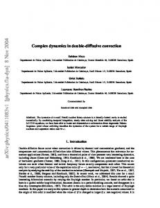
Figure 3: Dynamical response of model system (12) with predation rate ℎ1 = 0.07.

0.8 14 Zooplankton

0.78 0.76

Nutrient

0.74 0.72 0.7

13.9 13.85 13.8 0.24

0.68

Phy

0.66 0.64 0.62

0.22 top 0.2 lan kto n

0.18

0.71 0.7 0.69 t n e 0.68 i Nutr 0.67

0.72

0.0745

0.074

0.0735

0.073

0.0725

0.072

0.0715

0.071

Figure 4: Phase portrait of model system (12) with predation rate ℎ1 = 0.07. 0.0705

0.07

13.95

h1

Figure 2: Bifurcation diagram of Poincaré section for the nutrient and predation rate ℎ1 is varied in [0.07, 0.075].

and the above computation that model system (12) undergoes transcritical bifurcation around 𝑀∗ . 4.2. Numerical Experiments for Model System without Seasonality. In order to facilitate the following numerical experiments, some preliminaries about Poincaré surface-ofsection technique and Lyapunov exponents are introduced in Remarks 6 and 7. Remark 6. A traditional approach to gain preliminary insight into the properties of dynamical system is to carry out a onedimensional bifurcation analysis. One-dimensional bifurcation diagrams of Poincaré maps present information about

the dependence of the dynamics on a certain parameter. The analysis is expected to reveal the type of attractor to which the dynamics will ultimately settle down after passing the initial transient phase and within which the trajectory will then remain forever. On a Poincaré surface of section, the dynamical behavior can be described by a discrete map whose phase-space dimension is less than that of the original continuous flow. Chaotic flows can be understood based on concepts that are convenient for maps such as unstable orbits (see [26–28] and references therein). Case 1. A finite number of points corresponds to a periodic solution; that is, one point corresponds to a solution of period equal to that of the forcing term, namely, 2𝜋/𝜔 (periodone); and 𝑛 points correspond to a solution (subharmonic) of period 2𝑛𝜋/𝜔 (period 𝑛 or a subharmonic of order 1/𝑛). Case 2. A closed curve corresponds to a quasiperiodic solution, that is, a solution consisting of two incommensurate

8


3000

3500

4000

4500

0.22 0.2 0.18 0.16 2500

3000

3500

4000

4500

5000

Time

13.8 13.6 13.4 2500

3000

3500

4000

4500

5000


Zooplankton

0

0.5

1000

2000

3000

4000

5000

3000

4000

5000

3000

4000

5000

Time 0.4 0.2 0

0

1000

2000 Time

12 10 8 0

1000

2000 Time

Time

12 11.8 11.6 11.4 11.2 11 10.8 10.6 10.4 0.4 0.35 0.3 0.25 Phy 0.2 top 0.15 lank 0.1 ton 0.05

0.8 0.6 0.4 0.2

5000

Time

Phytoplankton

Phytoplankton

0.65 2500

Zooplankton

Nutrient

0.7

Zooplankton

Nutrient

0.75

0.6

0.7

0.8

0.9

1

ient Nutr

Figure 6: A limit cycle corresponding to periodic solution in Figure 5.

frequencies or, equivalently, having a trajectory that is dense on tours. Case 3. A collection of points that is fractal corresponds to chaos, namely, a stranger in phase space; a collection of points that form a cloud that is disorganized, partially organized, or fuzzy may (or may not ) correspond to chaotic attractors. Remark 7. In a given embedding dimension, the Lyapunov exponent is a measure of the speeds at which initially nearby trajectories of the system diverge. There is a Lyapunov exponent for each dimension of the process, which together constitutes the Lyapunov spectrum for the dynamical system. The Lyapunov exponent is related to the predictability of the system, and the largest Lyapunov exponent of a stable system does not exceed zero. However, a chaotic system has at least one positive Lyapunov exponent. A bounded system with a positive Lyapunov exponent is one operational definition of chaotic behaviors, which presents a quantitative measure of the average rate of separation of nearby trajectories on the attractor. Over the years, a number of methods have been introduced for computation of Lyapunov exponents


(see [26, 28]). A positive Lyapunov exponent implies that a chaotic process displays long term unpredictability, with the output being sensitively dependent on the initial conditions. Even slightly different initial values can lead to vastly different system outputs. Furthermore, another characteristic for chaos is fractal dimension, which can be computed with the commutated Lyapunov exponents (see Section 9.4 of reference [29]). In the absence of seasonality, we will perform numerical experiments to observe the dynamics of the model system (2) with the following hypothetical set of parameter values, which are given as follows: 𝑟0 = 1, 𝐾 = 1, 𝑎 = 1.63, 𝑟1 = 0.01, 𝑟2 = 0.001, 𝑐1 = 0.95, 𝑏1 = 0.33, 𝑑1 = 0.4, 𝑐2 = 0.9, 𝑑2 = 0.01, 𝑏2 = 0.5, 𝑞 = 0.1, and 𝐸 = 0.15. In the following part, ℎ1 (predation rate) is chosen as bifurcation parameter. By virtue of scaling introduced in model system (12), values of parameters are obtained as follows: 𝛼 = 4.94, 𝛽1 = 3.03, 𝑚1 = 4.69, 𝑓1 = 0.01, 𝑓2 = 0.001, 𝑚2 = 0.9ℎ1 , 𝜖1 = 0.4, 𝜖2 = 0.01, 𝛽2 = 2, and 𝐸1 = 0.015. A bifurcation diagram of Poincaré section is plotted to investigate the dynamic effect of predation rate on model system (12), which can be shown in Figure 1. In order to understand Hopf bifurcation occurring at the critical value ℎ1∗ = 0.0711, bifurcation diagram with (0.07, 0.075) is plotted in Figure 2. According to (15) and (16), it can be obtained that ℎ1 > 0.068 guarantees the existence of interior equilibrium. Based on Figures 1 and 2, it is observed that model system (12) is stable around the interior equilibrium when ℎ1 varies within (0.068, 0.0711). It should be noted that ℎ1 = 0.07 is randomly selected within (0.068, 0.0711); the dynamical response and phase portrait of model system (12) with ℎ1 = 0.07 is plotted in Figures 3 and 4, respectively, which shows that model system (12) is locally asymptotically stable around interior equilibrium 𝑀∗ (0.7022, 0.1999, 13.9114).


9

Zooplankton

12 11 10 9 8 0.8

0.6 Ph yto 0.4 pla nkt on

0.2

0

0.2

0.4

0.6 t r ien Nut

0.8

1

Figure 8: Phase portrait of model system (12) with predation rate ℎ1 = 0.08. Table 1: Lyapunove exponents and corresponding Lyapunov dimensions of model system (12) with ℎ1 = 0.08, 0.085, 0.09, 0.095, and 0.1.

𝐿1 𝐿2 𝐿3 𝐷

0.08 0.13761 0 −1.1265 2.1222

0.085 0.1543 0 −1.5804 2.0976

ℎ1 0.09 0.1818 0 −1.5803 2.115

0.095 0.1913 0 −1.5893 2.1204

0.1 0.2044 0 −1.5710 2.1301

As ℎ1 increases across the critical value ℎ1∗ = 0.0711; model system enters into Hopf bifurcation. Dynamical responses of model system (12) with ℎ1∗ = 0.0711 is plotted in Figure 5, and a limit cycle corresponding to periodic solution is observed in Figure 6. As ℎ1 further increases, it leads to a chaotic region at ℎ1 ∈ (0.0711, 0.1). The dynamical response and phase portrait of model system with ℎ1 = 0.08 is plotted in Figures 7 and 8, respectively. It should be noted that the sensitive dependence of future dynamics on the current state, the signature of chaotic behavior, is apparent from the fact that all the trajectories in the handle of teacup are very close together. Based on Theorem 4, model system undergoes Hopf bifurcation at critical bifurcation value ℎ1∗ = 0.0711. With the increase of bifurcation parameter ℎ1 , it can observed that model system enters into period doubling from limit cycle oscillations based on Figure 2, and model system finally settles down into chaotic behavior from period doubling. Hence, it can be concluded that model system admits that the transition to chaos is realized through the cascade of period doubling bifurcations. Furthermore, chaotic attractor of model system (12) with ℎ1 = 0.085, 0.09, 0.095, and 0.1 are plotted in Figure 9, and the corresponding Poincaré section of Figure 9 is plotted in Figure 10, which coincides with Case 3 introduced in Remark 6 implying the occurrence of chaotic attractor. Lyapunov exponents (denoted by 𝐿 𝑖 , 𝑖 = 1, 2, 3) with time and the corresponding Lyapunov dimensions can be computed, which are utilized to show the existence of chaotic attractor. Table 1 shows Lyapunov exponents and corresponding Lyapunov dimensions of model system (12) with ℎ1 = 0.08, 0.085, 0.09, 0.095 and 0.1.

It follows from the Table 1 that there is a positive Lyapunov exponent for the model system (12) with ℎ1 = 0.08, 0.085, 0.09, 0.095, and 0.1, respectively. Furthermore, it follows from the Table 1 that Lyapunov dimensions for model system (12) with ℎ1 = 0.08, 0.085, 0.09, 0.095, and 0.1 are all fractals. According to the characterization of chaotic attractors introduced in Remark 7, a bounded system with a positive Lyapunov exponent is one operational definition of chaotic behavior, and another characteristic for chaos is fractal dimension. Oscillatory population may be driven to extinction in presence of environmental stochasticity when the population density is very low [30]. Based on the above numerical experiments, chaotic dynamics for increasing the predation rate has been discussed. In the following part, role of harvesting in controlling chaotic dynamics will be investigated. Now we fixed the predation rate ℎ1 = 0.08 in chaotic region and the harvest effort 𝐸1 is chosen as bifurcation parameter. Figure 11 shows the bifurcation diagram of Poincaré section for the nutrient and harvest effort 𝐸1 is varied in [0, 0.15]. It should be noted that harvest effort 𝐸1 should be controlled within [0, 0.15] based on (15) and (16), which guarantees the existence of interior equilibrium. From Figure 11, it is observed that chaotic behavior remains for 𝐸1 that varies from [0, 0.1381). With the increase of 𝐸1 , chaos enter into limit cycle oscillation at 𝐸1 = 0.1381 and finally the model system (12) enters into stable focus from limit cycle. 4.3. Numerical Experiments for Model System with Seasonality. With the help of MATLAB, numerical experiments with hypothetical set of parameters are performed to understand the dynamical effect of seasonal intrinsic growth rate of nutrient biomass on model system (2). The values of parameters are given as follows: 𝑟0 = 1, 𝐾 = 1, 𝑎 = 1.63, 𝑟1 = 0.01, 𝑟2 = 0.001, 𝑐1 = 0.95, 𝑏1 = 0.33, 𝑑1 = 0.4, 𝑐2 = 0.9, 𝑑2 = 0.01, 𝑏2 = 0.5, ℎ = 0.04, 𝑞 = 0.1, 𝐸 = 0.15, and 𝜔 = 2. By choosing Γ as a bifurcation parameter, bifurcation diagram of Poincaré section for the nutrient and Γ is varied in [0, 1], which can be found in Figure 12. It can be observed that chaotic behavior enters into periodic attractor when bifurcation parameter Γ increases through a critical value Γ = 0.8. Model system (2) admits periodic attractor Γ within the range [0.8, 1]. It should be noted that Γ = 0.81 and Γ = 0.95 are randomly selected from [0.8, 1]. Dynamical responses of model system with Γ = 0.81 and Γ = 0.95 are plotted in Figures 13 and 14, respectively. Corresponding Poincaré section of model system (2) with Γ = 0.81 is plotted in Figure 15(a), which coincides with Case 1 introduced in Remark 6 implying the existence of periodic attractor; and corresponding Poincaré section of model system (2) with Γ = 0.95 is plotted in Figure 15(b), which coincides with Case I introduced in Remark 6 implying the existence of periodic attractor. Poincaré points 5000–15000 are plotted. Based on the above numerical experiments, chaotic behavior can be controlled by the enhancement of amplitude of seasonal intrinsic growth of nutrient biomass; such type of mechanism reduces chaotic behavior to periodic attractor.

10


12

12

z(t)

z(t)

h1 = 0.09

h1 = 0.085

14

10 0.4 p(t

)

8 0.5

1

0.2 0

0

10

p(t

0.5 ) n (t

1 )

0

(a)

z(t)

z(t)

8 0.5

1 t)

0

0

)

h1 = 0.1

15

10

p(

n (t

(b)

h1 = 0.095

12

0

0.5

0.5 ) x(t

10

5 0.5

1

p(t

)

(c)

0

0

0.5 ) n (t

(d)

Figure 9: Chaotic attractor of model system (12) with predation rate ℎ1 = 0.085, 0.09, 0.095, 0.1.

Remark 8. It can be observed that the dynamical responses fluctuate with complex structures when the model system admits chaotic behavior. Especially, some dynamical response even comes close to zero within some time interval, which biologically reflects harmful phytoplankton bloom. Consequently, there has been considerable scientific attention towards harmful phytoplankton bloom and its associate control strategy. Based on the theoretical analysis, it is found that high nutrient levels and favorable conditions play a key role in rapid or massive growth of phytoplankton bloom; low nutrient concentration, high predation pressure from zooplankton, and other unfavorable conditions limit phytoplankton growth, which leads to oscillations or recurring bloom in the nutrient-phytoplankton-zooplankton marine ecosystem. Based on the numerical experiments shown in Figure 11, harvesting has a stabilizing effect on model dynamics. Furthermore, numerical experiments show that chaotic behavior of the population due to enhancement of predation rate can be prevented by adopting a suitable harvesting policy and model system (12) eventually approaches to a stable steady state. If the harvest effort on phytoplankton population increases, the zooplankton population decreases due to lack of the phytoplankton population and nutrient absorption pressure decreases and in turn the nutrient within marine system increases. On the other hand, harvest effort should be constrained within certain interval, which may guarantee the existence of nutrient biomass, phytoplankton population, and

zooplankton population within marine system. The theoretical findings obtained in the above section are of inspiration for regulating some constructive policies to control harmful phytoplankton bloom with the introduction of appropriate harvest effort.

5. Conclusion It is well known that phytoplankton population and zooplankton population play a key role in large-scale global processes such as ocean-atmosphere dynamics and climate change. Plankton population constitutes the bottom level of the marine and terrestrial life. Recently, harmful algal blooms (HAB) are widely reported and have become a serious environmental problem worldwide as its serious social and economic consequence. Therefore, a better understanding of mechanisms that determine the plankton dynamics is of considerable interest in recent decades [4–13]. Considering the economic interest of exploitation of phytoplankton and seasonal variation of nutrient biomass, a dynamical model is proposed in this paper. It is utilized to discuss the interaction mechanism of nutrient-phytoplankton-zooplankton marine system, where harvest effort on phytoplankton population is considered as well as seasonal intrinsic rate of nutrient biomass. Conditions for positivity and boundedness of solutions are obtained in Theorems 1 and 2, respectively. By choosing predation rate as bifurcation parameter, local stability analysis of model system (12) is performed around the interior equilibrium and sufficient conditions for occurrence


11

h1 = 0.085

0.4

0.3

p(t)

p(t)

0.3

0.2

0.1

0 0.2

h1 = 0.09

0.4

0.2

0.1

0.4

0.6

0.8

0 0.2

1

n(t) (a)

1

0.3

p(t)

p(t)

0.8

h1 = 0.1

0.4

0.3

0.2

0.2

0.1

0.1

0 0.2

0.6 n(t) (b)

h1 = 0.095

0.4

0.4

0.4

0.6

0.8

1

0

0

0.5 n(t)

n(t) (c)

1

(d)

Figure 10: Corresponding Poincaré section of model system (12) with ℎ1 = 0.085, 0.09, 0.095, 0.1. Poincaré points 5000–15000 are plotted.

1.1 1 0.9 Nutrient

0.8 0.7 0.6 0.5 0.4 0.3 0.2 0.1

0

0.05

0.1

0.15

E1

Figure 11: Bifurcation diagram of Poincaré section for the nutrient and harvest effort 𝐸1 is varied in [0, 0.15].

of Hopf bifurcation are obtained, which can be found in Theorems 3 and 4, respectively. Further attempts are made to understand the effect of harvest effort and seasonality on population dynamics of the model system. Numerical experiments reveal that harvest effort on phytoplankton population has a stabilizing effect on population dynamics, and the increase of seasonal intrinsic growth of nutrient biomass is responsible for controlling chaotic behavior. Compared with the previous related work [4–6, 8], interaction mechanism of phytoplankton and zooplankton is discussed in this paper, and the effect of predation from zooplankton and nutrient recycling within nutrientphytoplankton-zooplankton ecosystem are also studied. Compared with the previous related work [14–17, 21], nutrient recycling within marine ecosystem and seasonality of nutrient biomass are considered and investigated in this paper. Furthermore, the stabilizing effect on model system that concentrates on control strategies for chaotic behavior is also discussed. Generally, nutrient-phytoplankton-zooplankton

12


Nutrient

1.4

0.5

1.2 1

Phytoplankton

N(t)

0.8 0.6 0.4

Nutrient

4900 Time

4850

4900

4950

5000

0.16 0.15 4800

4950

5000

Time

0.1

0.2

0.3

0.4

0.5 Γ

0.6

0.7

0.8

0.9

1

Zooplankton

0

2

12 10 8 0

1000

2000

Time

3000

4000

5000

Figure 14: Dynamical response of model system (2) with Γ = 0.95.

1 0 4800

Γ = 0.81 4850

4900 Time

4950

5000

4850

4900 Time

4950

5000

P (t)

0.12 0.1 0.08 4800

0.25 0.2 0.15 0.1 0.05 0

0

0.1

0.2

0.3

0.5

0.6

0.7

0.8

0.5

0.6

0.7

0.8

Γ = 0.95

10 5 0

0.4 N (t) (a)

15

0

1000

2000

3000

4000

5000

Time

Figure 13: Dynamical response of model system (2) with Γ = 0.81.

P (t)

Phytoplankton

4850

0.17

Figure 12: Bifurcation diagram of Poincaré section for the nutrient and Γ is varied in [0, 1].

Zooplankton

0 4800

0.18

0.2 0

1

0.25 0.2 0.15 0.1 0.05 0

0

0.1

0.2

0.3

0.4 N (t) (b)

ecosystem is often deeply perturbed by human exploiting activities; some biological interpretations about the theoretical analysis obtained in this paper are also provided that can be found in Remark 8, which are beneficial to discussing interaction and coexistence mechanism of population within the harvested marine ecosystem. It makes the work studied in this paper have some new and positive features.

Figure 15: Corresponding Poincaré section of model system (2) with Γ = 0.81 is plotted in (a), and corresponding Poincaré section of model system (2) with Γ = 0.95 is plotted in (b). Poincaré points 5000–15000 are plotted.

Acknowledgments Conflict of Interests All authors of this paper declare that there is no conflict of interests regarding the publication of this paper. The authors have no proprietary, financial, professional, or other personal interest of any nature or kind in any product, service, and/or company that could be construed as influencing the position presented in, or the review of, this paper.

The authors gratefully acknowledge anonymous reviewers, editors and Professor Lev Ryashko’s comments. This work is supported by National Natural Science Foundation of China, Grant no. 61104003, Grant no. 61273008, and Grant no. 61104093; Research Foundation for Doctoral Program of Higher Education of Education Ministry, Grant no. 20110042120016; Hebei Province Natural Science Foundation, Grant no. F2011501023; Fundamental Research Funds for the

Mathematical Problems in Engineering Central Universities, Grant no. N120423009; Research Foundation for Science and Technology Pillar Program of Northeastern University at Qinhuangdao, Grant no. XNK201301. This work is supported by State Key Laboratory of Integrated Automation of Process Industry, Northeastern University, supported by Hong Kong Admission Scheme for Mainland Talents and Professionals, Hong Kong, Special Administrative Region.

References [1] C. M. Lalli and T. R. Parsons, Biological Oceanography: An Introduction, Butterworth-Heinemann, Oxford, UK, 1997. [2] M. N. Antonios, “A mathematical model of two-trophic-level aquatic systems with two complementary nutrients,” Mathematical Biosciences, vol. 84, no. 2, pp. 231–248, 1987. [3] M. Kot, Elements of Mathematical Biology, Cambridge University Press, Cambridge, UK, 2001. [4] J. Chattopadhyay, R. R. Sarkar, and S. Pal, “Dynamics of nutrient-phytoplankton interaction in the presence of viral infection,” BioSystems, vol. 68, no. 1, pp. 5–17, 2003. [5] D. T. Dimitrov and H. V. Kojouharov, “Analysis and numerical simulation of phytoplankton-nutrient systems with nutrient loss,” Mathematics and Computers in Simulation, vol. 70, no. 1, pp. 33–43, 2005. [6] B. Mukhopadhyay and R. Bhattacharyya, “Modelling phytoplankton allelopathy in a nutrient-plankton model with spatial heterogeneity,” Ecological Modelling, vol. 198, no. 1-2, pp. 163– 173, 2006. [7] S. R. J. Jang, J. Baglama, and J. Rick, “Nutrient-phytoplanktonzooplankton models with a toxin,” Mathematical and Computer Modelling, vol. 43, no. 1-2, pp. 105–118, 2006. [8] S. Pal, S. Chatterjee, and J. Chattopadhyay, “Role of toxin and nutrient for the occurrence and termination of plankton bloom—results drawn from field observations and a mathematical model,” BioSystems, vol. 90, no. 1, pp. 87–100, 2007. [9] S. Khare, O. P. Misra, and J. Dhar, “Role of toxin producing phytoplankton on a plankton ecosystem,” Nonlinear Analysis: Hybrid Systems, vol. 4, no. 3, pp. 496–502, 2010. [10] N. H. Gazi and K. Das, “Structural stability analysis of an algal bloom mathematical model in tropic interaction,” Nonlinear Analysis: Real World Applications, vol. 11, no. 4, pp. 2191–2206, 2010. [11] T. Zhang and W. Wang, “Hopf bifurcation and bistability of a nutrient-phytoplankton-zooplankton model,” Applied Mathematical Modelling, vol. 36, no. 12, pp. 6225–6235, 2012. [12] Q. H. Cai, Z. Mohamad, and Y. Yuan, “Modelling on an ecological food chain with recycling,” Communication Nonlinear Science and Numerical Simulation, vol. 17, pp. 4856–4859, 2012. [13] A. J. Fan, P. Han, and K. F. Wang, “Global dynamics of a nutrient-plankton system in the water ecosystem,” Applied Mathematics and Computation, vol. 219, pp. 8269–8276, 2013. [14] S. Gakkhar and R. K. Naji, “Seasonally perturbed prey-predator system with predator-dependent functional response,” Chaos, Solitons and Fractals, vol. 18, no. 5, pp. 1075–1083, 2003. [15] S. M. Moghadas and M. E. Alexander, “Dynamics of a generalized Gause-type predator-prey model with a seasonal functional response,” Chaos, Solitons and Fractals, vol. 23, no. 1, pp. 55–65, 2005.

13 [16] S. Gakkhar, K. Negi, and S. K. Sahani, “Effects of seasonal growth on ratio dependent delayed prey predator system,” Communications in Nonlinear Science and Numerical Simulation, vol. 14, no. 3, pp. 850–862, 2009. [17] M. Gao, H. Shi, and Z. Li, “Chaos in a seasonally and periodically forced phytoplankton-zooplankton system,” Nonlinear Analysis: Real World Applications, vol. 10, no. 3, pp. 1643–1650, 2009. [18] C. W. Clark, Mathematical Bioeconomics: The Optimal Management of Renewable Resource, John Wiley and Sons, New York, NY, USA, 2nd edition, 1990. [19] T. K. Kar and U. K. Pahari, “Modelling and analysis of a preypredator system with stage-structure and harvesting,” Nonlinear Analysis: Real World Applications, vol. 8, no. 2, pp. 601–609, 2007. [20] T. K. Kar and A. Ghorai, “Dynamic behaviour of a delayed predator-prey model with harvesting,” Applied Mathematics and Computation, vol. 217, no. 22, pp. 9085–9104, 2011. [21] Y. Lv, Y. Pei, S. Gao, and C. Li, “Harvesting of a phytoplanktonzooplankton model,” Nonlinear Analysis: Real World Applications, vol. 11, no. 5, pp. 3608–3619, 2010. [22] H. R. Thieme, Mathematics in Population Biology, Princeton University Press, Princeton, NJ, USA, 2003. [23] H. I. Freedman and R. M. Mathsen, “Persistence in predatorprey systems with ratio-dependent predator influence,” Bulletin of Mathematical Biology, vol. 55, no. 4, pp. 817–827, 1993. [24] W. M. Liu, “Criterion of hopf bifurcations without using eigenvalues,” Journal of Mathematical Analysis and Applications, vol. 182, no. 1, pp. 250–256, 1994. [25] J. Guckenheimer and P. Holmes, Nonlinear Oscillations, Dynamical Systems, and Bifurcations of Vector Field, Springer, New York, NY, USA, 1983. [26] F. Takens, Detecting Strange Attractor in Turbulence, Dynamical Systems and Turbulence, Lecture Notes in Mathematics, Springer, New York, NY, USA, 1981. [27] A. Wolf, J. B. Swift, H. I. Swinney, and J. A. Vastano, “Determining Lyapunov exponents from a time series,” Physica D: Nonlinear Phenomena, vol. 16, no. 3, pp. 285–317, 1985. [28] T. S. Parker and L. O. Chua, Practical Numerical Algorithms for Chaotic Systems, Springer, New York, NY, USA, 1989. [29] J. Kaplan and J. Yorke, “Chaotic behavior of multidimensional difference equations,” in Functional Differential Equations and Approximation of Fixed Points, Lecture Notes in Mathematics, Springer, Berlin, Germany, 1979. [30] A. Fenton and S. A. Rands, “The impact of parasite manipulation and predator foraging behavior on predator-prey communities,” Ecology, vol. 87, no. 11, pp. 2832–2841, 2006.

Advances in

Operations Research Hindawi Publishing Corporation http://www.hindawi.com

Volume 2014

Advances in

Decision Sciences Hindawi Publishing Corporation http://www.hindawi.com

Volume 2014

Journal of

Applied Mathematics

Algebra

Hindawi Publishing Corporation http://www.hindawi.com


Volume 2014

Journal of

Probability and Statistics Volume 2014

The Scientific World Journal Hindawi Publishing Corporation http://www.hindawi.com


Volume 2014

International Journal of

Differential Equations Hindawi Publishing Corporation http://www.hindawi.com

Volume 2014

Volume 2014

Submit your manuscripts at http://www.hindawi.com International Journal of

Advances in

Combinatorics Hindawi Publishing Corporation http://www.hindawi.com

Mathematical Physics Hindawi Publishing Corporation http://www.hindawi.com

Volume 2014

Journal of

Complex Analysis Hindawi Publishing Corporation http://www.hindawi.com

Volume 2014

International Journal of Mathematics and Mathematical Sciences


Journal of

Mathematics Hindawi Publishing Corporation http://www.hindawi.com

Volume 2014


Volume 2014

Volume 2014


Volume 2014

Discrete Mathematics

Journal of

Volume 2014


Discrete Dynamics in Nature and Society

Journal of

Function Spaces Hindawi Publishing Corporation http://www.hindawi.com

Abstract and Applied Analysis

Volume 2014


Volume 2014


Volume 2014

International Journal of

Journal of

Stochastic Analysis

Optimization



Volume 2014

Volume 2014